Uncertainty Quantification in Hybrid Dynamical Systems
Abstract
Uncertainty quantification (UQ) techniques are frequently used to ascertain output variability in systems with parametric uncertainty. Traditional algorithms for UQ are either system-agnostic and slow (such as Monte Carlo) or fast with stringent assumptions on smoothness (such as polynomial chaos and Quasi-Monte Carlo). In this work, we develop a fast UQ approach for hybrid dynamical systems by extending the polynomial chaos methodology to these systems. To capture discontinuities, we use a wavelet-based Wiener-Haar expansion. We develop a boundary layer approach to propagate uncertainty through separable reset conditions. We also introduce a transport theory based approach for propagating uncertainty through hybrid dynamical systems. Here the expansion yields a set of hyperbolic equations that are solved by integrating along characteristics. The solution of the partial differential equation along the characteristics allows one to quantify uncertainty in hybrid or switching dynamical systems. The above methods are demonstrated on example problems.
1 Introduction
Uncertainty Quantification (UQ) is an area of mathematics that is used to quantify output distributions given parametric uncertainty. Traditional approaches include Monte Carlo and Quasi-Monte Carlo methods [1], response surface methods [2, 3] as well as polynomial chaos and probabilistic collocation based approaches [4]. The polynomial chaos approach for uncertainty quantification was originally proposed by Norbert Wiener [5]. Assuming that one is given input uncertainty in the form of distributions associated with various parameters of the system, polynomial chaos/probabilistic collocation methods provide an approach for fast uncertainty quantification under the assumption of smooth dynamics. In particular, polynomial chaos provides exponential convergence for smooth systems and processes with finite variance [4]. Polynomial chaos based methods have been used for a multitude of applications, see [6, 7, 8, 9, 10, 11, 12, 13] for examples. Note that, depending on the application, one can combine various UQ approaches. For example, a combination of polynomial chaos and the response surface methodology has been used to develop probabilistic collocation methods for discrete distributions in [10].
In this work, we focus on developing UQ techniques for hybrid dynamical systems. Hybrid dynamical systems theory is used to model systems with both discrete and continuous dynamics [14]. Examples include the bouncing ball automaton [15], biological networks [16, 17], air traffic management systems [18], communication networks [19], elevators, and robotics, to name a few. These systems frequently display rich dynamics not seen in continuous systems. For example, Zeno behavior in hybrid systems is characterized by an infinite number of discrete switches in finite time [15, 20]. Hybrid systems can be particularly challenging from an analysis standpoint since traditional techniques, such as polynomial chaos based methods, assume smoothness, rendering them inapplicable.
In this work, we develop polynomial chaos and transport theory based methods for propagating uncertainty through hybrid systems. We assume that the domains associated with different modes of operation of the hybrid system do not overlap. We demonstrate that, by integrating over appropriate time-varying regions, one can extend the polynomial chaos framework to hybrid dynamical systems. We resolve the issue of state resets [14] in the separable case by using boundary layer approximations. To capture the discontinuities in the probability distributions of the output variables, we use a Haar-wavelet expansion [21]. This expansion has previously been used in the polynomial chaos setting to propagate uncertainty through dynamical systems close to bifurcation points [9, 22, 23]. Here we develop a methodology to propagate uncertainty through systems with discontinuities in dynamics and output along with state resets. We also develop a transport theory based approach that allows one to propagate the uncertainties through the various modes of the hybrid dynamical system.
Our paper is organized as follows: in section 2 we define hybrid dynamical systems and the problem of uncertainty quantification. In section 3 we first construct the framework for polynomial chaos in the hybrid dynamical system setting (3.1). We then demonstrate the Haar wavelet expansion for hybrid polynomial chaos in 3.2. The handling of state resets is considered in section 3.3. Finally, the results on hybrid polynomial chaos are presented in 3.4. The transport operator theory based method for propagating uncertainty through hybrid dynamical systems is developed in section 4 and conclusions are drawn in section 5.
2 Problem definition
Let denote a hybrid system , where
Set of discrete variables Set of continuous variables Vector field Set of initial conditions Domain Set of discrete transitions Guard conditions Reset map.
In the above table, is the tangent bundle of and is the power set of . For more details on the definition of hybrid systems, see [14].
We can use the following representation for hybrid systems,
| (1) |
where is a vector of state variables and the form of is dictated by , which represents the mode of operation of the hybrid dynamical system. The discrete state is determined by the guard conditions that dictate transitions between modes (see Fig. 1). The reset functions are a part of the reset map . In Eqn. 1 let denote the vector of system parameters and the initial condition for the system.

If the system parameters in Eqn. 1 are uncertain (i.e., each has an associated distribution) then one typically desires to quantify the time-varying moments (such as mean and variance) of (note that may also be uncertain). As mentioned earlier, although one can use Monte Carlo based sampling methods [1], they are plagued by slow convergence. In particular, the mean is expected to converge as , where is the number of samples. Quasi-Monte Carlo based sampling methods are expected to give a convergence rate of , where is the dimensionality of the random space [24], making these methods attractive for problems in low dimensions. Polynomial chaos based methods provide an alternative framework for uncertainty quantification with exponential convergence for processes with finite variance, but they too suffer from the curse of dimensionality [4]. In the next section we extend the polynomial chaos framework to hybrid systems.
3 Polynomial chaos for hybrid dynamical systems
Starting with a complete probability space given by , where is the sample space, is the -algebra on and is a probability measure, let denote the Hilbert space of square-integrable, -measurable, -valued random elements. Then one can, in general, define a polynomial chaos basis , where is a random vector and is a vector of non-negative indices. We denote the probability density function of the random vector by .
Generalized polynomial chaos (gPC) [25], provides a framework for representing second-order stochastic processes for arbitrary distributions of by the following expansion:
| (2) |
where is the sum of the indices of and are orthogonal polynomials on with respect to , i.e.
| (3) |
where is the Kronecker delta product. Depending on one can generate an appropriate orthogonal basis for representing . For example, if is Gaussian, then the appropriate polynomial chaos basis is the set of Hermite polynomials; if is the uniform distribution, then the basis is the set of Legendre polynomials. For details on the correspondence between distributions and polynomials see [4, 26]. A framework to generate polynomials for arbitrary distributions has been developed in [25].
In practice, the expansion in Eqn. 2 is truncated at a particular order, say, . One can then use Galerkin projections to obtain a set of differential equations for the coefficients in Eqn. 2 [4].
We now extend the standard polynomial chaos framework to hybrid dynamical systems despite the presence of switching and state resets. To the best of our knowledge, it is the first attempt to develop tools for fast uncertainty quantification for this class of systems.
3.1 Hybrid Polynomial Chaos
Without loss of generality, consider the following two-mode hybrid dynamical system as representative of systems in which the different operating modes are associated with non-overlapping regions:
| (4) |
Here one desires to quantify , i.e., determine as a function of time and parameters . The system above has two modes of operation determined by its state. One can parameterize these modes in the following way:
| (5) | |||||
| (6) |
When (corresponding to ) the governing differential equations are , and when () the governing differential equations are . Thus, one can rewrite Eqn. 4 as,
| (7) |
This equation extends easily to modes of operation by constructing indicator functions for each mode of operation of the hybrid system. We now expand in the appropriate orthogonal polynomial chaos basis,
| (8) |
Dropping the arguments of and for simplicity and using the above relation with Eqn. 7, one gets
By multiplying the above relation by , integrating over , and using orthogonality conditions, we get
| (9) | |||||
Note that and . Thus by evaluating the two integrals one can evolve for any index vector . Note, however, that the regions of integration and are time-dependent quantities and must be evaluated at every instant in time. For a pictorial depiction of and , see Fig. 2.

3.2 Hybrid Polynomial Chaos and wavelet expansions
Hybrid systems can display discontinuous behavior as a function of the uncertain parameters. In view of this, a smooth polynomial chaos expansion is expected to degrade as the discontinuities become more severe. In Ref. [22] the authors develop a wavelet-based Wiener-Haar expansion to treat bifurcating (but smooth) dynamical systems with uncertain initial conditions that result in discontinuous behavior. In this section we adapt the Wiener-Haar expansion to hybrid dynamical systems.
In [22, 23], output variables are expanded in terms of Wiener-Haar wavelets expressed as functions of the Cumulative Distribution Function (CDF) of the uncertain parameters. For simplicity, consider the univariate case. Here we denote the CDF of the uncertain parameter as and expand the state vector as11 1 For the multivariate case, see Ref. [22].
| (10) |
where,
is a family of Haar wavelets [21], defined in terms of the mother wavelet:
The index determines the scale of the wavelet and its displacement. Note that is a family of orthonormal functions on the interval with respect to the uniform density. This makes the family automatically orthonormal with respect to the probability density of :
Additionally, all ’s are orthogonal to the constant function on , which implies that the mean of is given by the first term in the expansion
and that the variance is
We now use this expansion on a switching oscillator example:
| (11) |
which can be rewritten as,
The expansion in this case is
Projecting these equations onto the basis functions yields,
Note that to compute we invert the CDF .
To compute the integrals needed to evolve these equations numerically, we take advantage of the fact that Haar wavelets are piecewise constant. Namely, for a given truncation order , if we divide into equal subintervals, both (with ) and the truncated expansion for (and therefore the indicator functions) are constant in each subinterval. This implies that in each subinterval we only need to calculate the integral of , which is known a priori. For the case of a Gaussian , we have
which has a primitive,
Therefore the contribution to of the integrals in each subinterval is either zero or times the precomputed value
Section 3.4 presents the results obtained with the Wiener-Haar wavelet expansion in Eq. 10 for hybrid dynamical systems.
3.3 Modeling state resets
A significant challenge that hybrid dynamical systems present is the possibility of state resets [14]. When a hybrid system switches from one mode to another, the state of the system can, in general, be reset discontinuously. For example, in the case of the bouncing ball [14], the velocity of the ball changes discontinuously after every impact. When the hybrid system transitions from mode to the state resets are typically represented as,
| (12) |
where and are the states of the system before and after the reset. Such discontinuities cannot be easily accommodated within the hybrid polynomial chaos framework as described in the previous sections.
To circumvent this problem, one can construct a boundary layer in the vicinity of the guard condition. We also introduce a dummy vector () that tracks the state outside the boundary layer and is set to within the boundary layer. Note that we assume separability of the states, i.e. the guard conditions (which determine the switching between modes of operation) can be written independently of the state reset conditions in Eqn. 12. In other words, the states that determine the guard conditions do not participate in the state reset. Let the reset condition be in terms of vector in Eqn. 12, and the guard conditions be in terms of vector (given by ). Note that, represents the entire state vector with the following governing equation,
| (13) |
We now construct a boundary layer around the guard condition for vector as follows:
| (14) |
The above dynamical system is constructed such that evolves to in , where is a small parameter.
By replacing each reset condition with an equation of the form given by Eqn. 14, one obtains a new dynamical system without resets that approximates the original. On this new dynamical system one can use the expansion from Sec. 3.1 and evolve it using Eqn. 9. In other words, the framework generalizing polynomial chaos to hybrid systems can be augmented using Eqn. 14 to include state resets.
To illustrate the procedure presented above we turn to the classic bouncing ball example [15]: we consider the dynamics of a ball bouncing on a floor with coefficient of restitution under the action of gravity of uncertain magnitude ( and ). Thus, every time the ball makes contact with the floor the velocity is reset to a new value given by . The guard condition for resetting the velocity is given by (where is the height of the ball above the floor at time ). The equations for the bouncing ball are given by,
| (15) |
with the reset condition at : . Thus, if one uses the boundary layer approximation in Eqn. 14 we get,
| (16) |
We now use the hybrid polynomial chaos expansion in Eqn. 9 along with the Wiener-Haar wavelet basis functions. The Monte Carlo simulations on the bouncing ball are shown in Fig. 3. The average or nominal trajectory is also shown. In Fig. 3 we compare the nominal trajectory (mean trajectory from Monte Carlo) with the mean predicted using the boundary layer expansion with . As shown, the boundary layer accurately approximates the mean over multiple state resets events (in this case, each impact with the floor).


3.4 Results
To demonstrate the hybrid polynomial chaos approach on hybrid dynamical systems we consider the simple yet challenging example of a switching oscillator given by Eqn. 11.
The value of is deterministic and equal to 0.5. Here we consider three cases with normally distributed with: and (case 1), and (case 2), and and (case 3). In all cases we assume that the initial conditions are deterministic and given by .
3.4.1 Case 1: ,
Let us start with the case when and in Eqn. 11. A representative trajectory for the dynamics of the system is shown in Fig. 4. The corresponding histogram for is shown in Fig. 4. Most importantly, one desires to compute the mean and variance of as a function of time. In the system given by Eqn. 11, we expand using Eqn. 8 and perform a Galerkin projection as shown in Eqn. 9. One then gets a system of equations for the coefficients of expansion in Eqn. 8. These coefficients, once computed, can be used to calculate the moments of the distribution of .
We compare the results obtained from hybrid polynomial chaos with those obtained using Monte Carlo and Quasi-Monte Carlo based methods. In particular, we use a Weyl sequence [27] along with inverse transform sampling [28] to generate the Quasi-Monte Carlo samples. We find that the results (in the first two moments) from samples of Monte Carlo, samples of Quasi-Monte Carlo and the Wiener-Haar hybrid PC expansion with are visually indistinguishable (see Figs. 5 and 5). Treating Monte Carlo samples as baseline, we find that the hybrid PC expansion has a maximum error of in the prediction of .


3.4.2 Case 2: ,
The case of and is significantly more challenging. A representative trajectory of the system (for ) is shown in Fig. 6. When the system switches back and forth between modes. The reason for this is that when the system is in the right half-plane, the equilibrium of the system is in the left half-plane and vice versa. A histogram for is depicted in Fig. 6.
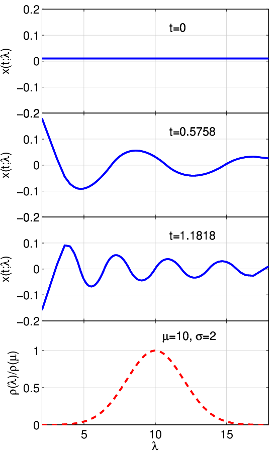
We again compare hybrid Wiener-Haar polynomial chaos to Monte Carlo sampling in Fig. 7. We find that hybrid Wiener-Haar polynomial chaos () accurately computes the mean and the variance of the distribution of . The maximum absolute error of hybrid polynomial chaos in mean is and variance is . Note that expansions in terms of standard basis functions such as Hermite and Legendre polynomials are unable to compute the moments of beyond a threshold time that depends weakly on the order of expansion (see Fig. 8). The solution in this case is particularly challenging because it becomes more oscillatory in terms of at increases (Fig. 9). The Wiener-Haar basis functions are naturally oscillatory and hence more accurate than Hermite polynomials in capturing the solution Note that, for large time simulations the Wiener-Haar expansions will also fail since the solution will eventually become too oscillatory for the order of expansion. This problem is well known in the polynomial chaos literature [29].


3.4.3 Case 3: ,
We also consider the case of with . This case is particularly challenging because there is a concentration of probability of as shown in Fig. 10. The reason for this is as follows: when , the nominal trajectory converges to and so do all trajectories with . Indeed, for trajectories with the equilibrium lies in the opposite half-plane with respect to the current state. This gives rise to decaying switching trajectories, as case 2 in Fig. 6. Note that for , the trajectories are similar to the ones in case 1 (Fig. 4).
The Wiener-Haar basis functions along with the hybrid polynomial chaos approach accurately capture the moments of the distribution for (see Fig. 11). In fact, an expansion to just captures the first two moments. The step-function nature of the Wiener-Haar basis allows it to perform well in this scenario. Standard basis functions like Hermite polynomials are completely incapable of accurately capturing the moments of the distribution for shown in Fig. 6.


4 Transport theory approach for uncertainty quantification in hybrid systems
In this section we present a qualitatively different approach to UQ in hybrid systems based on transport equations. We write an advection equation for the probability density of the state and expand this equation in an appropriate basis, as is done in polynomial chaos. The resulting equation is equivalent to the Fokker-Planck equation [30] in the absence of a diffusion term. Though significant effort has been put into computing solutions for the Fokker-Planck equation in various applications [30, 31], our setting is particularly challenging due to the switching dynamics of hybrid systems. We note that advection equations for probability distribution functions have been used to propagate uncertainty through heterogeneous porous media with uncertain properties [32] and for hyperbolic conservation laws with noise [33]. Recently, similar methods have been extended to cumulative distribution functions in hyperbolic conservation laws [34].
The polynomial chaos expansion in this setting yields a system of hyperbolic partial differential equations for the coefficients of the expansion, which are then solved by integrating along characteristics. The hybrid nature of the original system is reflected in that the characteristics exhibit switching. Even though we only consider systems without resets, we can use the results of Sec. 3.3 to treat systems with resets.
As in Sec. 3, let us consider a hybrid system without resets and uncertain parameters with guard conditions independent of :22 2 Note that this embodies the constraint of having no overlap in the domains for different modes.
The system has uncertain initial conditions described by the probability density and the uncertain parameters follow .
We describe the system by the time evolution of the distribution function , which has initial condition
and normalization
Note that, for all time, we have
| (17) |
Our goal is to compute the evolution of the density in (the marginal distribution):
However, without introducing assumptions on , the equation for is not closed. We therefore focus on computing the evolution of directly through an expansion. From this evolution, can then be calculated at every instant.
4.1 Equation for
Let us define the sets and the indicator functions
With this notation, and because is constant along a trajectory, we have
| (18) |
where and the gradient operator acts only on and not on .
4.2 Boundary conditions at the interfaces
The discontinuity in the equation implies that mass may accumulate at the boundaries between zones where different guard conditions are valid. Integrating on a cylinder that crosses one such boundary we obtain the matching condition
| (19) |
where is a surface probability density between regions and , is the surface normal from to , is the divergence in the space tangent to the surface, and is the flow at the surface.33 3 Whether is or on the surface will depend on how the guard conditions are expressed. This may lead to a cascade, with probability condensing into progressively lower dimensional structures: where two hypersurfaces meet (the boundary between three guard conditions) the same scenario repeats, until we have mass accumulating at points. To solve Eqn. 18 the initial condition must include initial values for and the probability density on any lower dimensional structure where mass may accumulate.
The discontinuity of does not necessarily imply accumulation. In fact, at an interface we have several options:
- 1.
Both and are nonzero and have the same sign. In this case, there is no accumulation. If we assume that has a singularity at the interface, the flow will move the singularity away from it.
- 2.
and : accumulation occurs.
- 3.
and : accumulation occurs.
- 4.
: no accumulation.
- 5.
and : no accumulation.
If we are in the case without accumulation and without initial concentration of density in lower dimensional structures, then and Eqn. 19 becomes
| (20) |
Theorem 1.
Any second order ODE of the form
satisfies the conditions for no accumulation at the interface where the ODE is discontinuous.
Proof.
Without loss of generality we can focus on just two regions and and rewrite the problem as the first-order ODE
To find the normal we consider a function that is positive in and negative so that the interface is given by the locus of . The gradient of this function is proportional to the normal:
and therefore
which is continuous at the interface.
∎
4.3 Expansion of the equation for
At every point we expand the distribution in :
| (21) |
where forms an orthogonal basis with respect to :
We keep to allow for a non-normalized weight function . We replace the expansion in Eqn. 21 into Eqn. 18 and project onto to obtain a set of partial differential equations for the coefficients :
| (22) |
Since this equation is local in there is no question as to which must be used at any given point.
4.4 Example: switching oscillator
Here we revisit the switching oscillator system
which can be expressed as the 2–D system
where and
The transition points are located at and therefore
which is continuous and therefore has the same sign on both sides. Therefore there is no mass accumulation at the interface for this system. This is a special case of theorem 1.
4.4.1 Case 3 revisited
To connect with the example presented in case 3 (, ) we choose and ’s as the probabilist’s Hermite polynomials , with the following properties
Calculating the terms in Eqn. 22:
where the upper sign () is for and the lower sign () is for . Substituting into Eqn. 22 we obtain the equations
| (23) |
Note that, instead of using the Hermite polynomials, one can use the Haar wavelet expansion [22] to represent the solution as was done in previous sections. We plan to present this calculation in future work.
Theorem 2.
The system of PDEs for the switching oscillator is hyperbolic.
Proof.
Consider a system of PDEs of the form
where and the are matrices. The system is hyperbolic if for any the linear combination has real eigenvalues.
For the switching oscillator the system of PDEs can be written as
where . Thus, any combination of the matrices is going to be of the tridiagonal form
This tridiagonal non-symmetric matrix is similar to a tridiagonal symmetric matrix with a diagonal similarity matrix: , where
is similar to , a symmetric and real matrix, and therefore has real eigenvalues.
∎
The issue of hyperbolicity is discussed in more depth in [35]. To solve the hyperbolic system from Eqn. 23 we write it in the form
where is the tridiagonal matrix
| (24) |
We diagonalize and define to obtain the set of uncoupled hyperbolic PDEs
| (25) |
where is the -th eigenvalue. We will now prove that when the expansion is truncated up to , i.e., is truncated to a matrix, the eigenvalues are the zeros of .
Theorem 3.
The eigenvalues of , the truncated version of the matrix in Eqn. 24, are the zeros of the -th order probabilist’s Hermite polynomial .
Proof.
We proceed by induction to prove that , which will then, by the symmetry of , prove our result.
Let . Indeed, and . For the general case,
Therefore,
which is the recurrence relation satisfied by .
∎
The characteristic curves of Eqn. 25 are given by
In other words, the characteristics are damped oscillators where the equilibrium position is given by the eigenvalues of . The exponential growth of along a trajectory is due to the contraction in phase space produced by the dissipation .
4.4.2 Results
We now show results obtained by using transport theory approach on case 3 (, ) for the switching oscillator (Eqn. 11).
In Fig. 12, we show a series of probability distribution snapshots for Monte Carlo ( samples) and the transport operator method (for case 3), gridded in the plane. Note that we set , as defined in the first part of the paper. The Monte Carlo color map snapshots show that the distribution lies on a one-dimensional manifold (in two dimensional space). The one-dimensional nature of the distribution arises because we chose deterministic initial conditions. As discussed previously, all trajectories in case 3 with converge to the origin, resulting in a jump in the cumulative distribution function (CDF).


For , however, the trajectories converge asymptotically to either or . This convergence to or is highly dependent on the individual trajectory and results in a fragmentation of the output distribution. Close to convergence (), very few trajectories converge to a point in the range , as seen in the flat region of the CDF in Fig. 13. The transport-based method captures the singularity at the origin accurately, but is unable to accurately capture the fragmentation. This is because the method samples the distribution sparsely (determined by the order of expansion), resulting in UQ acceleration. However, this sparsity makes the method miss such fine details. On using a high order of expansion (), some samples partially capture the structure around . Note that a much lower order expansion accurately captures the jump at the origin and the asymptotic () shape of the CDF.
As in Fig. 11, we compare Monte Carlo (5000 samples) with the transport theory approach (orders and expansion) in Fig. 14. The (maximum) errors for are (mean) and (variance). For we get errors of and for mean and variance respectively. As shown in Fig. 11, the method performs reasonably well, however, the results are not nearly as good as those obtained using hybrid polynomial chaos with the Wiener-Haar wavelet expansion in section 3.1. However, with a better choice of basis functions, one does expect better results. The transport operator theory is attractive as it appears to be more versatile. In general, the transport operator approach is applicable to hybrid dynamical systems with overlapping modes of operation (by constructing multiple PDEs for the overlapping mode). In contrast, the hybrid polynomial chaos method suffers from the disadvantage of being inapplicable to such systems.


5 Conclusions
As the modeling of hybrid dynamical systems becomes increasingly important for modern day engineering applications such as electrical and biological networks, air traffic systems, communication networks, etc., quantifying uncertainty in these systems is going to become a central concern. Since uncertainty quantification allows one to compute moments of output distributions in the presence of parametric uncertainty, these techniques will be used to aid decisions related to robust system design and performance.
In this work, we have made the first attempts to develop fast uncertainty quantification methods targeted for hybrid dynamical systems. In particular, we extended polynomial chaos methods, a popular technique for propagating uncertainty through smooth systems, to hybrid dynamical systems. We also developed methods to handle state resets within the polynomial chaos framework by using boundary layer approximations. We then applied this new approach to perform uncertainty quantification on switching harmonic oscillators and the bouncing ball examples. We also demonstrated the efficacy of using Wiener-Haar expansions [9, 22, 23] with our hybrid polynomial chaos approach for quantifying uncertainty in hybrid systems that give rise to multi-modal distributions or become increasingly oscillatory in time. Finally, we showed how a transport theory based approach can capture naturally-emerging discontinuities in the distribution. Future efforts involve providing rigorous error bounds for Wiener-Haar expansions in the hybrid polynomial chaos setting with boundary layer expansions. We are also extending our hybrid polynomial chaos approach to networks of hybrid dynamical systems using our recent work on propagating uncertainty through complex networks [36]. We also intend to extend the transport operator based UQ method to hybrid systems with overlapping modes of operation.
6 Acknowledgements
The authors thank Habib Najm for pointing us to his work on Wiener-Haar based polynomial chaos expansion and his insightful input. We also thank Alessandro Pinto and George Mathew for valuable discussions related to hybrid dynamical systems.
References
- [1] R. E. Caflisch. Monte Carlo and quasi-Monte Carlo methods. Acta Numerica, 7:1–49, 1998.
- [2] R. H. Myers, D. C. Montgomery, and C. M. Anderson-Cook. Response Surface Methodology. Wiley, third edition, 2009.
- [3] T. Hastie, R. Tibshirani, and J. Friedman. The Elements of Statistical Learning. Springer, second edition, 2009.
- [4] X. Wan and G. E. Karniadakis. Recent advances in polynomial chaos methods and extensions. In Computational Uncertainty in Military Vehicle Design Meeting Proceedings. NATO/OTAN, Paper Reference Number: RTO-MP-IST-999, 2008.
- [5] N. Wiener. The homogeneous chaos. American Journal of Mathematics, 60(4):897–936, 1938.
- [6] M. S. Allen and J. A. Camberos. Comparison of uncertainty propagation / response surface techniques for two aeroelastic systems,. In 50th AIAA Structures, Structural Dynamics, and Materials Conference, Palm Springs, California, May 4-7, 2009, 2009.
- [7] H. C. Elman, C. W. Miller, E. T. Phipps, and R. S. Tuminaro. Assessment of collocation and Galerkin approaches to linear diffusion equations with random data. Int. J. Uncertainty Quantification, 1:19–23, 2011.
- [8] R. Ghanem. Probabilistic characterization of transport in heterogeneous media. Comput. Methods Appl. Mech. Engng., 158:199–220, 1998.
- [9] H. N. Najm, B. J. Debusschere, Y. M. Marzouk, S. Widmer, and O. P. Le Maître. Uncertainty quantification in chemical systems. Int. J. Numer. Meth. Engng., 80:789–814, 2009.
- [10] T. Sahai, V. Fonoberov, and S. Loire. Uncertainty as a stabilizer of the head-tail ordered phase in carbon-monoxide monolayers on graphite. Physical Review B, 80(11):115413, 2009.
- [11] D. Xiu and G. E. Karniadakis. Modeling uncertainty in flow simulations via generalized polynomial chaos. J. Comp. Phys., 187:137–167, 2003.
- [12] N. Zabaras and B. Ganapathysubramanian. A scalable framework for the solution of stochastic inverse problems using a sparse grid collocation approach. J. Comp. Phys., 227:4697–4735, 2008.
- [13] X. Wan and G. E. Karniadakis. An adaptive multi-element generalized polynomial chaos method for stochastic differential equations. Journal of Computational Physics, 209(2):617–642, 2005.
- [14] C. G. Cassandras and J. Lygeros. Stochastic Hybrid Systems. CRC Taylor & Francis, first edition, 1991.
- [15] K. H. Johansson, M. Egerstedt, J. Lygeros, and S. Sastry. Regularization of Zeno hybrid automata. Systems and Control Letters, 38(3):141–150, 1999.
- [16] R. Alur, C. Belta, F. Ivanic, V. Kumar, M. Mintz, G. Pappas, H. Rubin, J. Schug, and G. J. Pappas. Hybrid Systems: Computation and Control. Springer-Verlag, first edition, 2001.
- [17] N. Chabrier and F. Fages. Symbolic model checking of biochemical networks. In Computational Methods in Systems Biology (CMSB03), volume 2602 of LNCS, pages 149–162. Springer-Verlag, 2003.
- [18] C. Tomlin, G. J. Pappas, and S. Sastry. Conflict resolution for air traffic management: A study in multiagent hybrid systems. IEEE Transactions on Automatic Control, 43:509–521, 1998.
- [19] J. P. Hespanha. Stochastic hybrid systems: Application to communication networks. In Hybrid Systems: Computation and Control, ser. Lect. Notes in Comput. Science, pages 387–401. Springer-Verlag, 2004.
- [20] E. Asarin, O. Maler, and A. Pnueli. Symbolic controller synthesis for discrete and timed systems. In Hybrid Systems II, LNCS 999, pages 1–20. Springer, 1995.
- [21] A. Haar. Zur Theorie der orthogonalen Funktionensysteme. Mathematische Annalen, 69:331–371, 1910.
- [22] O. P. Le Maître, O. M. Knio, H. N. Najm, and R. G. Ghanem. Uncertainty propagation using Wiener-Haar expansions. J. Comp. Phys., 197:28–57, 2004.
- [23] O. P. Le Maître, H. N. Najm, R. G. Ghanem, and O. M. Knio. Multi-resolution analysis of Wiener-type uncertainty propagation schemes. J. Comp. Phys., 197:502–531, 2004.
- [24] H. Niederreiter. Quasi-Monte Carlo methods and pseudo-random numbers. Bulletin of the American Mathematical Society, 84(6):957–1041, 1978.
- [25] X. Wan and G. E. Karniadakis. Beyond Wiener-Askey expansions: Handling arbitrary PDFs. Journal of Scientific Computing, 27:455–464, 2006.
- [26] H. Ogura. Orthogonal functions of the Poisson processes. IEEE Transactions on Information Theory, 18(4):473–481, 1972.
- [27] H. Niederreiter. Random Number Generation and Quasi-Monte Carlo Methods. SIAM, 1992.
- [28] L. Devroye. Non-Uniform Random Variate Generation. Springer-Verlag, first edition, 1986.
- [29] X. Wan and G. E. Karniadakis. Long-term behavior of polynomial chaos in stochastic flow simulations. Computer Methods in Applied Mechanics and Engineering, 195:5582–5596, 2006.
- [30] H. Risken. The Fokker-Planck Equation: Methods of Solution and Applications. Springer, second edition, 1989.
- [31] Crispin W Gardiner. Handbook of stochastic methods: for physics, chemistry and the natural sciences; 3rd ed. Springer series in synergetics. Springer, Berlin, 2004.
- [32] Daniel M. Tartakovsky and Svetlana Broyda. PDF equations for advective-reactive transport in heterogeneous porous media with uncertain properties. J. Contam. Hydrol., 120-121:129–140, 2011.
- [33] Wuan Luo. Wiener Chaos Expansion and Numerical Solutions of Stochastic Partial Differential Equations. PhD thesis, California Institute of Technology, 2006.
- [34] Peng Wang and Daniel M. Tartakovsky. Uncertainty quantification in kinematic-wave models. J. Comput. Phys., 231:7868–7880, 2012.
- [35] J. Tryoen, O. Le Maître, M. Ndjinga, and A. Ern. Intrusive projection methods with upwinding for uncertain nonlinear hyperbolic systems. J. Comp. Phys., 229:6485–6511, 2010.
- [36] Amit Surana, Tuhin Sahai, and Andrzej Banaszuk. Iterative methods for scalable uncertainty quantification in complex networks. Int. J. Uncertainty Quantification, 2:413–439, 2012.