ADI finite difference schemes
for the Heston–Hull–White PDE
Abstract
In this paper we investigate the effectiveness of Alternating Direction Implicit (ADI) time discretization schemes in the numerical solution of the three-dimensional Heston–Hull–White partial differential equation, which is semidiscretized by applying finite difference schemes on nonuniform spatial grids. We consider the Heston–Hull–White model with arbitrary correlation factors, with time-dependent mean-reversion levels, with short and long maturities, for cases where the Feller condition is satisfied and for cases where it is not. In addition, both European-style call options and up-and-out call options are considered. It is shown through extensive tests that ADI schemes, with a proper choice of their parameters, perform very well in all situations - in terms of stability, accuracy and efficiency.
1 Introduction
The main aim of this paper is to investigate the effectiveness of Alternating Direction Implicit (ADI) time discretization schemes in the numerical solution of three-dimensional time-dependent partial differential equations (PDEs) arising in financial option valuation theory. As a prototype case we consider the Heston–Hull–White PDE, but our conclusions concerning ADI schemes extend to many other related three-dimensional models.
Consider the asset price process given by the system of stochastic differential equations (SDEs)
| (1.1) |
The random variables , , represent, respectively, the asset price, its variance and the interest rate at time . The parameters , , and , are given positive real constants and denotes a given deterministic, positive function of time, called the mean-reversion level. The , , are Brownian motions under a risk-neutral measure with given correlation factors , , such that the pertinent correlation matrix is positive semidefinite.
The asset price model (1.1) can be viewed as an extension of the popular Heston stochastic volatility model (Heston (1993)) where the interest rate is not constant but also follows a stochastic process, described here by the Hull–White model (Hull & White (1990)). The function is chosen as to match the current term structure of interest rates. The hybrid Heston–Hull–White model (1.1) has recently been studied in Giese (2006), Muskulus, In ’t Hout, Bierkens et al (2007), Grzelak, Oosterlee & Van Weeren (2009), Grzelak & Oosterlee (2011) and can lead to a more accurate valuation of option products that are sensitive to both volatility and interest rates.
Let be given. If at time the asset price equals , the variance equals and the interest rate equals , then for a European-style option with maturity time and payoff function the risk-neutral value is given by
| (1.2) |
where denotes conditional expectation under the risk-neutral measure. In this paper we consider . Common arguments in financial mathematics imply that if the option value function is sufficiently smooth then it satisfies the PDE
| (1.3) |
for , , and . Here since the Hull–White model yields any, positive or negative, value for the interest rate. We refer to (1.3) as the Heston–Hull–White (HHW) PDE. It forms a time-dependent convection-diffusion-reaction equation on an unbounded, three-dimensional spatial domain. The HHW PDE contains three mixed spatial-derivative terms, stemming from the correlations between the underlying Brownian motions. Next, if then all second-order derivative terms, apart from the term, vanish. This degeneracy feature is already familiar from other financial PDEs, such as the Heston PDE. Finally, we note that the coefficient of the term is time-dependent.
The HHW PDE is complemented by initial and boundary conditions that are determined by the specific option under consideration. The initial condition is given by the payoff function,
| (1.4) |
Boundary conditions will be discussed below.
The initial-boundary value problem for the HHW PDE does not admit analytic solutions in (semi) closed-form in general. An exception concerns European call options if the two correlations and are equal to zero. Then a direct extension of Heston’s (1993) formula is available; it is given in the Appendix.
For the numerical solution of the HHW PDE we consider the well-known and versatile method-of-lines approach, see eg, Hundsdorfer & Verwer (2003). Here the PDE is first discretized in the spatial variables , , . This leads to a system of stiff ordinary differential equations, the so-called semidiscrete system, which is subsequently solved by applying a suitable time discretization method. Since the HHW PDE is three-dimensional, the obtained semidiscrete systems are very large and also possess a large bandwidth. As a consequence, the selection of the time discretization method is critical for its effective numerical solution. To this purpose, we analyze in the present paper splitting schemes of the ADI type.
An outline of the rest of our paper is as follows. In Section 2 we describe the spatial discretization of the HHW PDE. Here finite difference schemes on nonuniform spatial grids are applied. In Section 3 we formulate and discuss the four ADI schemes under consideration in this paper: the Douglas scheme, the Craig–Sneyd scheme, the modified Craig–Sneyd scheme and the Hundsdorfer–Verwer scheme. In Section 4 extensive numerical tests with these ADI schemes are presented. Here we investigate in detail the temporal discretization errors. Our tests include arbitrary correlation factors, time-dependent mean-reversion levels, cases where the Feller condition is satisfied and cases where it is not. In addition, both European call options and up-and-out call options are considered. Section 5 gives conclusions and issues for future research.
2 Space discretization of the HHW PDE
In this section we describe the spatial discretization of the HHW PDE. For ease of presentation, we consider here European call options. Thus with given strike price . The spatial discretization is readily adapted to various exotic options; cf also Section 4.
2.1 Boundary conditions
For the semidiscretization, the spatial domain is first restricted to a bounded set with fixed values , , chosen sufficiently large. The following boundary conditions are imposed,
| (2.1) |
Clearly these conditions are of Dirichlet and Neumann type. Condition (2.1a) is obvious, (2.1b) and (2.1c) have already been used in the literature for the Heston PDE, and (2.1d) appears to be new. Concerning the latter condition, it is straightforward to prove that under the Black–Scholes model the rho of a European call option vanishes for extreme values of the spot interest rate, and it is plausible that this holds under the asset price model (1.1) as well.
At the important, special boundary we consider inserting into the HHW PDE.11 1 We are grateful to Peter Forsyth for a stimulating discussion on this issue. This is motivated by a theorem of Ekström & Tysk (2011) revealing that in the Cox–Ingersoll–Ross model, which corresponds to in the SDE (1.1), the resulting equation is fulfilled by the risk-neutral option value. We note the remarkable fact that this holds irrespective of whether or not the Feller condition , well-known from the SDE literature, is satisfied.
2.2 Spatial grid
The HHW PDE is semidiscretized on a nonuniform Cartesian spatial grid. The nonuniform grid defined in this section is advantageous over a uniform one. This will be illustrated by numerical experiments in Section 4.
In the -direction we consider placing relatively many mesh points throughout a given interval containing the strike . This is natural, firstly, because this is the region of interest in applications, and secondly, it alleviates numerical difficulties due to the initial (payoff) function that has a discontinuous derivative at . Let integer and parameter and let equidistant points be given with
Note that . The mesh is then defined through the transformation
where
This mesh for is uniform inside the interval and it is nonuniform outside. The parameter controls the fraction of points that lie inside. Put . It is readily seen that the above mesh is smooth, in the sense that there exist real constants , , such that the mesh widths satisfy

For the - and -directions we define nonuniform meshes of the same type as considered in, eg, Tavella & Randall (2000) and In ’t Hout & Foulon (2010). Let integers , and parameters , , and let equidistant points and be given by
with
and
with
Then meshes and are defined by
It is easily verified that the meshes for and defined above are also smooth. The parameters and control, respectively, the fraction of points that lie near and the fraction of points that lie near a given interest rate level . Here is chosen depending on the specific mean-reversion function . For the -mesh, besides the fact that the region is of practical importance, it is natural to place relatively many mesh points there for numerical reasons, as the HHW PDE is convection-dominated in the -direction for and the initial function is nonsmooth.
In this paper we set , , . This renders the error induced by the restriction of the spatial domain of the HHW PDE to be negligible in our experiments. Based on numerical tests, the parameters of the grid have been taken equal to , , and, with ,
A further investigation into possibly better parameter values than above may be interesting, but this is out of the scope of the present paper. Figure 1 displays sample meshes for the three spatial directions if and , , . It is clear that the mesh points in the -, - and -directions are concentrated, respectively, near , and .
2.3 Finite difference discretization
Let be any given function, let be any given increasing sequence of mesh points, and for all . To approximate the first and second derivatives of , we employ the following well-known FD formulas:
| (2.2a) | ||||
| (2.2b) | ||||
| (2.2c) | ||||
| (2.2d) | ||||
with
Note that (2.2b) and (2.2d) are central schemes whereas (2.2a) and (2.2c) are backward and forward schemes, respectively. If is any given function of two variables , then we approximate the mixed derivative at any point by successive application of the scheme (2.2b) in the - and -directions. This is equivalent to a FD formula based on a 9-point stencil centered about . The FD schemes under consideration all possess a second-order truncation error on smooth meshes whenever is sufficiently often continuously differentiable.
The actual FD discretization of the initial-boundary value problem for the HHW PDE is performed as follows. In view of the Dirichlet conditions (2.1a) and (2.1c), the relevant set of grid points is
At this grid, each spatial derivative appearing in (1.3) is replaced by its corresponding central FD approximation, except:
- •
In the region the backward scheme (2.2a) is applied for . This is done to alleviate spurious oscillations in the FD solution when is small. It is well-known that such oscillations notably arise with central schemes if there is strong advection towards a Dirichlet boundary.
- •
At the boundary the derivatives in the -direction need to be considered. The Neumann condition (2.1b) of course yields and it subsequently implies that and vanish there. Next, is approximated at by the scheme (2.2d) with virtual point where the value at this point is defined by linear extrapolation, using the value at and the (given) derivative at .
- •
- •
At the boundaries the Neumann conditions (2.1d) are incorporated similarly as for above.
The FD discretization of the initial-boundary value problem for the HHW PDE leads to an initial value problem for a system of stiff ordinary differential equations (ODEs),
| (2.3) |
Here , for , is a given real square matrix and is a given real vector that is determined by the boundary conditions. The entries of the solution vector form approximations to the option values at the spatial grid points , ordered in a convenient way. The vector is directly obtained by evaluation of the initial function at .
We refer to (2.3) as the semidiscrete HHW PDE. The size of this system equals and is very large in general. In the experiments in this paper, we shall deal with sizes up to approximately one million.
3 Time discretization: ADI schemes
Selecting a suitable time discretization scheme for the semidiscrete HHW PDE (2.3) is the key to obtaining an effective full numerical solution method for the HHW initial-boundary value problem. Popular standard methods such as the Crank–Nicolson scheme are often not efficient anymore. The reason for this lies in the fact that in each new time step very large systems of linear equations need to be solved involving the matrix for one or more new values of . Due to its large bandwidth, this is computationally very demanding.
For the time discretization of the semidiscrete HHW PDE, we consider in the present paper splitting schemes of the ADI type. Here, the matrix is decomposed into four simpler matrices,
The matrix represents the part of that stems from the FD discretization of all mixed derivative terms in the HHW PDE. Note that is nonzero whenever at least one of the correlation factors , , is nonzero. In line with the classical ADI idea, the matrices , , represent the parts of that stem from the FD discretization of all spatial derivatives in the -, - and -directions, respectively. The term in (1.3) is distributed evenly over , , . We decompose analogously to . The matrices , , are essentially tridiagonal, pentadiagonal and tridiagonal, respectively. Note that the time-dependency of is only passed on to the matrix , ie, the matrices , , are time-independent.
Let be a given real parameter and with integer . Set and . We study four ADI schemes which all generate, in a one-step manner, successive approximations to the solution vectors of (2.3) for .
Douglas (Do) scheme:
| (3.1) |
Craig–Sneyd (CS) scheme:
| (3.2) |
Modified Craig–Sneyd (MCS) scheme:
| (3.3) |
Hundsdorfer–Verwer (HV) scheme:
| (3.4) |
The CS, MCS, HV schemes can be viewed as different extensions to the Do scheme. The CS and MCS schemes are equivalent if (and only if) .
It is readily observed that in the four ADI schemes the part, representing all mixed derivatives in the HHW PDE, is always treated in an explicit fashion. The first papers to propose this kind of adaptation of the classical ADI schemes to PDEs with mixed derivative terms are, to our knowledge, McKee & Mitchell (1970) and Craig & Sneyd (1988).
Following the classical ADI approach, the , , parts are treated in an implicit fashion. In every step of each scheme, systems of linear equations need to be solved, successively involving the matrices for and , where is the identity matrix. As all these matrices have a fixed, small bandwidth (of at most five) this can be done efficiently by factorization. Note that for the pertinent matrices are further independent of the step index , and hence, their factorizations can be computed once, beforehand, and then used in all time steps.
By Taylor expansion one obtains (after some elaborate calculations) the classical order of consistency of each ADI scheme, ie, the order of consistency in the nonstiff sense. For any given , the order of the Do scheme is just one if is nonzero. This low order is due to the fact that the part is treated in a simple, explicit Euler fashion. The CS scheme has order two provided . The MCS and HV schemes are of order two for any given . With the latter schemes, the parameter can thus be chosen to meet additional requirements.
A detailed discussion, with ample references to the literature, concerning the above four ADI schemes has been given in In ’t Hout & Welfert (2007, 2009). The Do and CS schemes are already often applied to PDEs in finance, see eg, Andersen & Andreasen (2000), Lipton (2001), Randall (2002) and Andersen & Piterbarg (2010). More recently, the MCS and HV schemes have gained interest, see eg, In ’t Hout (2007), Dang, Christara, Jackson & Lakhany (2010), In ’t Hout & Foulon (2010), Haentjens & In ’t Hout (2010), Egloff (2011) and Itkin & Carr (2011).
For an effective application of numerical schemes, stability is imperative. The stability of ADI schemes in the case of PDEs possessing mixed derivative terms has been analyzed by a number of authors in the literature. This stability analysis has been performed in the von Neumann (Fourier) framework. Here one considers application to the semidiscretized convection-diffusion equation
on a rectangular domain, with constant real vector and constant, positive semidefinite real matrix , with periodic boundary condition, on a uniform spatial grid, and one studies stability in the -norm. Note that the presence of mixed derivative terms corresponds to the matrix being nondiagonal. A desirable property is unconditional stability, ie, without any restriction on the time step .
The most comprehensive stability results for the Do, CS, MCS and HV schemes in the literature up to now, relevant to PDEs with mixed derivative terms, are given in In ’t Hout & Welfert (2007, 2009), In ’t Hout & Mishra (2010, 2011). We review the main conclusions from loc cit pertinent to two and three spatial dimensions. Here stability is always understood in the von Neumann sense and unconditional. To formulate some of the results, we consider for the following condition on ,
| (3.5) |
The quantity can be viewed as a measure for the relative size of the mixed derivative coefficients. Because is positive semidefinite, the condition (3.5) is always fulfilled with . But in actual applications, in particular the HHW PDE, one usually has more information, namely .
For two-dimensional convection-diffusion equations with mixed derivative term, the Do and CS schemes are both stable whenever . If there is no convection (), then the MCS and HV schemes are stable whenever and , respectively. For the MCS scheme, stability has been proved for general two-dimensional equations, with convection, if . Next, based on strong numerical evidence, stability of the MCS scheme for the special value was conjectured under the mild, additional condition that (3.5) holds with . For the HV scheme, stability for general two-dimensional equations has been conjectured for all . We note that the latter bound stems from Lanser, Blom & Verwer (2001), who proved it to be necessary and sufficient for stability in the case of two-dimensional equations without mixed derivatives.
For three-dimensional problems, positive results on the stability of the ADI schemes have been derived for pure diffusion equations with mixed derivative terms. In this case, it has been shown that the Do, CS, MCS and HV schemes are stable whenever , , and , respectively.22 2 The result for the Do scheme is new; its proof will be included in a forthcoming paper.
At this moment sufficient conditions on for stability of the ADI schemes pertinent to general three-dimensional convection-diffusion equations with mixed derivative terms are lacking in the literature. Accordingly, we select the parameters , in the subsequent experiments, on the basis of the present results, reviewed above.
In practical applications it turns out that a smaller value often leads to a smaller error constant. In view of this, we choose as small as possible under the requirement of (unconditional) stability.
4 Numerical experiments
In this section we present extensive numerical tests with the four ADI schemes (3.1), (3.2), (3.3), (3.4) in the application to the semidiscrete HHW PDE described in Section 2. This yields important insight in their actual stability and convergence behavior and mutual performance. We consider the HHW model with arbitrary (nonzero) correlation factors, with time-dependent mean-reversion levels, for cases where the Feller condition is satisfied and for cases where it is not. In addition, we deal with European call options as well as up-and-out call options.
For the diffusion matrix of the HHW PDE,
it is easily verified that the condition (3.5) holds with . Based on the stability and accuracy results discussed in Section 3 we select, for this value ,
- •
the Do scheme (3.1) with
- •
the CS scheme (3.2) with
- •
the MCS scheme (3.3) with
- •
the HV scheme (3.4) with .
The Do scheme has classical order one and the CS, MCS, HV schemes all possess classical order two. Note that the MCS scheme has .
For the ADI schemes under consideration we shall study in this section the global temporal discretization error, defined by
| (4.1) |
where with integer and denotes the exact solution vector to the semidiscrete HHW PDE (2.3) at time . The index corresponds to the spatial grid point and is a natural region of interest, to be specified below.
If , then a semi closed-form analytic formula for European call option values is known, see the Appendix. We shall employ this formula to validate the FD discretization of the HHW PDE from Section 2 and to study the global spatial discretization error in this case, defined by
| (4.2) |
The temporal and spatial discretization errors are both measured in the maximum norm, which is highly relevant to financial applications. In order to compute (4.1) and (4.2) for a given spatial grid, we use a sufficiently accurate reference value for , obtained by applying the MCS scheme to (2.3) with and time steps, respectively.
For efficiency of the spatial discretization it turns out that one can place relatively less grid points in the - and -directions than in the -direction. Accordingly, we choose in the following the numbers of grid points in the three spatial directions as , with integer . Note that the size of the semidiscrete HHW system equals .
We are interested in mean-reversion levels that are time-dependent. As an example, we choose
| (4.3) |
with positive constants , , and . This choice for is somewhat arbitrary, but the conclusions obtained below on the numerical schemes are the same for other (more realistic) time-dependent mean-reversion levels. For the mesh in the -direction, defined in Subsection 2.2, we take .
| Case A | Case B | Case C | Case D | Case E | Case F | |
| 3 | 0.6067 | 2.5 | 0.5 | 0.3 | 1 | |
| 0.12 | 0.0707 | 0.06 | 0.04 | 0.04 | 0.09 | |
| 0.04 | 0.2928 | 0.5 | 1 | 0.9 | 1 | |
| 0.2 | 0.05 | 0.15 | 0.08 | 0.16 | 0.22 | |
| 0.05 | 0.055 | 0.101 | 0.103 | 0.055 | 0.074 | |
| 0.01 | 0.005 | 0.001 | 0.003 | 0.025 | 0.014 | |
| 1 | 4 | 2.3 | 1 | 1.6 | 2.1 | |
| 0.03 | 0.06 | 0.1 | 0.09 | 0.03 | 0.07 | |
| 0.6 | -0.7571 | -0.1 | -0.9 | -0.5 | -0.3 | |
| 0.2 (0) | 0.6 (0) | -0.3 (0) | 0.6 (0) | 0.2 (0) | -0.5 (0) | |
| 0.4 (0) | -0.2 (0) | 0.2 (0) | -0.7 (0) | 0.1 (0) | -0.2 (0) | |
| 1 | 3 | 0.25 | 10 | 15 | 5 | |
| 100 | 100 | 100 | 100 | 100 | 100 |
4.1 European call options
Our first experiments concern European call option values in the six cases of parameter sets for the HHW model listed in Table 1.
The cases A, B, C can be viewed as an extension of three test cases for the Heston model previously used in In ’t Hout & Foulon (2010). The values , , , , stem from Bloomberg (2005), Schoutens, Simons & Tistaert (2004) and Winkler, Apel & Wystup (2002), respectively. Here the Feller condition always holds.
The cases D, E, F form an extension of the three cases for the Heston model presented by Andersen (2008). They are proposed in loc cit as challenging test cases for practical applications. Notably, the Feller condition is not fulfilled. Also, the maturity times are large.
In all six cases, the values , , , , pertinent to the Hull–White model as well as the two correlations , are chosen in an arbitrary, realistic way. Here the corresponding correlation matrices are always positive definite.
 |
 |
 |
 |
 |
 |
 |
 |
 |
 |
 |
 |
We first consider the FD discretization and study the spatial discretization errors defined by (4.2), with region of interest
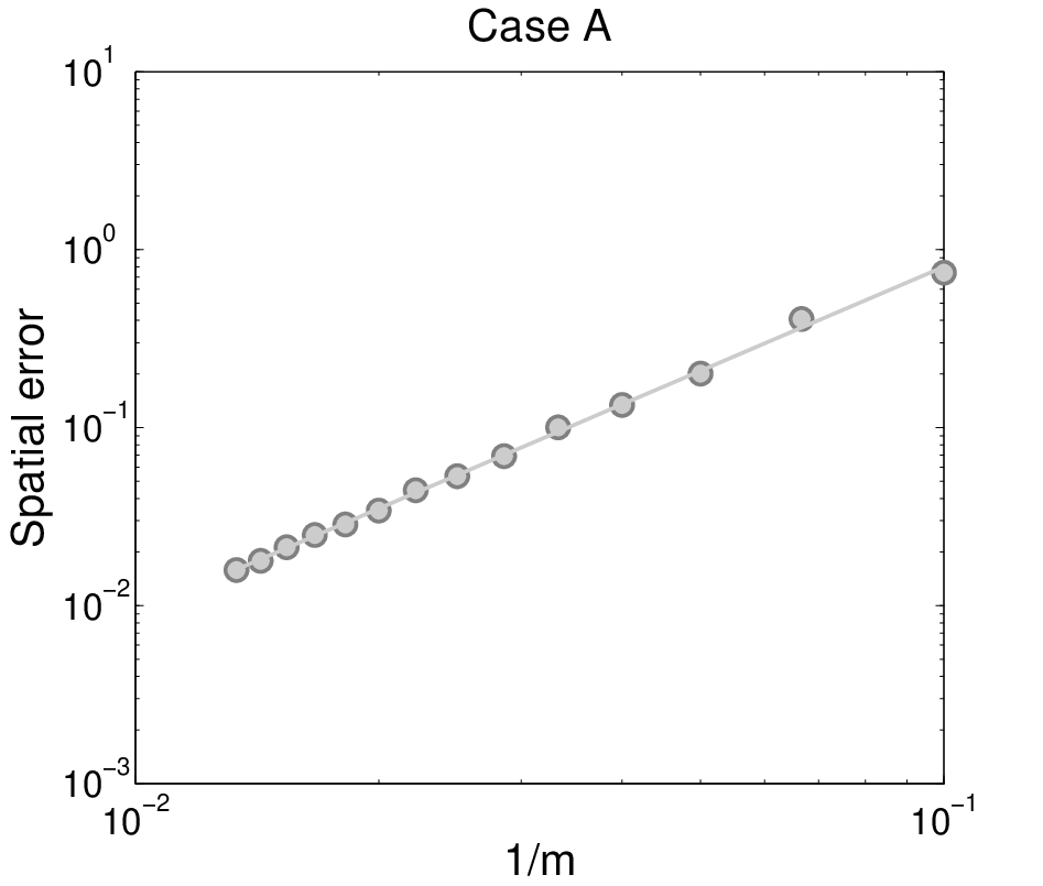
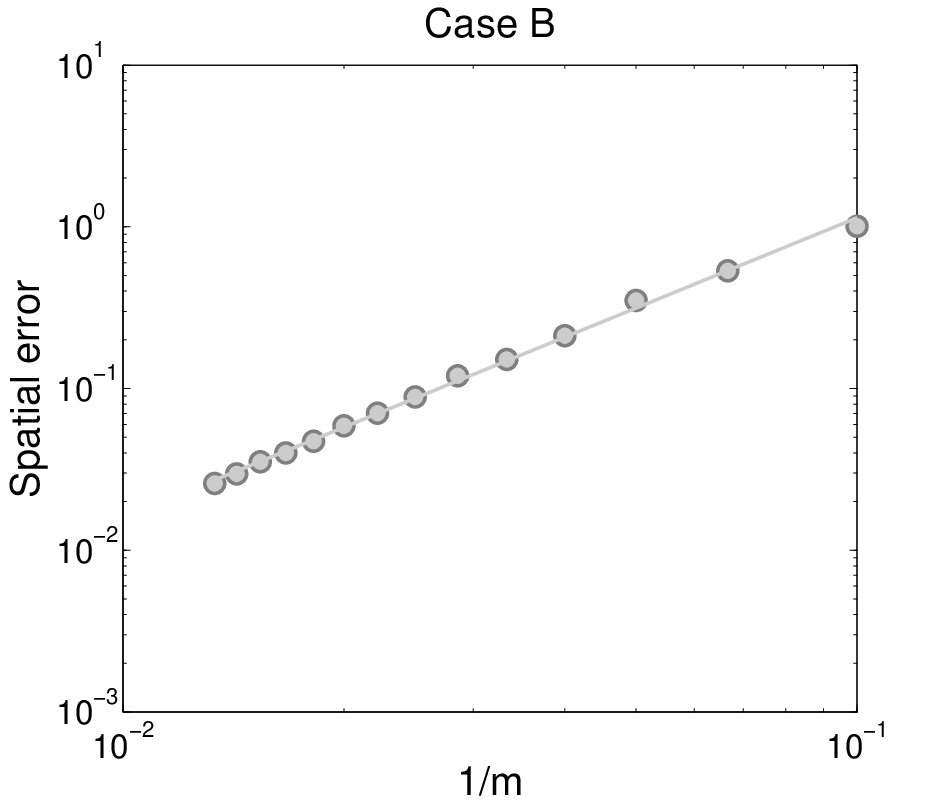
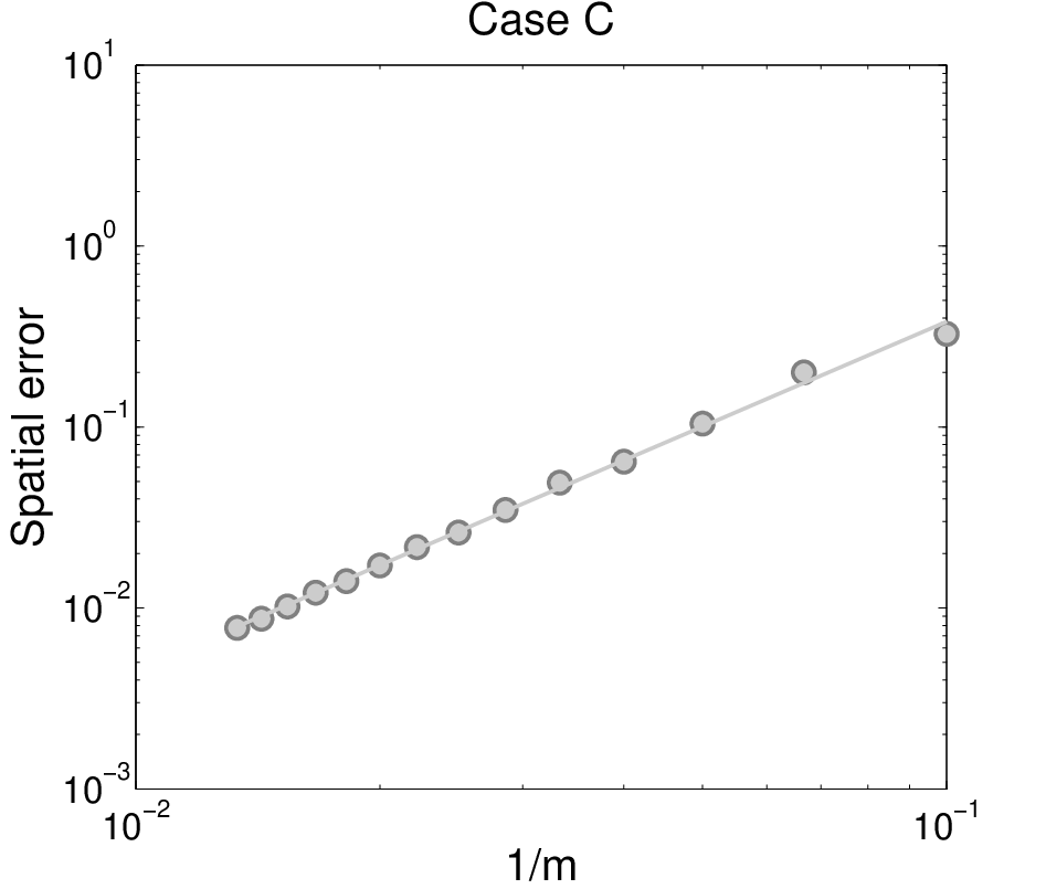
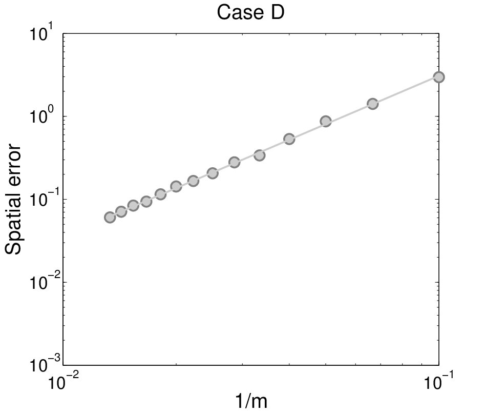
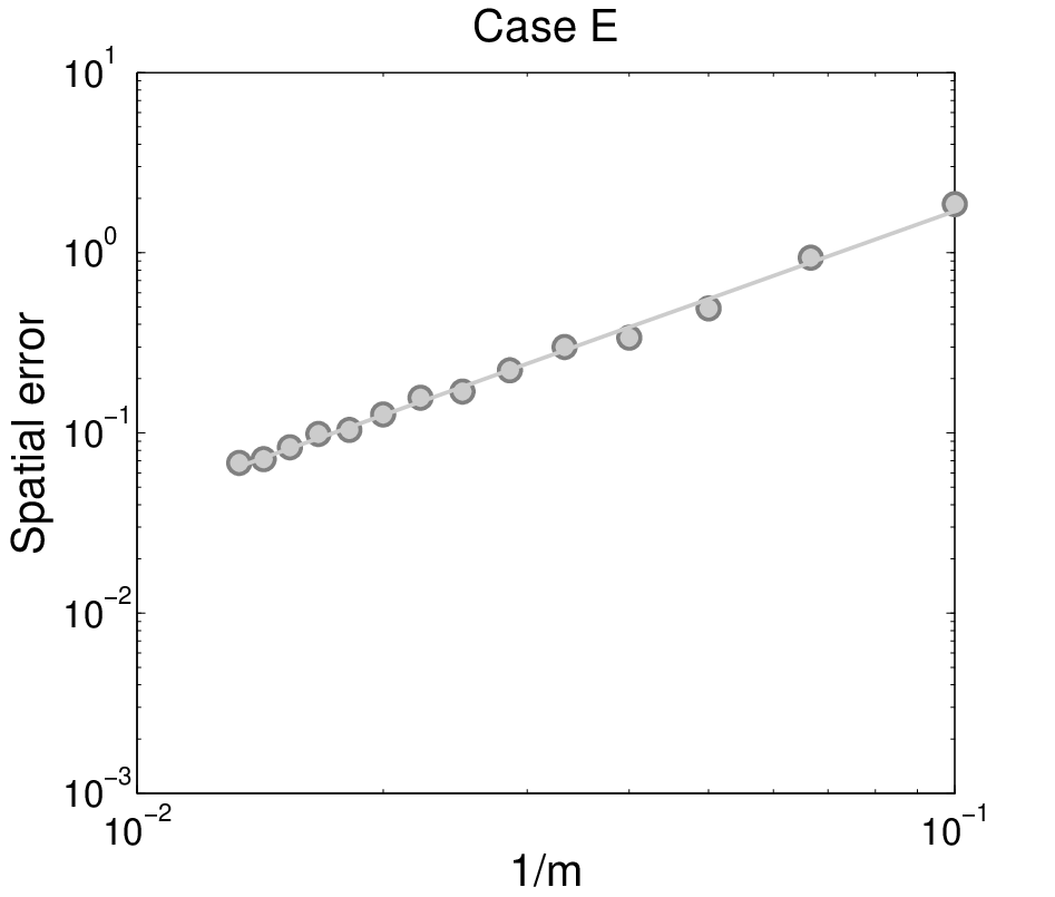
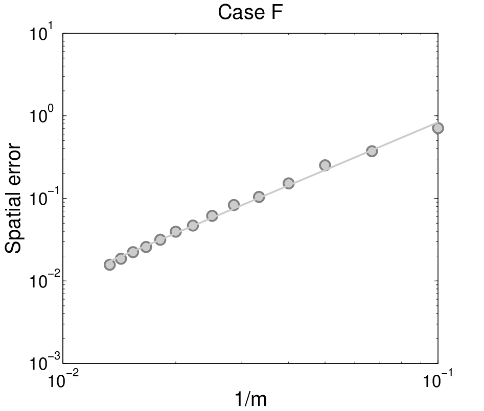
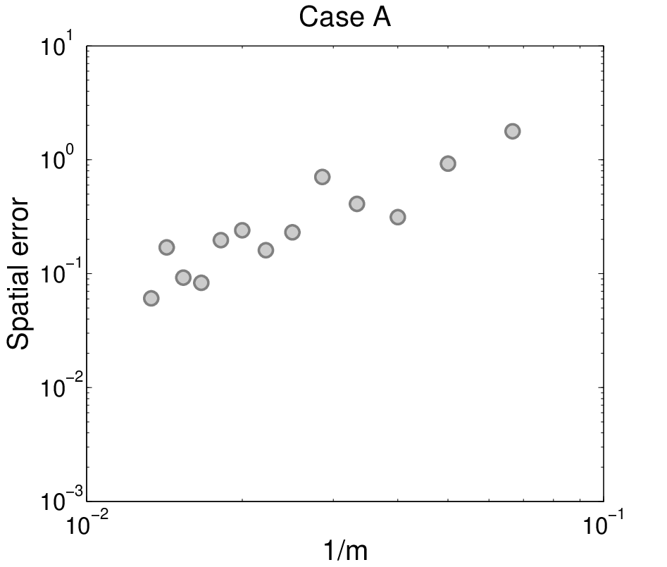
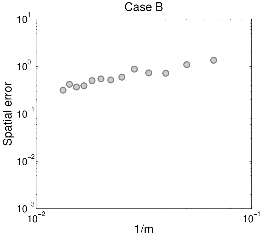
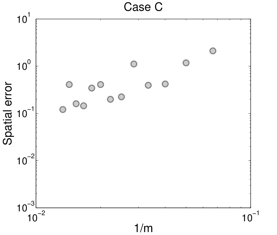
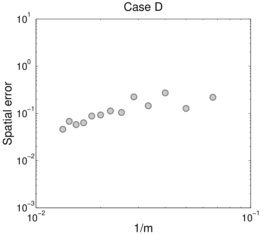
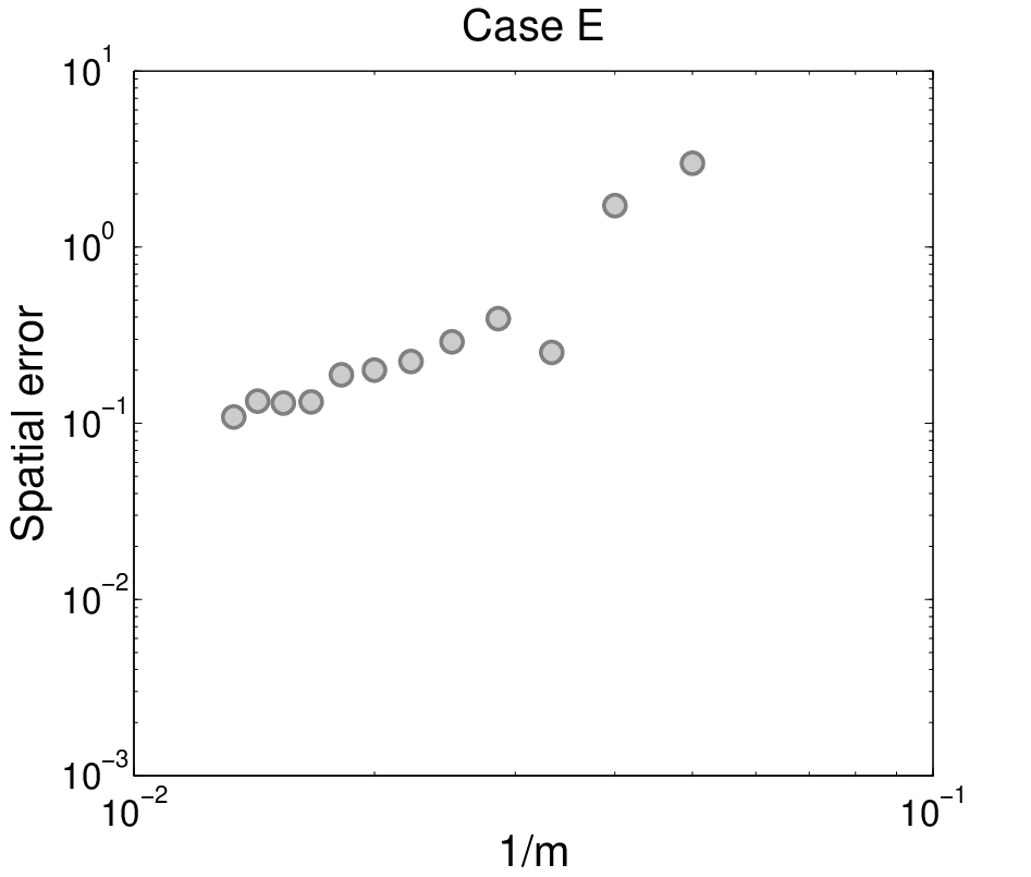
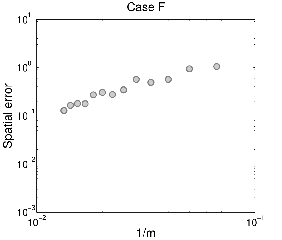
As mentioned above, it is possible to compute these whenever . Figure 2 displays the errors vs in the six pertinent cases of Table 1 for . Note that means spatial grid points, which was the practical (memory) limit on our laptop computer. Figure 2 clearly shows that in each case the spatial discretization errors decrease as increases. To determine the numerical orders of convergence, straight lines have been fitted to the results. In the cases A, B, C, D, F the obtained orders of convergence are all equal to two approximately. Only in case E a slightly lower order was obtained, namely 1.6. As an indication of the sizes of the spatial discretization errors in a relative sense, we mention that these always lie between 0.2% and 1.2% when and between 0.1% and 0.6% when (here only option values are considered that are greater than 1). In view of the foregoing, we conclude that the FD discretization defined in Section 2 performs satisfactory in all six cases. It is interesting to briefly compare the spatial errors to those obtained with a uniform grid and the same number of grid points. Figure 3 shows spatial discretization errors analogously to Figure 2, but then for uniform grids. Clearly, in most cases the spatial errors for the nonuniform grid are substantially smaller, often by an order of magnitude, than those for the corresponding uniform grid. Further, it is clear that for a uniform grid the behavior of the spatial error as a function of the number of grid points is erratic, which is undesirable. Also, the nonuniform grid yields more points in the region in –space where one wishes to obtain option prices. We therefore conclude that the nonuniform grid defined in Section 2 is preferable over a uniform grid.
 |
 |
 |
 |
 |
 |
We next consider the performance of the four ADI schemes in the application to the semidiscrete HHW PDE for European call options in the six cases of Table 1 with all correlations nonzero. Figure 4 displays the temporal discretization errors for a sequence of step sizes with when .
A first main observation from Figure 4 is that for all four ADI schemes the temporal discretization errors are bounded from above by a moderate value and decay monotonically as decreases. Additional experiments indicate that this is true for any value ; see a further discussion below. This suggests an unconditionally stable behavior of the schemes, which is a new and nontrivial result. It does not directly follow for example from the von Neumann stability analysis presented in Section 3. We note that this result holds in all six cases, independently of whether or not the Feller condition is fulfilled.
A next observation is that the CS scheme exhibits an undesirable feature in the cases A, B, C with temporal errors that are very large for moderate , compared to what may be expected on the basis of its asymptotic error behavior (ie, for small ). To a much lesser extent, this is also observed with the HV and MCS schemes. Additional experiments reveal that the relatively large temporal errors occur at spatial grid points near the strike . It is already known in the literature that the nonsmoothness of the initial function at the strike yields high-frequency errors which are not always sufficiently damped by numerical schemes, notably the Crank–Nicolson scheme and the Do and CS schemes with . A popular remedy for this situation is to first apply, at , two implicit Euler steps with step size , and then to proceed onwards from with the scheme under consideration, cf Rannacher (1984). However, in our present application of the three-dimensional HHW PDE this damping procedure is computationally intensive. We shall consider an alternative in the next subsection.
A further analysis of the results in Figure 4 indicates that in each case the temporal discretization errors for the Do scheme are bounded from above by and for the MCS, HV schemes by (whenever ) with constants depending on the scheme and the case. This clearly agrees with the respective orders of consistency of the schemes. Moreover, experiments with both smaller and larger values of suggest that the constants are only weakly dependent on the number of spatial grid points , ie, the error bounds are valid in a stiff sense, which is a desirable property. This result is also nontrivial, as the order of consistency is a priori only relevant to fixed, nonstiff systems of ODEs. For the CS scheme, we find that the temporal errors can be bounded in each case by with a constant independent of stiffness if damping is applied. Actual numerical experiments for ADI schemes combined with damping will be presented in the next subsection.
Our implementation of the ADI finite difference discretization has been done in Matlab, where all matrices have been defined as sparse. For the CS, MCS, HV schemes the cpu-time per time step was about 0.10, 0.18, 0.90, 1.5 cpu-seconds for 25, 30, 50, 60, respectively, on one Intel Core Duo T7250 2.00 GHz processor with 4 GB memory; for the Do scheme these times are about halved. Here all correlations were nonzero and the mean reversion level was time-dependent. It readily follows that the cpu-times are indeed almost directly proportional to the number of spatial grid points .
4.2 Up-and-out call options
As an important and particularly challenging type of exotic options we consider here European-style up-and-out call options. The FD discretization described in Section 2 is adapted with few modifications. Let barrier be given. Then the boundary conditions (2.1b), (2.1c) are replaced by
| (4.4) |
The condition (4.4b) has been suggested by various authors in the literature. Note that all boundary conditions are now homogeneous, and . The relevant set of spatial grid points is
The only significant change we make to the FD discretization of Section 2 is to replace, in the -direction, the central advection scheme (2.2b) by the backward scheme (2.2a) if and by the forward scheme (2.2c) if . This upwind approach alleviates spurious oscillations in the FD solution that are obtained with the central advection scheme. It is already useful for up-and-out call options in the one-dimensional Black–Scholes model. The pricing of up-and-out call options is numerically more challenging than of vanilla options, due to the boundary layer that is introduced at the barrier.
 |
 |
 |
 |
 |
 |
 |
 |
 |
 |
 |
 |
 |
 |
 |
 |
 |
 |
Figure 5 displays the numerically obtained up-and-out call option values in the six cases of Table 1 for barrier and (sampled) spot interest rates on the -domain . Here the FD discretization has been applied with and for the time discretization the HV scheme is used with .
We study in detail the performance of the four ADI schemes. Similar to the case of European call options, Figure 6 shows the temporal discretization errors in the case of up-and-out call options for a sequence of step sizes when . As a first observation, it is clear from Figure 6 that the unfavorable feature of relatively large temporal errors for moderate step sizes is more pronounced compared to the case of vanilla options, especially for the CS scheme, cf Subsection 4.1. We attribute this to the additional discontinuity of the payoff function at the barrier . We therefore consider application of a damping procedure at . Instead of performing two substeps at with step size by the implicit Euler scheme, which forms a common approach, we employ here the Do scheme, with parameter value . This is computationally more attractive when dealing with multidimensional PDEs. Figure 7 shows the temporal discretization errors in the case of up-and-out call options when two initial substeps with the Do scheme and are applied. Clearly, the behavior of the temporal error as a function of the step size has become regular and, in most cases, at only a limited loss of accuracy for small (an exception being the CS scheme in case E). Hence, the present damping procedure performs satisfactory. Applying two substeps of the implicit Euler scheme for the damping would yield similar or somewhat smaller temporal errors than those in Figure 7. However, we find that this comes at a much higher computational cost, also when iterative solvers, like BiCGSTAB, are applied. We thus infer that damping with the Do scheme is more efficient.
As a main positive conclusion, the numerical results for all ADI schemes are consistent with an unconditionally stable behavior: the temporal discretization errors are bounded from above by a moderate value and decay monotonically as decreases, which is obtained for any value tested. A closer inspection of the results displayed in Figure 7 yields that the temporal errors behave for sufficiently small as with for the Do scheme and for the CS, MCS, HV schemes, with constants . Experiments with different values of reveal that both and are only weakly dependent on the number of spatial grid points , indicating that the error behavior is valid in a stiff, hence favorable, sense. Note further that the difference in performance between the Do scheme and the CS, MCS, HV schemes is often less striking than in the case of vanilla options, but for the latter three schemes combined with damping still a higher order and increased accuracy is obtained.
5 Conclusions and future research
In this paper we studied ADI schemes in the numerical solution of the three-dimensional HHW PDE: the Do scheme, the CS scheme, the MCS scheme and the HV scheme, each with a well chosen parameter . Extensive experiments have been conducted for six cases of parameter sets for the HHW model, including correlations that are all nonzero, time-dependent mean-reversion levels, and short and long maturities. In three cases the Feller condition is not fulfilled. We considered both European call options and up-and-out call options. Our tests have shown that all ADI schemes perform very well in terms of stability, accuracy and efficiency. In particular they always reveal an unconditionally stable behavior. Next, the Do scheme always has a stiff order of convergence equal to one. The CS, MCS, HV schemes show a stiff order of convergence equal to two for European call options and, when combined with damping, between 1.6 and 2.0 for up-and-out call options.
Based on the numerical experiments and the theoretical stability results, we find that the MCS scheme with and the HV scheme with are preferable. Here . Also the CS scheme with is a good candidate. For the latter scheme, a damping procedure at is always recommended. Damping can be done efficiently, in an ADI fashion, by applying the Do scheme with .
The Do, CS, MCS and HV schemes are expected to perform well and possess similar favorable properties as obtained in this paper in the numerical solution of many other three-dimensional PDEs and for other exotic options. Also, the ADI schemes can directly be applied, with high efficiency, when any other FD discretization is employed, as the matrices () always have a small bandwidth. We shall investigate other applications in future research. At the same time, a further theoretical stability analysis of the ADI schemes will be carried out.
Appendix
Here we give the semi closed-form analytic formula for European call option values under the HHW model (1.1) with as derived in Muskulus, In ’t Hout, Bierkens et al (2007). The notation is adapted to our present situation. We put .
The solution presented in loc cit is of a form similar to the Black–Scholes formula,
Here denotes the value at time of a zero-coupon bond that pays 1 at maturity, given that at time the short rate equals . For this, it is well-known that
| (5.1) |
The , can be viewed as probabilities and are retrieved from characteristic functions , by inversion:
with . The functions , have the form
Let , and . Then
Next, let
and
Then
Finally,
The above valuation formula is easily seen to constitute a proper extension of Heston’s (1993) formula, by taking and . It can be approximated to any accuracy, by a direct adaptation of numerical integration techniques already well studied in the literature for Heston’s formula. We note that the additional integrals involving the function can be exactly determined in our particular case of (4.3).
Acknowledgements
The authors gratefully acknowledge Peter Forsyth for a stimulating discussion, convincing them of the proper boundary condition for the HHW PDE at and pointing them to the work by Ekström & Tysk. The authors also thank Jan Van Casteren for a valuable, unpublished note on the validity of the HHW PDE. Furthermore, they are indebted to Sven Foulon for providing an implementation of Heston’s formula for European call options, which we extended to our case. This work has been supported financially by the Research Foundation – Flanders, FWO contract no. G.0125.08.
References
- [1] L. Andersen, Simple and efficient simulation of the Heston stochastic volatility model, J. Comp. Finan. 11 (2008) 1–42.
- [2] L. Andersen & J. Andreasen, Jump-diffusion processes: volatility smile fitting and numerical methods for option pricing, Rev. Deriv. Research 4 (2000) 231–262.
- [3] L. B. G. Andersen & V. V. Piterbarg, Interest Rate Modeling, Volume I: Foundations and Vanilla Models, 1st ed., Atlantic Financial Press, 2010.
- [4] Bloomberg Quant. Finan. Devel. Group, Barrier options pricing under the Heston model, 2005.
- [5] I. J. D. Craig & A. D. Sneyd, An alternating-direction implicit scheme for parabolic equations with mixed derivatives, Comp. Math. Appl. 16 (1988) 341–350.
- [6] D. M. Dang, C. C. Christara, K. R. Jackson & A. Lakhany, A PDE pricing framework for cross-currency interest rate derivatives, Proc. 10th Int. Conf. Comp. Sc. (ICCS), Proc. Comp. Sc. 1 (2010) 2371–2380.
- [7] D. Egloff, GPUs in financial computing part III: ADI solvers on GPUs with application to stochastic volatility, Wilmott mag., March 2011, 51–53.
- [8] E. Ekström & J. Tysk, Boundary conditions for the single-factor term structure equation, Ann. Appl. Prob. 21 (2011) 332–350.
- [9]
A. Giese,
On the pricing of auto-callable equity structures in the
presence of stochastic volatility and stochastic interest rates,
presentation MathFinance Workshop, Frankfurt (2006).
Available at www.mathfinance.com/workshop/2006/papers/giese/slides.pdf - [10] L. A. Grzelak & C. W. Oosterlee, On the Heston model with stochastic interest rates, SIAM J. Finan. Math. 2 (2011) 255–286.
- [11] L. A. Grzelak, C. W. Oosterlee & S. van Weeren, Extension of stochastic volatility equity models with the Hull–White interest rate process, published online in Quant. Finan. (2009), doi:10.1080/14697680903170809.
- [12] T. Haentjens & K. J. in ’t Hout, ADI finite difference discretization of the Heston–Hull–White PDE, In: Numerical Analysis and Applied Mathematics, eds. T. E. Simos et al, AIP Conf. Proc. 1281 (2010) 1995–1999.
- [13] S. L. Heston, A closed-form solution for options with stochastic volatility with applications to bond and currency options, Rev. Finan. Stud. 6 (1993) 327–343.
- [14] K. J. in ’t Hout, ADI schemes in the numerical solution of the Heston PDE, In: Numerical Analysis and Applied Mathematics, eds. T. E. Simos et al, AIP Conf. Proc. 936 (2007) 10–14.
- [15] K. J. in ’t Hout & S. Foulon, ADI finite difference schemes for option pricing in the Heston model with correlation, Int. J. Numer. Anal. Mod. 7 (2010) 303–320.
- [16] K. J. in ’t Hout & C. Mishra, A stability result for the Modified Craig–Sneyd scheme applied to 2D and 3D pure diffusion equations, In: Numerical Analysis and Applied Mathematics, eds. T. E. Simos et al, AIP Conf. Proc. 1281 (2010) 2029–2032.
- [17] K. J. in ’t Hout & C. Mishra, Stability of the modified Craig–Sneyd scheme for two-dimensional convection-diffusion equations with mixed derivative term, Math. Comp. Simul. 81 (2011) 2540–2548.
- [18] K. J. in ’t Hout & B. D. Welfert, Stability of ADI schemes applied to convection-diffusion equations with mixed derivative terms, Appl. Numer. Math. 57 (2007) 19–35.
- [19] K. J. in ’t Hout & B. D. Welfert, Unconditional stability of second-order ADI schemes applied to multi-dimensional diffusion equations with mixed derivative terms, Appl. Numer. Math. 59 (2009) 677–692.
- [20] J. Hull & A. White, Pricing interest-rate-derivative securities, Rev. Finan. Stud. 3 (1990) 573–592.
- [21] W. Hundsdorfer & J. G. Verwer, Numerical Solution of Time-Dependent Advection-Diffusion-Reaction Equations, Springer, Berlin, 2003.
- [22] A. Itkin & P. Carr, Jumps without tears: a new splitting technology for barrier options, Int. J. Numer. Anal. Mod. 8 (2011) 667–704.
- [23] D. Lanser, J. G. Blom & J. G. Verwer, Time integration of the shallow water equations in spherical geometry, J. Comp. Phys. 171 (2001) 373–393.
- [24] A. Lipton, Mathematical Methods for Foreign Exchange, World Scientific, Singapore, 2001.
- [25] S. McKee & A. R. Mitchell, Alternating direction methods for parabolic equations in two space dimensions with a mixed derivative, Computer J. 13 (1970) 81–86.
- [26] M. Muskulus, K. J. in ’t Hout, J. Bierkens, A. P. C. van der Ploeg, J. in ’t Panhuis, F. Fang, B. Janssens & C. W. Oosterlee, The ING problem: a problem from the financial industry, Proc. 58th European Study Group Mathematics with Industry, eds. R. H. Bisseling et al, Utrecht (2007) 91–115.
- [27] C. Randall, PDE Techniques for Pricing Derivatives with Exotic Path Dependencies or Exotic Processes, Lecture notes, Workshop CANdiensten, Amsterdam, 2002.
- [28] R. Rannacher, Finite element solution of diffusion problems with irregular data, Numer. Math. 43 (1984) 309–327.
- [29] W. Schoutens, E. Simons & J. Tistaert, A perfect calibration! Now what?, Wilmott mag., March 2004, 66–78.
- [30] D. Tavella & C. Randall, Pricing Financial Instruments, Wiley, New York, 2000.
- [31] G. Winkler, T. Apel & U. Wystup, Valuation of options in Heston’s stochastic volatility model using finite element methods, in: Foreign Exchange Risk, eds. J. Hakala & U. Wystup, Risk Books, London (2002) 283–303.