Quantum phase transitions in the Kane-Mele-Hubbard model

In order to simplify the implementation, the trial wave function is taken to be a single Slater determinant, and can hence always be written in terms of the groundstate of a single-particle Hamiltonian $H_{\text{T}}$. There are many possible choices for $\left|\Psi_{\text{T}}\right\rangle$. One can for example decide to optimize the overlap with the groundstate at the expense of symmetries.[22] Here we have preserved symmetries, and have chosen $|\Psi_{\text{T}}\rangle$ to be the groundstate of the KM model, which is defined by the first line of Eq. (1). For $\lambda\neq 0$, the groundstate of the noninteracting problem at half filling is insulating. Hence, the trial wave function is nondegenerate and has all the symmetries of the Hamiltonian. At $\lambda=0$, the situation is more delicate. For the considered lattice sizes, $L=3l$, the two nonequivalent Dirac points are located at the Fermi surface, and the groundstate of the noninteracting model at half filling is four-fold degenerate in each spin sector. We lift this degeneracy by means of a twist in the boundary condition in $H_{\text{T}}$ in the direction $\bm{a}_{1}=(1,0)$,

with $\bm{A}=\Phi\bm{a}_{1}/L$. The twist preserves translation symmetry, so that the total momentum remains a good quantum number. In particular, for an infinitesimal twist, the groundstate has vanishing total momentum. Because finite values of $\Phi$ lead to a breaking of the $C_{3}$ lattice symmetry, the trial wave function cannot be classified according to the irreducible representation of this group at $\lambda=0$. After lifting possible degeneracies, $|\Psi_{\text{T}}\rangle$ corresponds to the nondegenerate groundstate of $H_{\text{T}}$. This implies the relation

where $E_{\text{T}}$ is the corresponding groundstate energy.

We choose a HS transformation of the Hubbard term $H_{U}$ that couples to the total density $n_{i}=n_{i\uparrow}+n_{i\downarrow}$, thereby conserving the $SU(2)$ spin symmetry for every field configuration. In principle, HS transformations that couple to the $z$-component of spin are also possible. However, at low temperatures, it is often difficult to restore the $\lambda=0$ $SU(2)$ spin symmetry of the total Hamiltonian by stochastic sampling. An $SU(2)$ spin symmetric transformation was previously used in Refs. 23, 24.

After a Trotter decomposition with imaginary time step $\Delta\tau$ to isolate the interaction term, our HS transformation for a general operator $O$ reads

with the two functions $\gamma(l)$ and $\eta(l)$ of the auxiliary field $l$ (with $l=\pm 1,\pm 2$) taking on the values

Equation (5) is an approximation to the Gaussian integral and introduces an overall systematic error of the order $\Delta\tau^{3}$, which is negligible in comparison to the Trotter error of order $\Delta\tau^{2}$. The major advantage of this approximation is that we can avoid using continuous auxiliary fields while retaining spin rotation symmetry. For the Hubbard interaction, we have $O=\sqrt{U/2}(n_{\uparrow}+n_{\downarrow}-1)$ and it is understood that the HS fields acquire space and time indices, $l\mapsto l_{\bm{i},\tau}$.

We prove the absence of the minus-sign problem for the projective QMC method at half filling. With the Trotter decomposition, choice of trial wave function and HS transformation, the denominator of Eq. (2) factors into spin-up and spin-down determinants,

where we have used Eq. (4) to introduce a trace, $\{l_{\bm{i},\tau}\}$ denotes an auxiliary-field configuration, and with the weights

Here we introduced the notation $H_{\text{T}}=\sum_{\bm{ij}\sigma}c^{\dagger}_{\bm{i}\sigma}[h^{\phantom{{\dagger}}}_{\text{T}}(\Phi)]^{\phantom{{\dagger}}}_{\bm{ij}}c^{\phantom{{\dagger}}}_{\bm{j}\sigma}$ and $H_{\text{KM}}=\sum_{\bm{ij}\sigma}c^{\dagger}_{\bm{i}\sigma}(A_{t}+A_{\lambda,\sigma})^{\phantom{{\dagger}}}_{\bm{ij}}c^{\phantom{{\dagger}}}_{\bm{j}\sigma}$. Proving the absence of a negative sign problem at half filling amounts to showing that $W_{\uparrow}^{*}=W_{\downarrow}$. Since the trace in Eq. (8) is over one spin sector, we drop the spin index on the fermion operators to lighten the notation and obtain

The second line follows from the canonical transformation $c^{\phantom{{\dagger}}}_{\bm{i}}\rightarrow(-1)^{\bm{i}}c^{\dagger}_{\bm{i}}$, where the phase factor $(-1)^{\bm{i}}$ takes the value $1$ ($-1$) on sublattice A (B). The Hamiltonian $H_{\text{T}}$ which generates the trial wave function has nonvanishing matrix elements only between sites on opposite sublattices. Hence $(-1)^{\bm{i}+\bm{j}}=-1$ and

Similarly, for the hopping term,

Since the spin-orbit term involves hopping between sites on the same sublattice, we have

Using Eqs. (10)–(12), one sees that indeed

so that no sign problem exists at the particle-hole symmetric point of the KMH model in the present formulation of the QMC algorithm.[7] The underlying reason is time reversal symmetry, which implies $A_{\lambda,\downarrow}=-A_{\lambda,\uparrow}$.

For a given auxiliary-field configuration, we have to solve a free-electron Hamiltonian with external fields that vary in time and space. Consequently, Wick’s theorem holds, and it is sufficient to compute the single-particle Green functions

to calculate arbitrary correlation functions. For the calculation of $G_{\sigma}$ we have followed Ref. 25. The single-particle gap $\Delta_{\text{sp}}$ at the Dirac point and the (staggered) spin gap $\Delta_{\text{s}}$ at $\bm{q}=0$ are extracted from fits to the corresponding Green functions.[6]

The projective algorithm involves two numerical parameters, namely the projection parameter $\theta$ and the Trotter time step $\Delta\tau$. Both parameters were chosen such that their influence on the results is smaller than the statistical errors. Explicitly, we used $\Delta\tau t=0.05$ or 0.1, and $\theta t=40$–$60$.

Figure 1 shows the groundstate phase diagram of the KMH model, as obtained from QMC simulations. In addition to the three phases of the Hubbard model on the honeycomb lattice, the spin-orbit coupling introduces a $Z_{2}$ TBI. The gapless SM phase exists only at $\lambda=0$. Whereas the TBI and the QSL phase are fully gapped (finite single-particle gap $\Delta_{\text{sp}}$ and spin gap $\Delta_{\text{s}}$), the magnetic phase has $\Delta_{\text{sp}}>0$ but $\Delta_{\text{s}}=0$. Here all gaps refer to the bulk, and are not to be confused with the metallic, gapless edge states of the TBI phase of the KMH model.

To the best of our knowledge, the QSL phase is characterized by the absence of any local order parameter which would reflect a broken-symmetry state. It can hence be regarded as a genuine Mott insulating state, which should be stable with respect to small perturbations such as spin-orbit coupling. In the case of an odd number of electrons per unit cell, the generalization of the Lieb-Schultz-Mattis theorem to two dimensions[26] suggests the presence of topological order in the most general sense. Since the half-filled honeycomb lattice has two electrons per unit cell, this topological ordering still has to be numerically demonstrated or refuted. The underlying $SU(2)\times SU(2)/Z_{2}$ symmetry of the Hubbard model on the honeycomb lattice has led to the prediction of a $Z_{2}\times Z_{2}$ QSL with mutual spin-charge statistics.[27] Sublattice pairing states have been put forward by various authors to account for the QSL phase.[28, 29] A canonical consequence of the above topologically ordered phases is that, assuming a continuous phase transition, the magnetically ordered phase would not be a simple Néel state, thus leading to conjectures that can be tested numerically.[28, 29] Finally, in the presence of spin-orbit coupling, the possibility of the emergence of a topological Mott insulating phase, in which the spinons carry the topological character of the phase, remains.[30, 31] For the KMH model, recent theoretical suggestions include a $Z_{2}$ QSL[15] and a chiral QSL.[20]

The boundary of the magnetic phase is obtained from the onset of long-range antiferromagnetic order in the $xy$ plane. Longitudinal order, present at $\lambda=0$, can be excluded in Fig. 1 for all $U/t$ and for $\lambda/t\geq 0.002$, so that the $xyz$ AFMI phase is confined to a very small (possibly infinitesimal) interval starting at $\lambda=0$. The SM–TBI transition is evinced by the simultaneous opening of a single-particle and a spin gap, which as a function of $\lambda$ closely follow the $U=0$ results. The QSL–TBI transition for intermediate Hubbard $U$ and small $\lambda$ turns out to be the most difficult and perhaps most interesting case, with the critical values extracted from a cusp (consistent with a closing) of the single-particle gap $\Delta_{\text{sp}}$ and the spin gap $\Delta_{\text{s}}$. A more detailed discussion is given below.

Our numerical results suggest that the TBI phase at finite $U$ is adiabatically connected to the TBI state of the KM model ($U=0$). Similarly, the QSL phase is stable over a finite range of $\lambda$, in accordance with theoretical predictions.[15] Except for the smaller range of spin-orbit couplings compared to Ref. 7, which is chosen here to highlight the structure of the phase diagram around the QSL, we have obtained a number of additional points for the phase boundary of the QSL. The refined QSL phase boundary reveals a direct magnetic transition between the QSL and the AFMI phase at finite $\lambda$. Our numerical data suggest the existence of a multicritical point where the QSL, TBI and AFMI phases meet. The estimated location of this point is $(\lambda_{\text{c}},U_{\text{c}})\approx(0.035t,4.2t)$.

Let us compare the phase diagram in Fig. 1 to other work. The magnetic phase boundary was calculated using mean-field theory.[9] In that work, a transition from the TBI to an AFMI phase is observed, with the critical $U$ increasing with increasing $\lambda$ and comparable to the band width. However, the numerical values differ by up to a factor of two. The phase diagram from unbiased QMC simulations was presented by three of us.[7] At that time, only one point on the QSL–TBI phase boundary was available, and the suggested dome-like structure of the QSL phase was based on the fact that the spin gap takes on its maximum around $U/t=4$, in the middle of the $\lambda=0$ QSL phase. Soon after this work, QMC results for the phase diagram were published by Zheng et al. [8] Except for the absence of the QSL–TBI phase boundary, their phase diagram is compatible with previous[7] and current results (Fig. 1). The line $\lambda/t=0.1$ was studied by Yamaji and Imada using variational QMC simulations,[12] although with rather large quantitative differences concerning the location of the TBI–AFMI transition. The phase diagram has also been calculated using the variational cluster approach,[10] and cluster dynamical mean-field theory.[11] Apart from the fact that a true QSL phase is not accessible in any cluster calculation, the overall structure of the phase diagram in these works is consistent with Fig. 1. The quantitative phase boundaries seem to be slightly more accurate in the cluster dynamical mean-field case.[11] Both papers show a “QSL”–TBI phase boundary whose shape is in accordance with our refined phase diagram in Fig. 1.

Lee[14] and Griset and Xu[15] have recently made predictions about the nature of some of the phase transitions. In both works, the TBI–AFMI transition is argued to be in the 3D XY universality class, as already hinted at in Ref. 7. Griset and Xu further suggest that both the QSL–AFMI and the QSL–TBI transitions could be first order quantum phase transitions.[15] They also highlight the possibility of an additional, nematic order-disorder transition inside the AFMI at $\lambda=0$, instead of a proposed chiral AF order-disorder transition in the Hubbard model[29] that should persist also at $\lambda>0$.[15] The phase diagram of the KMH model has also been calculated using analytical methods.[19, 20]

With the number of phases and their boundaries being rather well established, the important open questions about the phase diagram concern the nature of the QSL and AFMI phases, and of the various phase transitions. The structure of the phase diagram implies the existence of several distinct quantum phase transitions: SM–TBI, TBI–AFMI, QSL–AFMI, and QSL–TBI. The remaining SM–QSL transition only occurs at $\lambda=0$, and has been studied in detail before.[6] We discuss each of these transitions below.

The remainder of this section is organized as follows. We first consider the SM–TBI transition (at fixed $U/t=2$, see Fig. 1) and the TBI–AFMI transition (at fixed $\lambda/t=0.1$), for which we can provide a fairly complete picture. From this we move on to the QSL–AFMI transition (considering $\lambda/t=0.0125$), and finally the QSL–TBI transition (at $U/t=4$).

We begin with the SM–TBI transition. To this end, we keep $U/t=2$ fixed. In the absence of interactions, the spin-orbit term breaks the sublattice symmetry and generates a mass gap as well as a topological band structure. Due to the underlying $U(1)$ spin symmetry, the band structure corresponds to two Haldane models with Chern numbers of opposite sign in the two spin sectors.[4]

Figure 2(a) shows QMC results for the single-particle gap $\Delta_{\text{sp}}$ and the spin gap $\Delta_{\text{s}}$ as a function of $\lambda$ at $U/t=2$. Starting in the SM phase at $\lambda=0$, where both gaps are zero, $\Delta_{\text{sp}}$ and $\Delta_{\text{s}}$ become nonzero for any finite $\lambda$, and increase with increasing spin-orbit coupling. The QMC results at $U/t=2$ closely follow the corresponding gaps for the noninteracting case $U=0$,[5] $\Delta_{\text{sp}}=3\sqrt{3}\lambda$ and $\Delta_{\text{s}}=2\Delta_{\text{sp}}$. Interaction effects manifest themselves as a minor suppression of both gaps compared to their noninteracting values, especially at larger $\lambda/t$, and by the spin gap falling below $2\Delta_{\text{sp}}$.

From these results, we draw the following conclusions. First, the SM phase of the Hubbard model is unstable at finite $\lambda$, and hence only exists for $\lambda=0$, as indicated in Fig. 1. Second, the very small deviations in the dependence of the gaps on $\lambda$ compared to the noninteracting case suggest that the TBI phase at $U>0$ is essentially the same as at $U=0$, provided $U$ remains small enough to avoid the magnetic transition. This finding suggests that the two states are adiabatically connected. The minor role of bulk interactions inside the TBI phase may be regarded as a consequence of the single-particle energy gap,[1] and has been exploited to develop an effective model of the helical edges with a Hubbard $U$ only at the edge sites of a ribbon.[7, 32]

The results for $\Delta_{\text{sp}}$ and $\Delta_{\text{s}}$ in Fig. 2(a) are obtained from finite-size scaling, as shown for selected values of $\lambda/t$ in Figs. 2(b) and (c). Whereas $\Delta_{\text{sp}}$ shows the familiar monotonic decrease with increasing system size, the spin gap reveals an unusual finite-size scaling behavior. Deep in the TBI phase [e.g., the top curve in Fig. 2(c) corresponding to $\lambda/t=0.03$], $\Delta_{\text{s}}$ systematically increases with increasing system size $L$. For small $\lambda$ (for example, $\lambda/t=0.0125$) and small $L$, the scaling behavior is more complex, and only the system sizes beyond the crossover have been used in the extrapolation. The increase of $\Delta_{\text{s}}$ with increasing $L$ is a correlation effect; the spin gap is independent of $L$ for $U=0$. The observed increase of $\Delta_{\text{s}}$ with system size can be reproduced using first-order perturbation theory in $U$.

A possible physical explanation is inspired by the observation that for small $L$, $\Delta_{\text{s}}(L)<2\Delta_{\text{sp}}(L)$, see Figs. 2(b) and (c). In contrast, the extrapolated values almost match the relation for the noninteracting case, $\Delta_{\text{s}}\approx 2\Delta_{\text{sp}}$, as shown in Fig. 2(a). The strongly suppressed spin gap for small system sizes indicates pronounced particle-hole binding, driven by correlation-induced magnetic fluctuations. If the length scale of these fluctuations, which are a precursor of the magnetic transition at $U_{\text{c}}$, exceeds the system size, the spin gap is expected to be suppressed similar to the magnetic phase where $\Delta_{\text{s}}\to 0$ as $L\to\infty$. Increasing $L$ beyond the correlation length will restore the behavior expected for the weakly or noninteracting TBI phase. We will see below (Fig. 9) that for larger $U/t=4$, the spin gap is suppressed to values much below $2\Delta_{\text{sp}}$ even in the thermodynamic limit. Although a complete understanding of this effect is currently missing, we regard the unusual spin gap scaling as a signature of a correlated TBI.

At large $U/t$, the TBI phase of the half-filled KMH model undergoes a transition to an AFMI, and TRI is spontaneously broken.[9] In the strong-coupling limit, $U/t\gg 1$, the charge degrees of freedom are frozen and one can derive an effective spin model with antiferromagnetic nearest-neighbor Heisenberg exchange $J=4t^{2}/U$ that promotes isotropic magnetic order in the $xy$ and $z$ directions. The spin-orbit term of the KMH model reduces the $SU(2)$ spin symmetry of the Hubbard model to a $U(1)$ symmetry corresponding to conservation of the total $z$-component of spin. Second-order perturbation theory gives an exchange interaction $J^{\prime}=4\lambda^{2}/U$ between next-nearest neighbors. Importantly, the exchange is antiferromagnetic in the longitudinal direction, $J^{\prime}S^{z}_{\bm{i}}S^{z}_{\bm{j}}$, but ferromagnetic in the transverse direction, $-J^{\prime}(S^{x}_{\bm{i}}S^{x}_{\bm{j}}+S^{y}_{\bm{i}}S^{y}_{\bm{j}})$.[9] Combining all the exchange terms, magnetic order in the $z$ direction becomes frustrated, and the system favors an easy-plane Néel state. The so-called KM-Heisenberg model was recently studied analytically.[20]

From the above considerations, $xy$ order is expected both for $\lambda=0$ and $\lambda\neq 0$. Hence, the phase boundary of the AFMI phase can be determined from the onset of transverse long-range magnetic order by monitoring the transverse structure factor

Here $\bm{r},\bm{r}^{\prime}$ denote unit cells, $\alpha,\beta\in\{A,B\}$ are sublattice indices, $(-1)^{\alpha}=1$ ($-1$) for $\alpha=A$ ($B$), and we have taken the trace of the corresponding $2\times 2$ matrix of the structure factor. The quantity $S_{\text{AF}}^{xy}/N$ (with $N=2L^{2}$) extrapolates to zero below $U_{\text{c}}(\lambda)$, but takes on a finite value in the thermodynamic limit for $U\geq U_{\text{c}}(\lambda)$, which is inside the AFMI phase of Fig. 1.[7, 8] It is also related to the transverse magnetization via $m_{xy}^{2}=S_{\text{AF}}^{xy}/N$.

Numerical results for $\lambda/t=0.1$ are shown in Fig. 3; the transition is most obvious from the extrapolated order parameter shown in the inset. The extrapolation of $S_{\text{AF}}^{xy}/N$ in system size gives a critical value $U_{\text{c}}/t=4.95(5)$. This value agrees with the slightly more accurate estimate $U_{\text{c}}/t=4.96(4)$ which follows from the intersect of curves for different system sizes in Fig. 5(a). However, this scaling analysis (see below for more details) relies on the knowledge of the universality class of the transition. By performing calculations at different $\lambda/t$, we can determine the magnetic phase boundary, and we find good agreement with previous exact simulations at $\lambda=0$[6] and $\lambda>0$.[7, 8] Our QMC results (not shown) further exclude the presence of longitudinal magnetic order along the entire TBI–AFMI phase boundary in Fig. 1 and up to $U/t=8$.

The TBI–AFMI transition is also reflected in the single-particle gap. Because the onset of long-range magnetic order at the TBI–AFMI transition spontaneously breaks TRI, the transition from the TBI to the nonadiabatically connected AFMI can in principle occur without closing any excitation gaps. Instead, the transition manifests itself in $\Delta_{\text{sp}}$ as a cusp at $U_{\text{c}}/t=4.95(5)$, visible in Fig. 4(a). The results are for the same value of $\lambda/t=0.1$ considered in Fig. 3. A similar signature can be reproduced already on the mean-field level, although with only a kink instead of a cusp at the critical point. Results for the gap and the mean-field order parameter are presented in the inset of Fig. 4(a). Figure 4(a) also shows the closing of the spin gap $\Delta_{\text{s}}$ at $U_{\text{c}}$; the results were obtained from the finite-size scaling shown in the inset of Fig. 6(a).

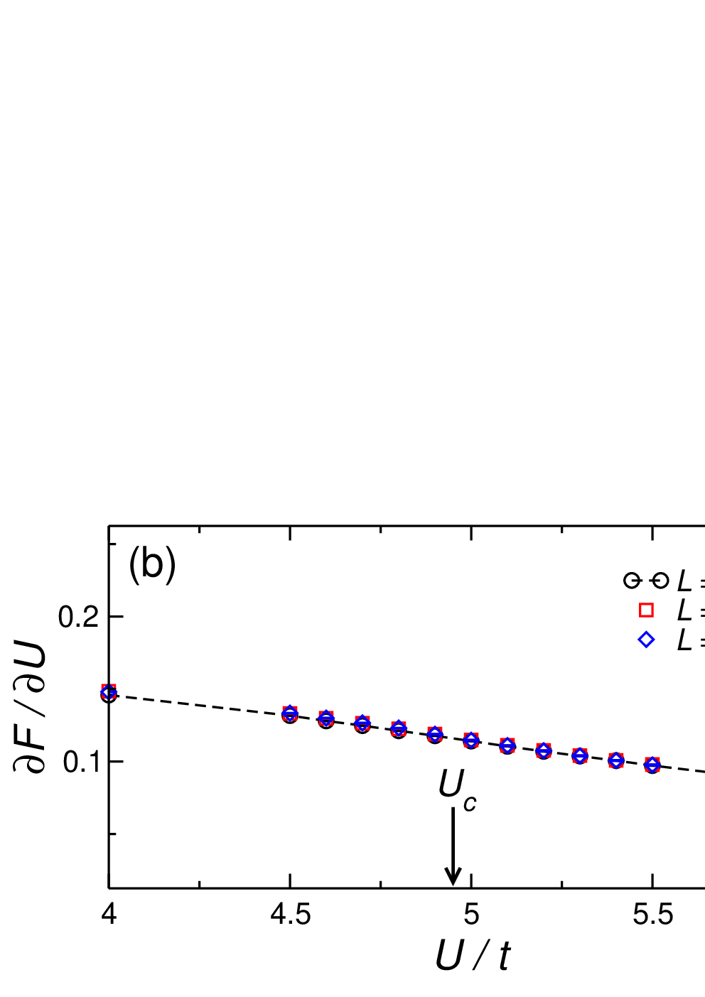
In Fig. 4(b), we present numerical data for the energy derivative

corresponding to the expectation value of the interaction term or, equivalently, the average double occupation, at $\lambda/t=0.1$. The continuous variation of this quantity across $U_{\text{c}}/t=4.95(5)$ suggests a continuous transition.

Having established the phase boundary of the magnetic transition at large $U/t$, we now consider the universality class. Given the remaining $U(1)$ spin symmetry in the presence of spin-orbit coupling, the transition is expected to be in the 3D XY universality class. An intuitive picture is based on local magnetic moments, which already exist in the magnetically disordered phase for $U>0$, and order at $U_{\text{c}}$. The onset of phase coherence at $U=U_{\text{c}}$ corresponds to a $U(1)$ symmetry breaking. This scenario is in accordance with the behavior of the spin gap $\Delta_{\text{s}}$ in Fig. 4. The excitons are massive in the disordered phase ($U<U_{\text{c}}$), but condense in the ordered phase ($U\geq U_{\text{c}}$) where $\Delta_{\text{s}}=0$.

The conjectured 3D XY universality can be tested using the zero-temperature, finite-size scaling forms

and

Here $f_{1}$ and $f_{2}$ are dimensionless functions. The relevant critical exponents for the 3D XY model are $z=1$, $\nu=0.6717(1)$ and $\beta=0.3486(1)$.[33]

Using the same value $\lambda/t=0.1$ as before, we show in Fig. 5(a) $L^{2\beta/\nu}S_{\text{AF}}^{xy}/N$ as a function of $U$ for different system sizes $L$. If the scaling form Eq. (17) with the critical exponents of the 3D XY model is correct, we expect to see an intersect of curves for different $L$ at $U=U_{\text{c}}$. As shown in Fig. 5(a), this prediction is indeed borne out by the QMC data, and we deduce $U_{\text{c}}/t=4.96(4)$, in agreement with Fig. 3. Replotting $L^{2\beta/\nu}S_{\text{AF}}^{xy}/N$ as a function of $L^{1/\nu}(U-U_{\text{c}})/U_{\text{c}}$ in Fig. 5(b) produces a clean scaling collapse onto a single curve. Figure 5 hence demonstrates that the assumption of 3D XY behavior is fully consistent with the QMC data.

Figure 6 shows a similar analysis for the spin gap $\Delta_{\text{s}}$, using the scaling form (18). Although the statistical quality of the data is not quite as good as for the structure factor, we again find satisfactory scaling (in particular, there is no noticeable drift of the intersect with increasing $L$) and the same $U_{\text{c}}$ using the 3D XY critical exponents.

Based on the existence of a $U(1)$ spin symmetry throughout the TBI phase, we expect the 3D XY behavior found at $\lambda/t=0.1$ to be generic for this transition, in agreement with previous predictions.[7, 15, 14] The finite-size corrections to the 3D XY scaling behavior become more pronounced on approaching the possible multicritical point, as verified explicitly for $\lambda/t=0.05$. According to Griset and Xu,[15] the observed 3D XY behavior at $\lambda>0$ suggests the absence of a chiral AF order-disorder transition inside the AFMI phase even for $\lambda=0$.[29]

The refined phase boundary of the QSL phase shown in Fig. 1 establishes the existence of a QSL–AFMI transition at finite $\lambda$, in addition to the $\lambda=0$ transition studied before.[6] Since the present work is concerned with the KMH model, we only consider finite values $\lambda>0$ here.

The simple picture of the magnetic transition as an ordering transition of magnetic moments (or exciton condensation) discussed in the context of the TBI–AFMI transition cannot straightforwardly be applied to the QSL–AFMI transition. For example, a $Z_{2}$ spin liquid exhibits charge fractionalization, and therefore has no well-defined magnetic modes. Fractionalization could lead to an unusually large anomalous dimension.[34] On the other hand, if the QSL phase was adiabatically connected to a simple band insulator (without charge fractionalization), the transition is again expected to be of the 3D XY type, similar to the TBI–AFMI transition.

Due to the small size of the spin gap in the QSL phase, the extrapolation of the order parameter (15) to the thermodynamic limit is much more delicate than for the TBI-AFMI transition. In particular, a scaling analysis along the lines of Figs. 5 and 6 is not conclusive with the currently available system sizes.

We first address the question of longitudinal magnetic order. The phase diagram presented by Yu et al.,[10] based on results from the variational cluster approach, shows an extended region inside the AFMI phase in which the authors claim that magnetic order exists both in the $xy$ plane and in the $z$ direction. For $\lambda=0$, this region is argued to extend all the way to the QSL–AFMI phase boundary, leading to a simultaneous onset of transverse and longitudinal order at $U_{\text{c}}$. At $\lambda>0$, Yu et al. [10] find a transition from the TBI to an $xy$ ordered AFMI at $U_{\text{c}}$, and an onset of $z$ order at even larger values of $U$. Hence, for $\lambda>0$, there would be an additional crossover (no symmetry breaking) inside the AFMI phase. Whereas $z$ order is known to exist in the Hubbard model ($\lambda=0$), this result is surprising in the light of the strong-coupling picture mentioned above, in which antiferromagnetic correlations in the $z$ direction are frustrated by the interplay of hopping $t$ and spin-orbit coupling $\lambda$.

To clarify the situation, we use unbiased QMC simulations and calculate the transverse structure factor [Eq. (15)] as well as the longitudinal structure factor

at $\lambda/t=0.0125$. The results are shown in Fig. 7. The onset of transverse magnetic order is visible from the finite-size extrapolation of $S_{\text{AF}}^{xy}/N$ depicted in Fig. 7(a), and the critical value $U_{\text{c}}/t=4.3(2)$ is shown in the phase diagram in Fig. 1. However, as revealed by Fig. 7(b), there is no long-range order in the longitudinal direction even for large values of $U/t=8$. We have carried out simulations down to $\lambda/t=0.002$, where longitudinal order would be most favorable, but found no $z$ order for the $U$ range shown in Fig. 1. Hence, an extended region of $z$ order as suggested by Ref. 10 does not exist, and the phase diagram is instead given by Fig. 1, with a very narrow, possibly infinitesimal, region of coexisting longitudinal and transverse order near $\lambda=0$. The discrepancy between our exact numerical results and those of the variational cluster approach is most likely a consequence of the very small cluster sizes used for the latter. Although the strong-coupling picture with exchange constants $J,J^{\prime}$ is not justified for intermediate $U$, the frustration in the $z$ direction qualitatively explains the absence of longitudinal order found numerically. The purely in-plane magnetic order agrees with field-theory predictions for the KMH model.[15]

Using field theory arguments, Griset and Xu[15] suggested the possibility that the QSL–AFMI transition could be first order. To test this hypothesis, we show in Fig. 8(a) the energy derivative $\partial F/\partial U$ [Eq. (16)]. We do not find any sign of discontinuous behavior near $U_{\text{c}}$, which suggests that the transition is continuous. However, we cannot exclude the possibility of a weakly first-order transition. We have also calculated $\partial F/\partial U$ at $\lambda/t=0.04$ (close to the multicritical point) and found no signature of discontinuous behavior, see Fig. 8(b).

A characteristic feature of both the QSL and the TBI phase is the absence of broken symmetries. Therefore, the QSL–TBI transition cannot be tracked by a local order parameter. In previous work,[7] the critical point $\lambda_{\text{c}}$ at $U/t=4$ was determined from the behavior of the single-particle gap. Here we discuss the underlying procedure in detail, present new results with improved resolution of the critical point and based on larger system sizes up to $L=18$, and refine the phase boundary by determining the critical point at two other values of $U/t$. Moreover, we show numerical results for the spin gap, and address the possibility of a first-order transition.

Figure 9(a) shows the single-particle gap $\Delta_{\text{sp}}$ as a function of $\lambda$ at $U/t=4$. The data points are obtained from extrapolation to the thermodynamic limit, as illustrated in the inset. Deep in the TBI phase ($\lambda>\lambda_{\text{c}}$), we use the fitting function ($\alpha=\text{sp}$, s)

with a correlation length $\xi_{\alpha}$. On approaching $\lambda_{\text{c}}$ from above, the correlation length set by the single-particle gap, $\xi_{\text{sp}}$, increases and exceeds $L/2=9$ ($L=18$ being our largest system size) for $\lambda/t\approx 0.04$. For $\lambda/t$ smaller than 0.04, we use

As a function of $\lambda$, the extrapolated single-particle gap in Fig. 9(a) initially decreases when starting from the QSL at $\lambda=0$, reveals a cusp centered at $\lambda_{\text{c}}/t=0.030(1)$, and increases rather quickly with increasing $\lambda$ for $\lambda>\lambda_{\text{c}}$. As in previous work,[7] we take the location of the cusp to define the critical point $\lambda_{\text{c}}$ of the QSL–TBI transition. We will argue below that the data are consistent with a closing of the gap at $\lambda_{\text{c}}$, and that the cusp is a result of finite-size effects. For $\lambda/t\geq 0.045$, the larger system sizes now available result in larger values of $\Delta_{\text{sp}}$ compared to previous work.[7]

A similar analysis can be carried out for the spin gap $\Delta_{\text{s}}$ using Eq. (20) for $\lambda>\lambda_{\text{c}}$. Similar to the SM–TBI transition discussed above, the spin gap shows an unusual finite-size scaling inside the TBI phase, as shown in Fig. 9(c). The system sizes required to see saturation (i.e., the magnetic correlation lengths) are significantly larger at $U/t=4$ than at $U/t=2$, cf. Fig. 2(c). The extrapolated values of $\Delta_{\text{s}}$ for $\lambda>\lambda_{\text{c}}$ are shown in Fig. 9(b). Comparing $\Delta_{\text{sp}}$ and $\Delta_{\text{s}}$ [Figs. 9(a) and 9(b)], we see that in contrast to $U/t=2$ [Fig. 2(a)] we have $\Delta_{\text{s}}<2\Delta_{\text{sp}}$ in the TBI phase at $U/t=4$. The suppressed spin gap indicates substantial particle-hole binding. In the QSL phase, the small values of the spin gap make an accurate determination very challenging; $\Delta_{\text{s}}$ is largest at $\lambda=0$, where it was previously determined as $\Delta_{\text{s}}/t=0.023(5)$.[6]

Figure 9(b) reveals that the behavior of the spin gap for $\lambda>\lambda_{\text{c}}$ is very similar to that of $\Delta_{\text{sp}}$. As a consistency check, we also show the inverse spin correlation length $\xi_{\text{s}}$. Assuming the form

for the real-space transverse spin-spin correlation function, and taking the largest available distance $r=L/2$ for each system size [see inset of Fig. 9(b)], the dependence of $1/\xi_{\text{s}}^{\prime}$ on $\lambda$ is in good agreement with $\Delta_{\text{s}}$ and $\Delta_{\text{sp}}$. We only show the values $\xi_{\text{s}}^{\prime}\leq L/2$.

For a noninteracting $Z_{2}$ TBI, there is a simple relation between the excitation gaps in the single-particle sector and, e.g., in the spin and particle-hole channels. In the presence of (strong) interactions, these relations may be modified, and we indeed find $\Delta_{\text{s}}<2\Delta_{\text{sp}}$ in the TBI phase above the QSL–TBI transition, as well as in the QSL phase at $\lambda=0$.[6] The argument that $\Delta_{\text{sp}}$ has to close across a transition that involves a change of the topological index[1] holds only for the noninteracting case. In general, it is not clear which excitation gaps (one or more) close if the states on either side of the transition are not adiabatically connected. For example, in the interacting Haldane model,[35] there is an exact degeneracy of the three lowest states at the TBI to charge density wave transition. As a result, the first and second excitation gaps ($E_{1}-E_{0}$ and $E_{2}-E_{0}$) close, but the single-particle gap $\Delta_{\text{sp}}$ shows only a cusp at the critical point.

As argued in previous work,[7] the results for $\Delta_{\text{sp}}$ are consistent with a vanishing of the single-particle gap at $\lambda_{\text{c}}$. Furthermore, the results in Fig. 9 reveal that $\Delta_{\text{sp}}$ and $\Delta_{\text{s}}$ behave very similar on approaching $\lambda_{\text{c}}$ from above, and we may therefore expect to see a simultaneous closing of $\Delta_{\text{sp}}$ and $\Delta_{\text{s}}$. Such a gap closing suggests different Chern numbers for the TBI and QSL phases. Additionally, the quick, almost linear opening of the gaps for $\lambda>\lambda_{\text{c}}$ is reminiscent of Fig. 2(a) for the SM–TBI transition, suggesting that a non-TBI phase (the QSL) exists at small values of $\lambda$, and that a transition to the TBI phase takes place at $\lambda_{\text{c}}>0$. This picture confirms the expectation that the fully gapped QSL phase should be stable under a small perturbation in the form of the spin-orbit term.

We attribute the small but nonzero values of the gaps at $\lambda_{\text{c}}$ to finite-size effects. Although we used the same range of system sizes (up to $L=18$) as for $\lambda=0$,[6] the larger correlation lengths in the present case, especially in the spin channel, make the analysis significantly harder. On approaching $\lambda_{\text{c}}$ from above, the correlation lengths exceed the largest distance available on the clusters used. If we consider only the data points for which the correlation lengths fit on the largest system, i.e. the range $\lambda/t\geq 0.045$ in Figs. 9(a) and 9(b), the functional form of $\Delta_{\text{sp}}$, $\Delta_{\text{s}}$ and $1/\xi_{\text{s}}^{\prime}$ strongly suggests a closing of the gaps very close to $\lambda_{\text{c}}/t=0.030(1)$. The fact that the finite-size scaled gaps in Figs. 9(a) and 9(b) saturate at a finite value close to $\lambda_{\text{c}}$ is therefore likely to be a result of insufficiently large system sizes. The latter require that we switch to the polynomial fitting function (21) close to $\lambda_{\text{c}}$ for $\Delta_{\text{sp}}$, and do not permit a reliable calculation of $\Delta_{\text{s}}$ or $\xi_{\text{s}}^{\prime}$ close to $\lambda_{\text{c}}$. The question if the gaps close or not cannot be answered using approximate cluster calculations,[10, 11] because such methods are not capable of describing a true QSL phase.

To determine the shape of the QSL phase boundary, we have calculated the single-particle gap for two other values of $U/t$. The critical values $\lambda_{\text{c}}$ are again defined by the location of the cusp in $\Delta_{\text{sp}}$. We find $\lambda_{\text{c}}/t=0.025(2)$ for $U/t=3.8$ and $\lambda_{\text{c}}/t=0.032(2)$ for $U/t=4.1$.

Recent theoretical work based on a $1/N$ expansion predicts the possibility of a first-order QSL–TBI transition.[15] To test this prediction, we show in Fig. 10 the quantity

corresponding to the expectation value of the spin-orbit term in Eq. (1). For the range of system sizes, and on the very fine grid of $\lambda$ values, there is no sign of a discontinuity. Again, we cannot rule out the possibility of a weakly first-order transition.