Prony’s method and the connected–moments expansion

Horn and Weinstein[1] and Horn et al[2] proposed the $t$–expansion for the calculation of the ground–state energy of quantum–mechanical models. It is the Taylor expansion about $t=0$ of a monotonically decreasing function $E(t)$ that leads to the ground–state energy when $t\rightarrow\infty$ provided that the chosen reference function exhibits a nonzero overlap with the ground state. The coefficients of such Maclaurin series are known as connected moments or cummulants.

Since the extrapolation of the $t$–expansion towards $t\rightarrow\infty$ by means of Padé approximants[1, 2] did not appear to produce encouraging results, Cioslowski[3] proposed an exponential series and Stubbins[4] compared it with other extrapolation approaches. On matching the $t$–expansion and the exponential series at origin one has to solve a system of nonlinear equations. In order to bypass this problem Cioslowski[3] developed a systematic algorithm for obtaining just the parameter related to the energy by removing all the other variables in the nonlinear equations. The resulting approach is known as connected moments expansion (CMX). From the properties of the Padé approximants Knowles[5] derived a compact an ellegant explicit expression for the approximants to the energy in terms of the connected moments.

Since the CMX approximants may exhibit singularities[5, 6, 7] other authors proposed improved approaches like the alternate moments expansion (AMX)[8, 9] and the generalized moments expansion(GMX)[10]. Although these methods may avoid the singularities in the CMX approximants they do not seem to improve the convergence properties of the sequences of approximants and commonly their results are not more accurate than the CMX ones.

A recent analysis of the convergence properties of the CMX required the calculation of all the variables in the CMX ansatz[11]. For that reason, Amore and Fernández[12] proposed a systematic method for the full solution of the CMX nonlinear equations motivated by an earlier discussion[13] of the connected–moments polynomial approach[14].

Nonlinear equations like the CMX ones are an old problem in applied mathematics and were first solved by Prony[15] and later Weiss and McDonough[16] proposed an alternative approach based on Padé approximants. In fact, Prony’s method is well known in numerical analysis[17] and has been widely applied to a variety of problems in chemistry and engineering[18, 19]. Further inspection of the procedure developed by Amore and Fernández[12] has revealed that it is closely related to Prony’s method, although the main result derived by the former authors does not appear in the discussions of the latter method[16, 17].

The main purpose of this paper is to show the connection between Prony’s method and the procedure developed by Amore and Fernández. In Sec. II we show how to solve a particular set of nonlinear equations by means of Prony’s method and derive the main result of Amore and Fernández[12]. In Sec. III we discuss the application of that method to the extrapolation of the generating functions for the moments and connected moments. In Sec. IV we test the general analytical results on simple models and show that they are useful for a discussion of the convergence properties of the CMX as well as for the approximate calculation of the autocorrelation function.

In what follows we discuss the solution of the system of $2N$ equations

$$F_{k}=\sum_{n=1}^{N}A_{n}b_{n}^{k+s},\;k=1,2,\ldots,2N$$

(1)

for the $2N$ unknowns $A_{n}$ and $b_{n}$, where $F_{k}$ are known real numbers and $s$ an integer.

Prony’s method is based on the construction of the polynomial[16, 17]

$$p(b)=\prod_{n=1}^{N}\left(b-b_{n}\right)=\sum_{j=0}^{N}p_{j}b^{j},\;p_{N}=1$$

(2)

where the polynomial roots $b_{n}$, and thereby the polynomial coefficients $p_{j}$, are unknown. It follows from

$$\sum_{j=0}^{N}F_{i+j}p_{j}=\sum_{n=1}^{N}A_{n}b_{n}^{i+s}\sum_{j=0}^{N}p_{j}b_{n}^{j}=0,\;i=1,2,\ldots,N$$

(3)

that the coefficients $p_{j}$ are solutions to the linear system of equations

$$\sum_{j=0}^{N-1}F_{i+j}p_{j}=-F_{i+N},\;i=1,2,\ldots,N$$

(4)

If the matrix $\mathbf{F}$ with elements $F_{i+j}$, $i=1,2,\ldots,N$, $j=0,1,\ldots,N-1$ is nonsingular then the solution is unique. Once we have the polynomial coefficients $p_{j}$ we obtain its roots $b_{n}$ and then solve the resulting system of linear equations (1) (for example for $k=1,2,\ldots,N$) for the remaining unknowns $A_{n}$.

The technique just outlined is known since 1795[15] and is commonly called Prony’s method[16, 17]. Weiss and McDonough[16] proposed an alternative way of solving the nonlinear equations by means of a partial fraction expansion of Padé approximants, and in what follows we describe a different strategy for obtaining the roots $b_{n}$ developed by Amore and Fernández[12]. The starting point of this procedure is the homogeneous system of $N$ linear equations

$$\sum_{i=1}^{N}\left(F_{i+j}-bF_{i+j-1}\right)c_{i}=0,\;j=1,2,\ldots,N$$

(5)

with $N$ unknowns $c_{i}$. There will be nontrivial solutions ($c_{i}\neq 0$) only if the determinant vanishes:

$$\left|F_{i+j}-bF_{i+j-1}\right|_{i,j=1}^{N}=0$$

(6)

Under such conditions we define

$$\gamma_{j}=\sum_{i=1}^{N}F_{i+j}c_{i}$$

(7)

so that equations (5) become $\gamma_{j}=b\gamma_{j-1}$ that leads to $\gamma_{j}=b^{j}\gamma_{0}$, $j=1,2,\ldots,N$. Therefore, it follows from

$$\sum_{j=0}^{N}\gamma_{j}p_{j}=\sum_{i=1}^{N}c_{i}\sum_{j=0}^{N}F_{i+j}p_{j}=\gamma_{0}\sum_{j=0}^{N}p_{j}b^{j}$$

(8)

that the roots of the determinant (6) are exactly the roots of the polynomial $p(b)$ of Prony’s method.

We have now at least three alternative procedures for solving the nonlinear equations (1). First, the original Prony’s method that consists of solving the system of linear equations (4) for the coefficients of the polynomial $p(b)$, then calculating its roots $b_{n}$, and finally solving the resulting system of linear equations (1) for the remaining unknowns $A_{n}$. Second, the partial fraction expansion of the Padé approximants proposed by Weiss and McDonough[16]. Third, our approach that consists of obtaining the polynomial $p(b)$ from the determinant (6). The choice of either of them is probably a matter of taste. We find our technique quite straightforward and it has revealed a most interesting connection between the exponential expansion of the generating function for the moments and the Rayleigh–Ritz method in the Krylov space[12].

Prony’s method was developed for fitting a series of exponential functions to given numerical data[15, 16, 17, 18]. In what follows we apply it to a completely different problem so that the name Prony’s method refers only to the strategy for solving the nonlinear equations (1).

The general equations developed in the preceding section prove useful for the analysis of the CMX[3, 5]. We first consider the moments–generating function[1]

$$Z(t)=\left\langle\phi\right|e^{-t\hat{H}}\left|\phi\right\rangle$$

(9)

where $\hat{H}$ is the Hamiltonian operator of the system and $\left|\phi\right\rangle$ is an arbitrary reference state. The coefficients of its Maclaurin series

$$Z(t)=\sum_{j=0}^{\infty}\frac{(-t)^{j}}{j!}\mu_{j}$$

(10)

are the moments $\;\mu_{j}=\left\langle\phi\right|\hat{H}^{j}\left|\phi\right\rangle$.

For simplicity we assume that the spectrum of $\hat{H}$ is discrete

$$\hat{H}\left|\psi_{j}\right\rangle=E_{j}\left|\psi_{j}\right\rangle,\;j=0,1,\ldots$$

(11)

where $E_{0}\leq E_{1}\leq E_{2}\leq\ldots$, and without loss of generality we choose the eigenvectors of $\hat{H}$ to be orthonormal: $\left\langle\psi_{i}\right|\left.\psi_{j}\right\rangle=\delta_{ij}$. Under such conditions the generating function exhibits the exponential behaviour

$$Z(t)=\sum_{j=0}^{\infty}\left|\left\langle\phi\right|\left.\psi_{j}\right\rangle\right|^{2}e^{-tE_{j}}$$

(12)

where the expansion coefficients $\left|\left\langle\phi\right|\left.\psi_{j}\right\rangle\right|^{2}$and the energies $E_{j}$ are unknown. We can calculate them approximately by means of the method developed in the preceding section and the ansatz

$$Z_{N}(t)=\sum_{j=0}^{N-1}A_{j}e^{-tW_{j}}$$

(13)

where $A_{j}$ and $W_{j}$ are the approximations to $\left|\left\langle\phi\right|\left.\psi_{j}\right\rangle\right|^{2}$and $E_{j}$, respectively. If we require that the Maclaurin expansion of this ansatz yields the first moments $\mu_{j}$ exactly we are left with the nonlinear equations (1) with $F_{k}=\mu_{k-1}$, $s=-1$ and $W_{j}=b_{j-1}$.

It is has been proved that matching those expansions at origin is equivalent to the application of the Rayleigh–Ritz variational method in the Krylov space (RRK)[12]. Note that the determinant (6) becomes the secular determinant of the RRK. The RRK solutions

$$\left|\varphi_{j}\right\rangle=\sum_{i=0}^{N-1}c_{ij}\left|\phi_{i}\right\rangle,\;\left|\phi_{i}\right\rangle=\hat{H}^{i}\left|\phi\right\rangle$$

(14)

satisfy

$$\left\langle\phi_{k}\right|\hat{H}\left|\varphi_{j}\right\rangle=W_{j}\left\langle\phi_{k}\right|\left.\varphi_{j}\right\rangle$$

(15)

and the application of Prony’s method in the way just outlined yields $A_{j}=\left|\left\langle\phi\right|\left.\varphi_{j}\right\rangle\right|^{2}$.

The CMX is based on the generating function

$$E(t)=-\frac{Z^{\prime}(t)}{Z(t)}$$

(16)

that is monotonically decreasing[1] and the coefficients of its Maclaurin series are the connected moments $I_{j}$:

$$E(t)=\sum_{j=0}^{\infty}\frac{(-t)^{j}}{j!}I_{j+1}$$

(17)

The recurrence relation[1]

	$\displaystyle I_{1}$	$\displaystyle=$	$\displaystyle\mu_{1}$
	$\displaystyle I_{j+1}$	$\displaystyle=$	$\displaystyle\mu_{j+1}-\sum_{i=0}^{j-1}\left(\begin{array}[]{c}j\\ i\end{array}\right)I_{i+1}\mu_{j-i},\;j=1,2,\ldots$

yields the connected moments (or cummulants) $I_{i}$ in terms of the moments $\mu_{j}$.

The main interest in $E(t)$ is that it provides a size consistent approach to the ground–state energy[1]

$$\lim_{t\rightarrow\infty}E(t)=E_{0}$$

(21)

when $\left\langle\phi\right|\left.\psi_{0}\right\rangle\neq 0$. In order to carry out this extrapolation Cioslowski[3] proposed the exponential–series ansatz

$$E^{(N)}(t)=A_{0}+\sum_{j=1}^{N}A_{j}e^{-b_{j}t}$$

(22)

where the unknown parameters $b_{j}$ are supposed to be real and positive and $A_{0}$ is the approximation to $E_{0}$. Matching this expression with the $t$–expansion (17) leads to the set of equations

$$A_{0}=I_{1}-\sum_{n=1}^{N}A_{n}$$

(23)

and

$$I_{k+1}=\sum_{n=1}^{N}A_{n}b_{n}^{k},\;k=1,2,\ldots,2N$$

(24)

We can solve the set of $2N$ equations (24) by means of the method of the preceding section with $F_{k}=I_{k+1}$ and $s=0$. In this case the exponential parameters $b_{j}$, $j=1,2,\ldots,N$ are the roots of the pseudo–secular determinant

$$\left|I_{i+j+1}-bI_{i+j}\right|_{i,j=1}^{N}=0$$

(25)

Once we have them we solve $N$ of the resulting $2N$ linear equations (24) for the coefficients $A_{j}$, $j=1,2,\ldots,N$, and then we obtain $A_{0}$ from equation (23). Cioslowski[3] and Knowles[5] developed remarkable strategies for obtaining $A_{0}$ without calculating the other parameters explicitly. We have just shown that the explicit calculation of all the parameters in the exponential–series ansatz (22) is quite straightforward.

In order to test the equations developed in the preceding section and show their usefulness in the analysis of the CMX we first consider an exactly solvable model: the dimensionless harmonic oscillator

$$\hat{H}=-\frac{d^{2}}{dx^{2}}+x^{2}$$

(26)

As a trial function we choose one of the examples discussed in earlier papers[12, 11]

$$\phi(x)=\left\langle x\right|\left.\phi\right\rangle=\left(x^{2}-\frac{1}{2}\right)e^{-2x^{2}/5}$$

(27)

for which $\left|\left\langle\phi\right|\left.\psi_{2}\right\rangle\right|>\left|\left\langle\phi\right|\left.\psi_{j}\right\rangle\right|$, $j\neq 2$. (The normalization factor is irrelevant to present purposes) One advantage of this example is that it is not difficult to obtain the generating function exactly

$$E(t)=\frac{121u^{3}+189199u^{2}+8180919u+6561}{\left(81-u\right)\left(121u^{2}+20198u+81\right)},\;u=e^{-4t}$$

(28)

Note that $\lim_{t\rightarrow\infty}E(t)=E_{0}=1$ because $\left\langle\phi\right|\left.\psi_{0}\right\rangle\neq 0$ in agreement with the discussion in Sec. III.

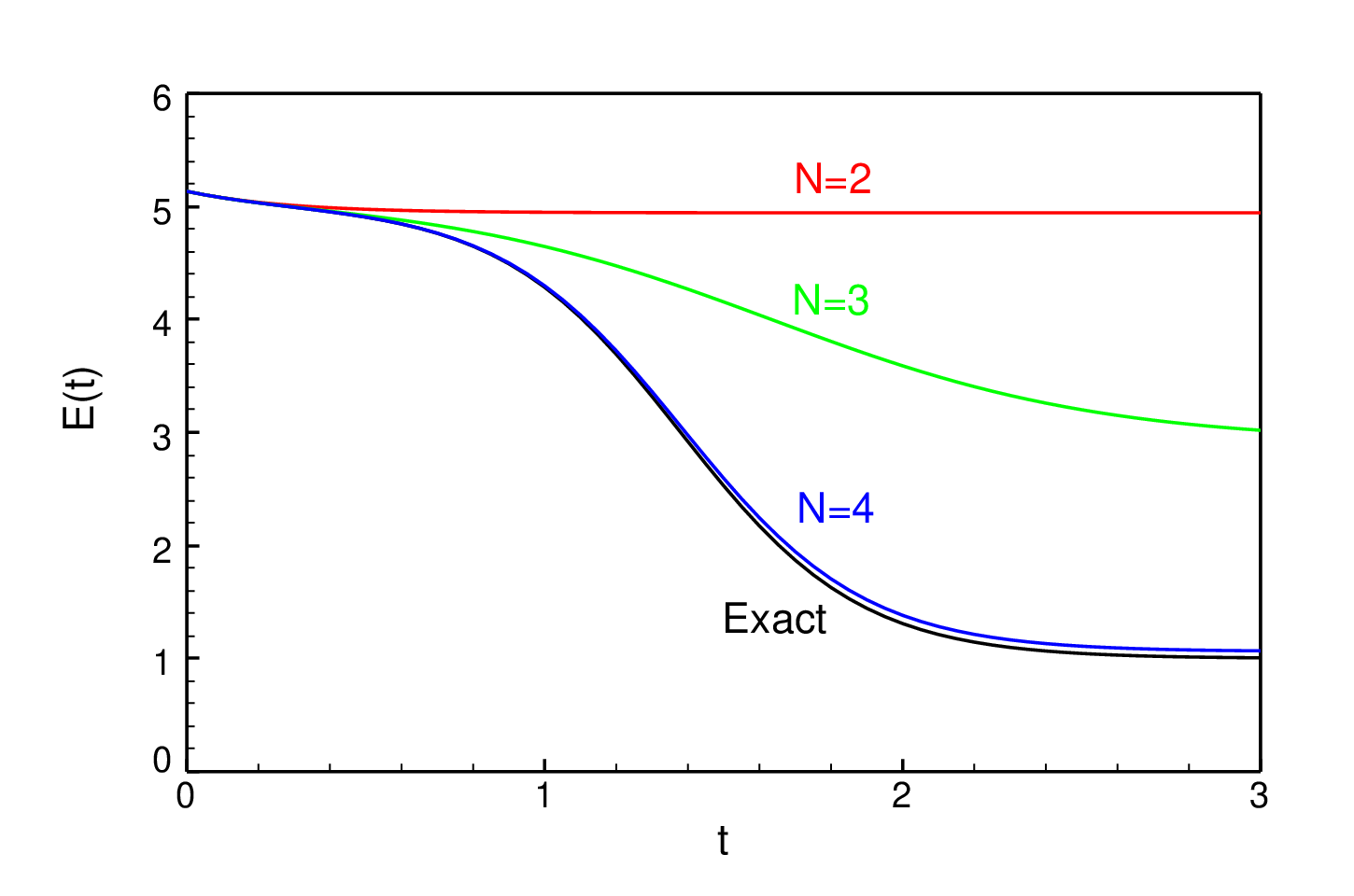
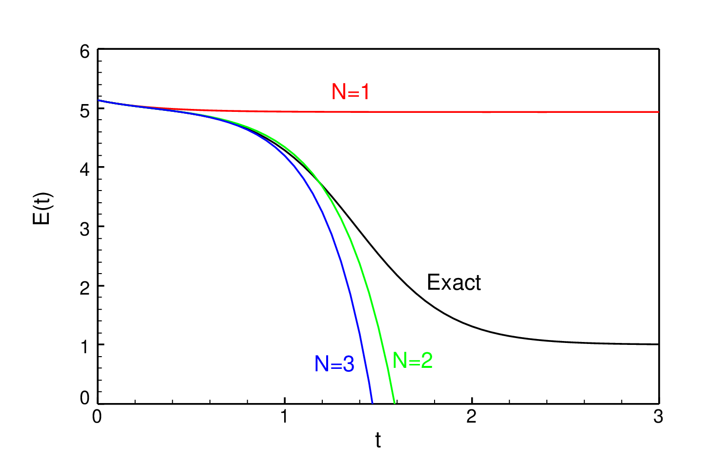
By means of the general results of the preceding section we can easily calculate the generating function $E(t)$ approximately in two ways: as $U^{(N)}(t)=-Z_{N}^{\prime}(t)/Z_{N}(t)$ from equation (13) and directly from equation (22). Fig 1 shows that $U^{(N)}(t)$ approaches the exact generating function $E(t)$ for all $0\leq t<\infty$ as $N$ increases. On the other hand, the approximate expression $E^{(N)}(t)$ given by Eq. (22) is an unsatisfactory approximation to the exact $E(t)$ as shown in Fig. 2 (except for sufficiently small values of $t$). This situation does not appear to improve as $N$ increases. It is found that $\lim_{t\rightarrow\infty}E^{(N)}(t)=-\infty$ for $N=2,3$ because in both cases there is one negative root $b_{j}$ associated to a negative coefficient $A_{j}$. For example, $A_{1}\approx-0.0170$, $A_{2}\approx 0.147$, $A_{3}\approx 0.000617$, $b_{1}\approx-3.87$, $b_{2}\approx 4.04$, and $b_{3}\approx 9.29$ for $N=3$. Note that the curves in both figures are directly comparable in the sense that the calculation of either $Z_{N+1}(t)$ and $E^{(N)}(t)$ requires exactly the same number of moments $\mu_{j}$ ($2N+1$). The behaviour of $E^{(N)}(t)$ for larger $N$ may be different; for example, for $N=4,5$ there are two negative roots and $\lim_{t\rightarrow\infty}E^{(N)}(t)=+\infty$.

The anomalous behaviour of $E^{(N)}(t)$ is due to the poles of $E(t)$ in the complex $t$–plane. Note that Eq. (28) exhibits three real poles in the $u$–plane and the closest to the origin is located at $u\approx-0.0040$. It is reasonable to assume that the CMX ansatz $E^{(N)}(t)$ should approach the Taylor series about $u=0$ for $E(t)$ when the approach is successful. However, this expansion does not converge for $u=1$ which is necessary for matching the $t$–expansion and exponential series at $t=0$. This problem was discussed by Amore et al[11] by means of two–level models and we see it here again for the harmonic oscillator. Those authors have shown that the CMX approximants for the harmonic oscillator with the trial function (27) converge towards the second–excited state $E_{2}=5$. From the approximate expressions $E^{(N)}(t)$ with $N=1,2,3$ we obtain $A_{0}\approx 4.932,5.015,5.002$, respectively, in agreement with those results. This example shows that the CMX approximants may converge to a meaningful result even when the ansatz $E^{(N)}(t)$ (on which the approach is based) is an unacceptable global approximation to $E(t)$.

Knowles[5] argued that if the connected moments $I_{k}$ are positive for all $k$ then the $b_{i}$ are real and positive. Later, Massano et al[6] and Mancini et al[7] suggested that Knowles’ argument may not be valid and that it is the Hadamard determinants constructed from the $I_{k}$ that should be positive. The example just analysed supports the latter conclusion because the first connected moments are all positive ($\approx 5.13$, $0.665$, $2.12$, $11.2$, $40.0$, $216$, $979$) but one of the roots is negative as shown above. We realize that the general formulas derived in Sec. II are most useful for this kind of analysis. In fact, the calculation of the roots $b_{j}$ by means of present formulas is almost as easy as the calculation of the Hadamard determinants and the former provide a much clearer indication of the suitability of the ansatz $E^{(N)}(t)$ as an approach for $E(t)$.

By means of the example discussed above we do not want to convey the wrong impression that the CMX is suitable for the calculation of excited–state energies because it is quite difficult to choose an appropriate trial function for this purpose (except when we can exploit the symmetry of the problem to make the trial function orthogonal to the ground–state[20]). The main interest in that exactly solvable problem is to show that we may predict an anomalous behaviour of the CMX by means of the roots $b_{j}$. If they are not real and positive it is reasonable to suspect that the trial function may not be suitable and that it is convenient to choose another one. For example, if $\phi(x)=e^{-x^{2}}$ all the roots $b_{j}$ are positive and the resulting $E^{(N)}(t)$ is a remarkably good approximation to $E(t)$ for all $0\leq t<\infty$ even at the low orders $N=1,2$.

Finally, we explore the possibility of calculating of the correlation function

$$C(t)=Z(it)=\left\langle\phi\right|e^{-it\hat{H}}\left|\phi\right\rangle$$

(29)

where $\left|\phi\right\rangle=\left|\phi(0)\right\rangle$ is the initial state normalized to unity and $\left|\phi(t)\right\rangle=e^{-it\hat{H}}\left|\phi(0)\right\rangle$ is the state at time $t$. In particular we concentrate on the real function $\left|C(t)\right|^{2}$.

As a first example we consider the harmonic oscillator (26) and the trial function

$$\phi(x)=\left(\frac{2}{\pi}\right)^{1/4}\mathbf{e}^{-x^{2}}$$

(30)

The exact correlation function is

$$\left|C(t)\right|^{2}=\frac{4\sqrt{2}}{\sqrt{41-9\cos{\left(4t\right)}}}$$

(31)

Fig. 3 shows results for $N=2,3,4,5$. There is no doubt that $\left|Z_{N}(it)\right|^{2}$ converges towards $\left|C(t)\right|^{2}$ as $N$ increases. The approximation is satisfactory within the first period but the errors accumulate as $t$ increases. This fact is not surprising because the approximate expression is constructed from the Maclaurin series for $Z(it)$.

The second example is the anharmonic oscillator

$$\hat{H}=-\frac{d^{2}}{dx^{2}}+x^{4}$$

(32)

and the same trial function (30). Fig. 4 shows that the approximate results for $N=2,3,4,5$ follow the same trend as in the case of the harmonic oscillator. At first sight it may be surprising that the convergence rate for the anharmonic oscillator appears to be greater than for the harmonic one. The reason is that the chosen trial state exhibits a greater overlap with the ground state of the former. Note that the magnitude of the coefficient $A_{0}$ of $Z_{N}(t)$ tells us that $\left|\left\langle\phi\right.\left|\psi_{0}\right\rangle\right|^{2}$ is approximately 0.943 for the harmonic oscillator and 0.981 for the anharmonic one.

As a two–dimensional example we consider the anharmonic oscillator

$$\hat{H}=-\frac{d^{2}}{dx^{2}}-\frac{d^{2}}{dy^{2}}+x^{2}+y^{2}+\lambda x^{2}y^{2}$$

(33)

where $\lambda>0$, and the trial function

$$\phi(x,y)=\left(\frac{2}{\pi}\right)^{1/2}e^{-x^{2}-y^{2}}$$

(34)

Fig. 5 shows results for $\lambda=0.5$ that look quite similar to those for the one–dimensional models.

One does not expect that it may be possible to construct $C(t)$ from its Taylor expansion about $t=0$ in all the cases. The problems discussed above are simple examples of single–well oscillators. In the case of the double–well oscillator $V(x)=(x^{2}-1)^{2}$ and the trial state localized in one of the wells $\phi(x)=\left(\frac{2}{\pi}\right)^{1/4}e^{-(x-1)^{2}}$ the approximants to $\left|C(t)\right|^{2}$ do not appear to converge although the results for $Z(t)$ look reasonable. If, on the other hand, we locate the initial state on top of the barier (for example, Eq. (30)) then the results are as accurate as those for the single wells.

The main goal of this paper is to show that Prony’s method provides the full solution of the CMX equations in a straightforward and simple way. We have outlined the connection between Prony’s method and the procedure developed recently by Amore and Fernández[12]. Although both approaches are equivalent and Prony’s one is known since long ago it seems that the pseudo–secular determinants obtained by Amore and Fernández are not available elsewhere.

In spite of the fact that the harmonic oscillator with the trial function (27) was chosen as an illustrative example in two earlier papers[11, 12] we think that present discussion based on the exact generating function (28) is clearer and provides more information about the behaviour of the CMX ansatz $E^{(N)}(t)$. In particular, we have shown that this simple problem clearly illustrates that Knowles’ conclusion about the sign of the connected moments[5] is not valid as argued before by Massano et al[6] and Mancini et al[7].

It is clear that the roots $b_{i}$ provide a clear indication of the success of the CMX and the method developed by Amore and Fernández[12], as well as Prony’s method, make their calculation straightforward. Both procedures may be applied to the calculation of the autocorrelation function for simple quantum–mechanical models. If the approach converges then one obtains a reasonable analytic expression for the autocorrelation function within the first period of oscillation.

References

- [1] D. Horn and M. Weinstein, Phys. Rev. D 30, 1256 (1984).
- [2] D. Horn, M. Karliner, and M. Weinstein, Phys. Rev. D 31, 2589 (1985).
- [3] J. Cioslowski, Phys. Rev. Lett. 58, 83 (1987).
- [4] C. Stubbins, Phys. Rev. D 38, 1942 (1988).
- [5] P. Knowles, Chem. Phys. Lett. 134, 512 (1987).
- [6] W. J. Massano, S. P. Bowen, and J. D. Mancini, Phys. Rev. A 39, 4301 (1989).
- [7] J. D. Mancini, J. D. Prie, and W. J. Massano, Phys. Rev. A 43, 1777 (1991).
- [8] J. D. Mancini, Y. Zhou, and P. F. Meier, Int. J. Quantum Chem. 50, 101 (1994).
- [9] J. D. Mancini, Y. Zhou, P. F. Meier, W. J. Massano, and J. D. Prie, Phys. Lett. A 185, 435 (1994).
- [10] J. D Mancini, R. K. Murawski, V Fessatidis, and S. P. Bowen, Phys. Rev. B 72, 214405 (6 pp.) (2005).
- [11] P. Amore, F. M. Fernández, and M. Rodriguez, J. Phys. A, (in the press), arXiv:1011.2260v1 [quant-ph].
- [12] P. Amore and F. M. Fernández, Solution to the Equations of the Moment Expansions, arXiv:1110.0782v1 [quant-ph]
- [13] F. M. Fernández, Int. J. Quantum Chem. 109, 717 (2009). arXiv:0807.1442 [math-ph]
- [14] I. Bartashevich, Int. J. Quantum Chem. 108, 272 (2008).
- [15] R. Prony, Journal de l’École Polytechnique Floréal et Plairial, an III 1, 24 (1795).
- [16] L. Weiss and R. N. AcDnonough, SIAM Review 5, 145 (1963).
- [17] F. B. Hildebrand, Introduction to Numerical Analysis, Second ed. (Dover, New York, 1974).
- [18] J. Fuite, R. E. Marsh, and J. A. Tuszynski, Commun. Comput. Phys. 2, 87 (2007).
- [19] K. Holmström and J. Petersson, App. Math. Comput. 126, 31 (2002).
- [20] P. Amore and F. M. Fernández, Phys. Scr. 80, 055002 (5pp) (2009).