跳到论文正文
W Papers独立论文阅读器 arXiv:1111.3723 论文正文 计算阅读时间 · 0%
引用这篇论文根据当前论文元数据生成,正式投稿前建议核对。


License: arXiv.org perpetual non-exclusive license
arXiv:1111.3723v4 [hep-th] 07 Nov 2012

OCU-PHYS 359

November, 2011

Proving the Absence of the Perturbative

Corrections to the 𝒩=2\mathcal{N}=2 U⁡(1)U(1) Kähler Potential

Using the 𝒩=1\mathcal{N}=1 Supergraph Techniques

Sho Deguchia11 1 e-mail: deguchi@sci.osaka-cu.ac.jp

a Department of Mathematics and Physics, Graduate School of Science
Osaka City University

3-3-138, Sugimoto, Sumiyoshi-ku, Osaka, 558-8585, Japan

Abstract

Perturbative 𝒩=2\mathcal{N}=2 non-renormalization theorem states that there is no perturbative correction to the Kähler potential ∫d4​θ​K​(Φ,Φ¯)\int d^{4}\theta K\left(\Phi,{\overline{\Phi}}\right). We prove this statement by using the 𝒩=1\mathcal{N}=1 supergraph techniques. We consider the 𝒩=2\mathcal{N}=2 supersymmetric U⁡(1)U(1) gauge theory which possesses general prepotential ℱ⁡(Ψ){\mathcal{F}}(\Psi).

1 Introduction

In quantum field theory, there are, in general, many loop corrections to the effective action. In the supersymmetric perturbative theory, there is non-renormalization theorem states that the corrections to the effective action take the form[1, 2, 3]

∫d4​𝒩θ∫d4x1⋯d4xnF1(x1,θ,θ¯)⋯Fn(xn,θ,θ¯)G(x1,⋯,xn),\displaystyle\int d^{4\mathcal{N}}\theta\int d^{4}x_{1}\cdots d^{4}x_{n}F_{1}(x_{1},\theta,{\overline{\theta}})\cdots F_{n}(x_{n},\theta,{\overline{\theta}})G(x_{1},\cdots,x_{n})~, (1)

where the function GG is translationally invariant and FF’s are product of superfields and their derivatives. There are no factors of □−1(=[∂m∂m]−1)\square^{-1}(=[\partial^{m}\partial_{m}]^{-1}) in the FF’s, so the d4​𝒩​θd^{4\mathcal{N}}\theta integration cannot be converted into a d2​𝒩​θd^{2\mathcal{N}}\theta integration without generating additional spacetime derivatives. In 𝒩=1\mathcal{N}=1 supersymmetric theory, there is no loop correction to the effective superpotential ∫d2​θ​f​(Φ)\int d^{2}\theta f(\Phi), while there is, in general, loop correction to the effective Kähler potential ∫d4​θ​Keff​(Φ,Φ¯)\int d^{4}\theta K_{\textrm{eff}}(\Phi,{\overline{\Phi}}). On the other hand, in 𝒩=2\mathcal{N}=2 supersymmetric U⁡(1)U(1) gauge theory, all of the loop corrections to the effective Kähler potential however cancel. This is because of that the action of 𝒩=2\mathcal{N}=2 supersymmetric theory takes the form of chiral (∫d2θ1d2θ2⋯\int d^{2}\theta_{1}d^{2}\theta_{2}\cdots). So there is no perturbative correction to the original terms of the action according to 𝒩=2\mathcal{N}=2 non-renormalization theorem [2, 3]. The 𝒩=2\mathcal{N}=2 non-renormalization theorem is given by using the unconstrained superfield [2, 4] VI​JV^{IJ}(=V¯I​J={\overline{V}}^{IJ}) as

Ψ∼D¯I​J​D¯I​J​DK​L​VK​L,\displaystyle\Psi\sim{\overline{D}}^{IJ}{\overline{D}}_{IJ}D_{KL}V^{KL}~, (2)

where I,J,K,LI,J,K,L are global S​U​(2)SU(2) indices, and this superfield satisfies the chirality condition and reality condition as follows [5].

DαI​Ψ=0,DI​J​Ψ=D¯I​J​Ψ¯.\displaystyle D^{I}_{\alpha}\Psi=0~,~~~D^{IJ}\Psi={\overline{D}}^{IJ}{\overline{\Psi}}. (3)

These conditions reduce the unwanted degree of freedom for the vector superfield. On the other hand, it is not known how this theorem is proven by using the 𝒩=1\mathcal{N}=1 formalism, where Ψ\Psi is represented as

Ψ⁡(y~,θ,θ~)=Φ⁡(y~,θ)+i​2​θ~α​𝒲α​(y~,θ)+θ~​θ~​∫d2​θ¯​Φ¯​(y~−i​θ~​σ​θ¯~,θ¯).\displaystyle\Psi(\tilde{y},\theta,\tilde{\theta})=\Phi(\tilde{y},\theta)+i\sqrt{2}\tilde{\theta}^{\alpha}{\mathcal{W}}_{\alpha}(\tilde{y},\theta)+\tilde{\theta}\tilde{\theta}\int d^{2}{\overline{\theta}}~\overline{\Phi}(\tilde{y}-i\tilde{\theta}\sigma\tilde{{\overline{\theta}}},{\overline{\theta}})~. (4)

where y~=x+i​θ​σ​θ¯+i​θ~​σ​θ~¯\tilde{y}=x+i\theta\sigma{\overline{\theta}}+i\tilde{\theta}\sigma{\overline{\tilde{\theta}}}, and θ~\tilde{\theta} is a second grassmann spinor. In this paper, we prove the cancellation of loop corrections to the effective Kähler potential. In contrast to the simple model we considered in paper, there are many calculations of one- and two-loop effective Kähler potential in general 𝒩=1\mathcal{N}=1 supersymmetric theories, which are performed in Ref. [6, 7, 8].

Outline of this paper is as follows. In Sec.2, we represent 𝒩=2\mathcal{N}=2 supersymmetric U⁡(1)U(1) gauge theory by using the 𝒩=1\mathcal{N}=1 formalism. In Sec.3, we construct super-Feynman rules and illustrate the correspondence between the supergraphs and the formulas by using an example. Sec.4 is the central part in this paper, where we prove the cancellation upto the nn-loop supergraphs.

2 𝒩=2\mathcal{N}=2 supersymmetric U⁡(1)U(1) gauge theory in the 𝒩=1\mathcal{N}=1 formalism

We consider a theory, which can be represented by using 𝒩=2\mathcal{N}=2 formalism as in Ref. [9]:

S⁡[Ψ,Ψ¯]=Im​∫d4​x​d2​θ​d2​θ~​ℱ​(Ψ),\displaystyle S[\Psi,{\overline{\Psi}}]={\textrm{Im}}\int d^{4}xd^{2}\theta d^{2}\tilde{\theta}~{\mathcal{F}}(\Psi)~, (5)

where ℱ{\mathcal{F}} is a polynomial and we postulate that the imaginary part of the second derivative ℱ{\mathcal{F}} is positive:

ℱ⁡(x)=∑k=2nak​xkk!,ai∈ℂ,n⩾2.\displaystyle{\mathcal{F}}(x)=\sum_{k=2}^{n}\frac{a_{k}x^{k}}{k!},~~~a_{i}\in\mathbb{C},~~n\geqslant 2~. (6)

In the 𝒩=1\mathcal{N}=1 SUSY formalism, the action is rewritten as:

S⁡[Φ,Φ¯,V]=Im​∫d8​z​Φ¯​∂ℱ⁡(Φ)∂Φ+Im​∫d6​z​12!​∂2ℱ⁡(Φ)∂Φ​∂Φ​𝒲α​𝒲α.\displaystyle S[\Phi,{\overline{\Phi}},V]={\textrm{Im}}\int d^{8}z~{\overline{\Phi}}\frac{\partial{\mathcal{F}}(\Phi)}{\partial\Phi}+{\textrm{Im}}\int d^{6}z\frac{1}{2!}\frac{\partial^{2}{\mathcal{F}}(\Phi)}{\partial\Phi\partial\Phi}{\mathcal{W}}^{\alpha}{\mathcal{W}}_{\alpha}. (7)

To obtain the effective Kähler potential ∫d4​θ​Keff​(ϕ,ϕ¯)\int d^{4}\theta~K_{\textrm{eff}}(\phi,{\overline{\phi}}) we decompose chiral superfield Φ\Phi into classical part ϕ\phi and perturbative part Φ\Phi, and perform the path integral respect to Φ\Phi and VV as follows.

exp⁡(i​∫d8​z​Keff​(ϕ,ϕ¯))=∫[𝑑Φ]​[𝑑Φ¯]​[𝑑V]​exp⁡(i​S​[ϕ+Φ,ϕ¯+Φ¯,V]),\displaystyle\exp\left(i\int d^{8}z~K_{\textrm{eff}}(\phi,{\overline{\phi}})\right)=\int[d\Phi][d{\overline{\Phi}}][dV]\exp\left(iS[\phi+\Phi,{\overline{\phi}}+{\overline{\Phi}},V]\right), (8)
S⁡[ϕ+Φ,ϕ¯+Φ¯,V]=Im​∫d8​z​∑k=2nℱ(k)​(ϕ)k!​{Φ¯​Φk−1+12!​Φk−2​(Dα​V)​(−14​D¯2​Dα​V)},\displaystyle S\left[\phi+\Phi,{\overline{\phi}}+{\overline{\Phi}},V\right]={\textrm{Im}}\int~d^{8}z\sum_{k=2}^{n}\frac{{\mathcal{F}}^{(k)}(\phi)}{k!}\left\{{\overline{\Phi}}\Phi^{k-1}+\frac{1}{2!}\Phi^{k-2}\left(D^{\alpha}V\right)\left(-\frac{1}{4}{\overline{D}}^{2}D_{\alpha}V\right)\right\}~, (9)

where we do not consider the derivatives of ϕ\phi as in Ref.[8], because we focus only on the effective Kähler potential.

3 Super-Feynman Rules

In this section, we explain super-Feynman rules needed for deriving the effective action. We use the super-Feynman rules introduced by Grisaru, Roc̆ek, and Siegel[1].

  1. I)

    For each line,

    chiral line:[Uncaptioned image]=\displaystyle\textrm{chiral line}:~~~\raisebox{-0.43057pt}{\includegraphics[scale={0.7}]{ppb.eps}}~~~= ig⁡(ϕ,ϕ¯)​□​δ8​(z1−z2)=⟨Φ⁡(z1)​Φ¯​(z2)⟩GRS,\displaystyle~~~\frac{i}{g(\phi,{\overline{\phi}})\square}\delta^{8}(z_{1}-z_{2})~~~=~~~\langle\Phi(z_{1}){\overline{\Phi}}(z_{2})\rangle_{\textrm{GRS}}, (10)
    vector line:[Uncaptioned image]=\displaystyle\textrm{vector line}:~~~\raisebox{0.0pt}{\includegraphics[scale={0.7}]{vv.eps}}~~~= −i2​g​(ϕ,ϕ¯)​□​δ8​(z1−z2)=⟨V⁡(z1)​V​(z2)⟩,\displaystyle~~~\frac{-i}{2g(\phi,{\overline{\phi}})\square}\delta^{8}(z_{1}-z_{2})~~~=~~~\langle V(z_{1})V(z_{2})\rangle, (11)

    where g⁡(ϕ,ϕ¯)≡Im​(ℱ′′​(ϕ))g(\phi,{\overline{\phi}})\equiv{\textrm{Im}}({\mathcal{F}}^{\prime\prime}(\phi)) and □≡∂m∂m\square\equiv\partial^{m}\partial_{m}.

  2. II)

    For each nn-point vertex (n⩾3n\geqslant 3),

    [Uncaptioned image]=\displaystyle\raisebox{-17.22217pt}{\includegraphics[scale={0.6}]{holo_vertices.eps}}~~~~~= ∫d8​z​12​ℱ(n)​(ϕ),\displaystyle~~~~~\int d^{8}z~\frac{1}{2}{\mathcal{F}}^{(n)}(\phi)~~, (12)
    [Uncaptioned image]=\displaystyle\raisebox{-17.22217pt}{\includegraphics[scale={0.6}]{holo_vertices_anti.eps}}~~~~~= ∫d8​z​(−12​ℱ¯(n)​(ϕ¯)),\displaystyle~~~~~\int d^{8}z~(-\frac{1}{2}{\overline{{\mathcal{F}}}}^{(n)}({\overline{\phi}}))~~, (13)

    where ℱ(n)​(ϕ)=∂n∂ϕn​ℱ​(ϕ){\mathcal{F}}^{(n)}(\phi)=\frac{\partial^{n}}{\partial\phi^{n}}{\mathcal{F}}(\phi).

  3. III)

    At each outgoing (or incoming) chiral line, we act −14​D2-\tfrac{1}{4}D^{2} (or −14​D¯2-\tfrac{1}{4}{\overline{D}}^{2}).

  4. IV)

    At each set of two vector lines connected with the holomorphic vertices, we act −14​D¯2​Dα-\tfrac{1}{4}{\overline{D}}^{2}D^{\alpha} and DαD_{\alpha}. At each set of two vector lines connected with the anti-holomorphic vertices, we act −14​D2​D¯α˙-\tfrac{1}{4}D^{2}{\overline{D}}_{\dot{\alpha}} and D¯α˙{\overline{D}}^{\dot{\alpha}}.

  5. V)

    (−)(-) sign is multiplied per one vector loop. This is because of anti-commutativity of operators acting at the vector lines in Rule IV.

  6. VI)

    Each supergraph is multiplied by symmetric factor.

3.1 Supergraph/Formula correspondence

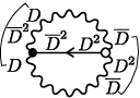
Here we consider a correspondence between the formulas and the supergraphs. The following vacuum amplitude corresponds to the supergraph as in Fig.1.

⟨∫dz18(12ℱ(3)(ϕ1))12!Φ1(D1αV1)(−14D¯12D1​αV1)\displaystyle\left\langle\int dz_{1}^{8}~(\frac{1}{2}{\mathcal{F}}^{(3)}(\phi_{1}))\frac{1}{2!}\Phi_{1}(D_{1}^{\alpha}V_{1})(-\frac{1}{4}{\overline{D}}_{1}^{2}D_{1\alpha}V_{1})\right.
⋅∫dz28(−12ℱ¯(3)(ϕ¯2))12!Φ¯2(D¯2​α˙V2)(−14D2D¯2α˙V2)⟩connected\displaystyle~~~~~~~\cdot\left.\int dz_{2}^{8}~(-\frac{1}{2}{\overline{{\mathcal{F}}}}^{(3)}({\overline{\phi}}_{2}))\frac{1}{2!}{\overline{\Phi}}_{2}({\overline{D}}_{2{\dot{\alpha}}}V_{2})(-\frac{1}{4}D^{2}{\overline{D}}_{2}^{{\dot{\alpha}}}V_{2})\right\rangle_{\textrm{connected}} (14)
=(−)​12!​∫d​z18​∫d​z28​(12​ℱ(3)​(ϕ1))​(−12​ℱ¯(3)​(ϕ¯2))\displaystyle=(-)\frac{1}{2!}\int dz_{1}^{8}\int dz_{2}^{8}(\frac{1}{2}{\mathcal{F}}^{(3)}(\phi_{1}))(-\frac{1}{2}{\overline{{\mathcal{F}}}}^{(3)}({\overline{\phi}}_{2}))
⋅((−14​D¯12)​(−14​D22)​⟨Φ1​Φ¯2⟩GRS)​((−14​D¯12​D1​α)​(D¯2​α˙)​⟨V1​V2⟩)\displaystyle~~~~~~~\cdot\left((-\frac{1}{4}{\overline{D}}_{1}^{2})(-\frac{1}{4}D_{2}^{2})\left\langle\Phi_{1}{\overline{\Phi}}_{2}\right\rangle_{\textrm{GRS}}\right)\left((-\frac{1}{4}{\overline{D}}_{1}^{2}D_{1\alpha})({\overline{D}}_{2{\dot{\alpha}}})\langle V_{1}V_{2}\rangle\right)
⋅((−14​D2​D¯2α˙)​(D1α)​⟨V2​V1⟩)\displaystyle~~~~~~~\cdot\left((-\frac{1}{4}D^{2}{\overline{D}}_{2}^{{\dot{\alpha}}})(D_{1}^{\alpha})\langle V_{2}V_{1}\rangle\right) (15)
=(−)​12!​∫d​z18​∫d​z28​(12​ℱ(3)​(ϕ1))​(−12​ℱ¯(3)​(ϕ¯2))\displaystyle=(-)\frac{1}{2!}\int dz_{1}^{8}\int dz_{2}^{8}(\frac{1}{2}{\mathcal{F}}^{(3)}(\phi_{1}))(-\frac{1}{2}{\overline{{\mathcal{F}}}}^{(3)}({\overline{\phi}}_{2}))
⋅((−14​D2)​(−14​D¯2)​ig​□​δ8​(z1−z2))​((−14​D¯12​D1​α)​(D¯2​α˙)​−i2​g​□​δ8​(z1−z2))\displaystyle~~~~~~~\cdot\left((-\frac{1}{4}D^{2})(-\frac{1}{4}{\overline{D}}^{2})\frac{i}{g\square}\delta^{8}(z_{1}-z_{2})\right)\left((-\frac{1}{4}{\overline{D}}_{1}^{2}D_{1\alpha})({\overline{D}}_{2{\dot{\alpha}}})\frac{-i}{2g\square}\delta^{8}(z_{1}-z_{2})\right)
⋅((−14​D2​D¯2α˙)​(D1α)​−i2​g​□​δ8​(z1−z2)),\displaystyle~~~~~~~\cdot\left((-\frac{1}{4}D^{2}{\overline{D}}_{2}^{{\dot{\alpha}}})(D_{1}^{\alpha})\frac{-i}{2g\square}\delta^{8}(z_{1}-z_{2})\right), (16)

where the over all minus sign comes from the existence of one vector loop. The front coefficients 12!\frac{1}{2!} are symmetric factors come from exchanging of the vector superfield lines.
Refer to caption
Figure 1: one of the 2-loop supergraphs. (Lines connecting operators denote the pairs of the spinor contractions)

4 Cancellation of supergraphs

In this section, we prove the cancellation of loop corrections to the effective Kähler potential K⁡(Φ,Φ¯)K(\Phi,{\overline{\Phi}}). Cancellation of the lowest order correction is proven in Sec.4.1. Cancellation of the holomorphic loops is proven in Sec.4.2. For simplicity, the vertices are redefined as the summation of the contracted holomorphic trees as described in Sec.4.3, and it is given how operators act typically in chiral line and vector line except common operators in Sec.4.4. To begin with cancellation of 2-loops is proven in Sec.4.5. Final Sec.4.6 is the essence of our paper where we prove that all of the nn-loop corrections to the effective Kähler potential cancel.

4.1 1-loop

Quadratic term of the action include the superfields called: chiral superfields Φ\Phi,Φ¯{\overline{\Phi}}, vector superfield VV, Faddev-Pappov ghosts CC,C′C^{\prime},C¯{\overline{C}},C′¯{\overline{C^{\prime}}}, and Nielsen-Kallosh ghost χ\chi,χ¯{\overline{\chi}} as follow.

Squad=∫d8​z​(g​Φ​Φ¯+g​V​□​V−C′​C¯−C′¯​C−2​g​χ¯​χ),S_{\textrm{quad}}=\int d^{8}z\left(g\Phi{\overline{\Phi}}+gV\square V-C^{\prime}{\overline{C}}-{\overline{C^{\prime}}}C-2g{\overline{\chi}}\chi\right),

where g=Im​ℱ(2)​(ϕ)g={\textrm{Im}}{\mathcal{F}}^{(2)}(\phi). Lowest-order correction takes the form:

zquad=∫[𝑑Φ]​[𝑑Φ¯]​[𝑑V]​[𝑑C]​[𝑑C¯]​[d​C′]​[𝑑C′¯]​[𝑑χ]​[𝑑χ¯]​exp⁡(i​Squad).z_{\textrm{quad}}=\int[d\Phi][d{\overline{\Phi}}][dV][dC][d{\overline{C}}][dC^{\prime}][d{\overline{C^{\prime}}}][d\chi][d{\overline{\chi}}]\exp(iS_{\textrm{quad}}).

In this case, vector term do not depend on gg as follow.

∫[𝑑V]​exp⁡(∫d8​z​[g​V​□​V+ε​V​□​V])=∫[𝑑V]​exp⁡(∫d8​z​[g​V​□​V]).\int[dV]\exp\left(\int d^{8}z~[gV\square V+\varepsilon V\square V]\right)=\int[dV]\exp\left(\int d^{8}z~[gV\square V]\right).

This is because of that ε\varepsilon-vertex do not have operators like DD and D¯{\overline{D}}. So perturbative calculation derive the delta function δ2​(θ−θ)​δ2​(θ¯−θ¯)=0\delta^{2}(\theta-\theta)\delta^{2}({\overline{\theta}}-{\overline{\theta}})=0. Chiral term cancel with term of Nielsen-Kallosh ghost which is fermionic, and Faddev-Poppov ghost term do not depends on g⁡(ϕ,ϕ¯)g(\phi,{\overline{\phi}}). Lowest-order correction is absent.

4.2 Holomorphic loop

Here we mean by holomorphic loop a loop constructed only with holomorphic vertices. The holomorphic loops cancel each other by the following summation.
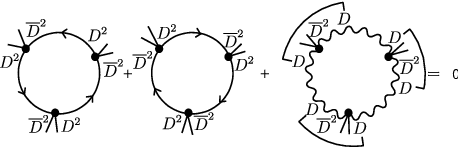
Refer to caption
Figure 2: holomorphic loop cancelation

We confirm the Fig.2 by partial integrations respect to DD and D¯{\overline{D}} in the following procedure.

Summation of first two supergraphs in Fig.2 gives the following amplitude, here we omit the common factors(D¯2{\overline{D}}^{2} and ∼□−1\sim\square^{-1}) between the chiral loops and the vector loop.

2⋅(−14​D2​δ8)​(−14​D2​δ8)​(−14​D2​δ8)2\cdot(-\frac{1}{4}D^{2}~\delta^{8})(-\frac{1}{4}D^{2}~\delta^{8})(-\frac{1}{4}D^{2}~\delta^{8})

Third supergraph gives

(−)⋅(−)3​(−12)3⋅(Dα​Dβ​δ8)​(Dβ​Dγ​δ8)​(Dγ​Dα​δ8)\displaystyle(-)\cdot(-)^{3}(-\frac{1}{2})^{3}\cdot(D_{\alpha}D^{\beta}~\delta^{8})(D_{\beta}D^{\gamma}~\delta^{8})(D_{\gamma}D^{\alpha}~\delta^{8})
=(−)⋅(−)3​(−12)3⋅(−12​δαβ​D2​δ8)​(−12​δβγ​D2​δ8)​(−12​δγα​D2​δ8)\displaystyle~~~~~=(-)\cdot(-)^{3}(-\frac{1}{2})^{3}\cdot(-\frac{1}{2}\delta_{\alpha}^{\beta}D^{2}~\delta^{8})(-\frac{1}{2}\delta_{\beta}^{\gamma}D^{2}~\delta^{8})(-\frac{1}{2}\delta_{\gamma}^{\alpha}D^{2}~\delta^{8})
=(−)​2⋅(−14​D2​δ8)​(−14​D2​δ8)​(−14​D2​δ8),\displaystyle~~~~~=(-)2\cdot(-\frac{1}{4}D^{2}~\delta^{8})(-\frac{1}{4}D^{2}~\delta^{8})(-\frac{1}{4}D^{2}~\delta^{8}),

where (−)3(-)^{3} comes from change of variables zz to z′z^{\prime}, (−12)3(-\frac{1}{2})^{3} is ratio between propagators of chiral superfields and vector superfields, and we have used Dα​Dβ=−12​δαβ​D2D_{\alpha}D^{\beta}=-\frac{1}{2}\delta_{\alpha}^{\beta}D^{2}.

4.3 Contractions of the holomorphic trees

Any chiral line connecting two holomorphic vertices is eliminated by integrating out the delta function δ8​(z−z′)\delta^{8}(z-z^{\prime}) on the lines as in Fig.3. Typically the delta functions at these chiral lines take the form:

(−14​D2)​(−14​D¯2)​(ig​□)​δ8.(-\frac{1}{4}D^{2})(-\frac{1}{4}{\overline{D}}^{2})(\frac{i}{g\square})\delta^{8}.

By partial integral respect to −14​D2-\frac{1}{4}D^{2} from the another line, we can act the additional operator to this chiral line as follow.

(−14​D2)​(−14​D¯2)​(−14​D2)​(ig​□)​δ8=−(−14​D2)​(ig)​δ8.\displaystyle(-\frac{1}{4}D^{2})(-\frac{1}{4}{\overline{D}}^{2})(-\frac{1}{4}D^{2})(\frac{i}{g\square})\delta^{8}=-(-\frac{1}{4}D^{2})(\frac{i}{g})\delta^{8}. (17)

Finally −14​D2-\frac{1}{4}D^{2} is back to the initial line by partial integral. So we can integrate out the delta functions of inner lines.

Refer to caption
Figure 3: Chiral tree contraction

On the other hand, any vector line connecting two holomorphic vertices is eliminated as in Fig.4 in the same way. Typically the delta functions at these vector lines take the form:

(−)​(Dα)​(Dβ​(−14​D¯2))​(−i2​g​□)​δ8.(-)(D_{\alpha})(D^{\beta}(-\frac{1}{4}{\overline{D}}^{2}))(\frac{-i}{2g\square})\delta^{8}.

By partial integral, −14​D2-\frac{1}{4}D^{2} acts as follows.

→(−)​(−14​D¯2)​(Dα)​(Dβ​(−14​D¯2))​(−i2​g​□)​δ8\displaystyle\rightarrow(-)(-\frac{1}{4}{\overline{D}}^{2})(D_{\alpha})(D^{\beta}(-\frac{1}{4}{\overline{D}}^{2}))(\frac{-i}{2g\square})\delta^{8} (18)
=(−)​(−14​D¯2)​(−12​δαβ​D2)​(−14​D¯2)​(−i2​g​□)​δ8\displaystyle=(-)(-\frac{1}{4}{\overline{D}}^{2})(-\frac{1}{2}\delta_{\alpha}^{\beta}D^{2})(-\frac{1}{4}{\overline{D}}^{2})(\frac{-i}{2g\square})\delta^{8} (19)
=(−14​D¯2)​(−14​D2)​(−14​D¯2)​(ig​□)​δ8\displaystyle=(-\frac{1}{4}{\overline{D}}^{2})(-\frac{1}{4}D^{2})(-\frac{1}{4}{\overline{D}}^{2})(\frac{i}{g\square})\delta^{8} (20)
=(−14​D¯2)​(−□)​(ig​□)​δ8\displaystyle=(-\frac{1}{4}{\overline{D}}^{2})(-\square)(\frac{i}{g\square})\delta^{8} (21)
→−ig​δ8.\displaystyle\rightarrow-\frac{i}{g}\delta^{8}. (22)
Refer to caption
Figure 4: vector tree contraction

In this way we obtain vertices made from the contracted holomorphic trees as in Fig.5, and we use these vertices as fundamental ones. Then the additional super-Feynman rule arise, that the holomorphic and anti-holomorphic vertices can not connect with the holomorphic and anti-holomorphic ones, respectively. This rule prevents the overlap of summation of trees.

Refer to caption
Figure 5: These vertices are made from the contracted holomorphic trees

4.4 Differences between chiral lines and vector lines

As our purpose in this paper is seeing the cancellation between the loop corrections, we focus on the differences between chiral lines and vector lines. There are two types of nn-point vertices that include two vector line and that include only chiral lines. But these coefficients are the same. However, ways of acting momentum operator Pm=i∂mP_{m}=i\partial_{m} are different. Difference between chiral lines and vector lines are following.

Each vertex including only chiral lines have one opposite directional chiral line. After little calculation like in Sec.4.2, we can see that P2P^{2} act at these opposite directional chiral lines as in Fig.6, where we omitted operators which are common to chiral lines and vector lines.

Refer to caption
Figure 6: typical way of how operators act at vertices including only chiral lines.

Each vertex including vector lines is connected with two vector lines. In the same way, we can see that P̸{\not}P act at these vector lines as in Fig.7, where minus sign comes from existence of one vector line loop (See Sec.3) and we omitted operators which are common to chiral lines and vector lines. (Slashed vector operators, for example, A̸{\not}A denote Am​σmA_{m}\sigma^{m} or Am​σ¯mA_{m}{\overline{\sigma}}^{m}. A̸B̸C̸⋯{\not}A{\not}B{\not}C\cdots denote the product of alternate σm\sigma^{m}’s and σ¯m{\overline{\sigma}}^{m}’s as (AmBnCk⋯)(σmσ¯nσk⋯)(A_{m}B_{n}C_{k}\cdots)(\sigma^{m}{\overline{\sigma}}^{n}\sigma^{k}\cdots).)

Refer to caption
Figure 7: typical way of how operators act at vertices including vector lines. (vector line is always closed. See Sec.3)

4.5 2-loop

Holomorphic loop diagrams cancel as discussed in Sec.4.2. Similarly, non-holomorphic loop diagrams cancel. In this subsection, we consider the two loop diagrams as in Fig.8. There are other diagrams including tadpole. However we do not consider these diagrams in this subsection. In Sec.4.6, we show the cancellation, including the tadpoles. The cancellation of these two diagrams is shown by partial integral respect to PmP_{m} —(Here, we used P2=12​Tr​(P̸​P̸)=12​Pm​Pn​Tr​(σm​σ¯n)P^{2}=\frac{1}{2}{\textrm{Tr}}({\not}P{\not}P)=\frac{1}{2}P_{m}P_{n}{\textrm{Tr}}(\sigma^{m}{\overline{\sigma}}^{n})).

Refer to caption
Figure 8: 2-loop graphs

4.6 nn-loop

Difference between chiral lines and vector lines is summarized in Sec.4.4. Then we show that difference is mostly only the way of how operator P̸{\not}P are acting. In this way, we now focus on a supergraph including only chiral lines as left hand side in Fig.9. This supergraph can be transformed into supergraphs including vector like lines as right hand side in Fig.9 by appropriate partial integral respect to P̸{\not}P. Then we notice that these supergraphs cancel for opposite sign.

Refer to caption
Figure 9: transformation of supergraph from one including only chiral lines to other including vector lines.

The transformations from chiral lines to vector like lines are given by appropriate partial integral respect to P̸{\not}P as follow.

P12P32⋯=12Tr(P̸12P̸32⋯)⟶12Tr(P̸1P̸2P̸3P̸4⋯),\displaystyle P_{1}^{2}P_{3}^{2}\cdots=\tfrac{1}{2}{\textrm{Tr}}({\not}P^{2}_{1}{\not}P^{2}_{3}\cdots)\longrightarrow\tfrac{1}{2}{\textrm{Tr}}({\not}P_{1}{\not}P_{2}{\not}P_{3}{\not}P_{4}\cdots), (23)

where subscript 1,2,⋯1,2,\cdots denote position z1,z2,⋯z_{1},z_{2},\cdots, and we used P2​12×2=P̸2P^{2}1_{2\times 2}={\not}P^{2}. We can describe above state by using supergraphs as in Fig.10. Here we are focusing on only one route of partial integral for simplicity, so we in fact need to consider about another routes by choosing another lines for acting P̸{\not}P.

Refer to caption
Figure 10: transform chiral line to vector like line by partial integral respect to P̸{\not}P.

However this procedure will comes to two types of dead ends that there is no next P2P^{2} to do the partial integration as in Fig.11 and Fig.12, respectively.

Refer to caption
Figure 11: dead ends type 1
Refer to caption
Figure 12: dead ends type 2

In the dead ends type 1 as in Fig.11, we can split the trace by considering opposite directional chiral loop as in Fig.13, where we use the identity:

(A̸1A̸2⋯A̸2​n)+(A̸2​n⋯A̸2A̸1)=2Tr(A̸1A̸2⋯A̸2​n)12×2.\displaystyle({\not}A_{1}{\not}A_{2}\cdots{\not}A_{2n})+({\not}A_{2n}\cdots{\not}A_{2}{\not}A_{1})~=~2{\textrm{Tr}}({\not}A_{1}{\not}A_{2}\cdots{\not}A_{2n})1_{2\times 2}. (24)
Refer to caption
Figure 13: split the trace

And so we can continue the procedure by turning P̸{\not}P into another line.

In the dead ends type 2 as in Fig.12, the partial integral procedure hits into the vector like loop previously transformed by appropriate partial integrations. But these partial integral routes cancel with the other routes as in Fig.14. Thus we can neglect these hitting routes, and continue the partial integral procedure.

Refer to caption
Figure 14: hitting routes cancel.

Ultimately partial integral procedure back to start point. Then many supergraphs including vector like loops are generated. However there is a situation that we can not generate all of the supergraphs including vector line by doing the single above procedure. This is because of that, in the single procedure, we consider the partial integral along the one side direction of chiral line or this opposite direction. So there are regions that we can not reach by the single partial integral as in Fig.15.

Refer to caption
Figure 15: G+G+ is a region of the supergraphs that we can reach along the lines with the direction of chiral line. On the other hand, G−G- is a region of the supergraphs that we can reach along the lines with the opposite direction to the direction of chiral line.

But we can cover all supergraphs including vector lines by executing the above procedure repeatedly from the different regions and by flipping the direction of partial integral procedure for the direction of chiral lines.

Then all of the supergraphs including vector superfield are generated with opposite sign, so all of the supergraphs cancel, including tadpoles.

5 Conclusion and Outlook

We have proven that all of the loop corrections to the effective Kähler potential, in 𝒩=2\mathcal{N}=2 U⁡(1)U(1) gauge theory, cancel each other by using 𝒩=1\mathcal{N}=1 supergraph techniques instead of 𝒩=2\mathcal{N}=2 ones.

As for applications, the extension to the U​(1)NU(1)^{N} case is rather trivially carried out while the extension to the U⁡(N)U(N) case requires more efforts. On the other hand, 𝒩=2\mathcal{N}=2 supersymmetry is broken in nature and there is U⁡(N)U(N) gauge theory in which 𝒩=2\mathcal{N}=2 supersymmetry is partially and spontaneously broken [11, 12, 13, 14]. The action of this theory possesses the superpotential term albeit being 𝒩=2\mathcal{N}=2 supersymmetric and in the presence of such superpotential term the proof in this paper no longer holds.

Acknowledgments

The author acknowledges helpful discussions with Hiroshi Itoyama as well as continual encouragement and careful reading of the manuscript. He also thanks Yukinori Yasui for helpful comments. He is supported by the scholarship of Graduate School of Science in Osaka City University for doctoral students.

Appendix A Conventions and Notations

We use metric ηm​n=d​i​a​g​(+,−,−,−)\eta_{mn}=diag(+,-,-,-), and spacetime coordinate xmx^{m}, where m,n,⋯=0,1,2,3m,n,\cdots=0,1,2,3. We use also grassmann valued spinor θα\theta_{\alpha} and this complex conjugate θ¯α˙{\overline{\theta}}_{\dot{\alpha}}, these indices are raised by ϵα​β\epsilon^{\alpha\beta} (ϵ12=ϵ21=1,ϵ21=ϵ12=−1\epsilon^{12}=\epsilon_{21}=1,~\epsilon^{21}=\epsilon_{12}=-1, and other components are zero). Pauli matrix takes the form:

σ1=(0110),σ2=(0−ii0),σ3=(100−1),\displaystyle\sigma^{1}=\begin{pmatrix}0&1\\ 1&0\end{pmatrix}~,~~~\sigma^{2}=\begin{pmatrix}0&-i\\ i&0\end{pmatrix}~,~~~\sigma^{3}=\begin{pmatrix}1&0\\ 0&-1\end{pmatrix}, (25)
σm=(I,σ→),σ¯m=(I,−σ→),A̸:=Am​σm​or​Am​σ¯m.\displaystyle\sigma^{m}=(I,\vec{\sigma})~~,~~~~~{\overline{\sigma}}^{m}=(I,-\vec{\sigma})~~,~~~~~{\not}A:=A_{m}\sigma^{m}~\textrm{or}~A_{m}{\overline{\sigma}}^{m}~~. (26)

Raising and lowering indices, and contraction:

ψα=ϵα​β​ψβ,ψ¯α˙=ϵα˙​β˙​ψ¯β˙,ψ​λ=ψα​λα,ψ¯​λ¯=ψ¯α˙​λ¯α˙.\displaystyle\psi^{\alpha}=\epsilon^{\alpha\beta}\psi_{\beta}~~,~~~\overline{\psi}^{\dot{\alpha}}=\epsilon^{{\dot{\alpha}}{\dot{\beta}}}\overline{\psi}_{{\dot{\beta}}}~~,~~~\psi\lambda=\psi^{\alpha}\lambda_{\alpha}~~,~~~{\overline{\psi}}{\overline{\lambda}}={\overline{\psi}}_{\dot{\alpha}}{\overline{\lambda}}^{\dot{\alpha}}~~. (27)

The derivatives respect to grassmann number:

∂α=∂∂θα,∂α=∂∂θα,∂¯α˙=∂∂θ¯α˙,∂¯α˙=∂∂θ¯α˙,\displaystyle\partial_{\alpha}=\frac{\partial}{\partial\theta^{\alpha}}~,~~~\partial^{\alpha}=\frac{\partial}{\partial\theta_{\alpha}}~,~~~\overline{\partial}^{\dot{\alpha}}=\frac{\partial}{\partial\overline{\theta}_{\dot{\alpha}}}~,~~~\overline{\partial}_{\dot{\alpha}}=\frac{\partial}{\partial\overline{\theta}^{\dot{\alpha}}}~,~~~ (28)
∂αθβ=δαβ,∂αθβ=δβα,∂¯α˙​θ¯β˙=δβ˙α˙,∂¯α˙​θ¯β˙=δα˙β˙.\displaystyle\partial_{\alpha}\theta^{\beta}=\delta_{\alpha}^{\beta}~,~~~\partial^{\alpha}\theta_{\beta}=\delta^{\alpha}_{\beta}~,~~~\overline{\partial}^{\dot{\alpha}}\overline{\theta}_{\dot{\beta}}=\delta^{\dot{\alpha}}_{\dot{\beta}}~,~~~\overline{\partial}_{\dot{\alpha}}\overline{\theta}^{\dot{\beta}}=\delta_{\dot{\alpha}}^{\dot{\beta}}~. (29)

The covariant derivatives for N=1 rigid superspace are given by:

Dα\displaystyle D_{\alpha} =∂α+iσmα​β˙θ¯β˙∂m,\displaystyle=\partial_{\alpha}+i\sigma^{m}_{\alpha\dot{\beta}}\overline{\theta}^{\dot{\beta}}\partial_{m}~~, (30)
Dα\displaystyle D^{\alpha} =−∂α−iθ¯β˙σ¯m​β˙​α∂m,\displaystyle=-\partial^{\alpha}-i\overline{\theta}_{\dot{\beta}}{\overline{\sigma}}^{m\dot{\beta}\alpha}\partial_{m}~~, (31)
D¯α˙\displaystyle{\overline{D}}^{\dot{\alpha}} =∂¯α˙+iσ¯mα˙​βθβ∂m,\displaystyle={\overline{\partial}}^{\dot{\alpha}}+i{\overline{\sigma}}^{m}{}^{{\dot{\alpha}}\beta}\theta_{\beta}\partial_{m}~~, (32)
D¯α˙\displaystyle{\overline{D}}_{\dot{\alpha}} =−∂¯α˙−iθβσmβ​α˙∂m.\displaystyle=-{\overline{\partial}}_{\dot{\alpha}}-i\theta^{\beta}\sigma^{m}_{\beta{\dot{\alpha}}}\partial_{m}~~. (33)

Their anti-commutation relations are:

{Dα,Dβ}=0={D¯α˙,D¯β˙},{Dα,D¯β˙}=−i2σα​β˙m∂m\displaystyle\{D_{\alpha},D_{\beta}\}=0=\{{\overline{D}}^{\dot{\alpha}},{\overline{D}}^{\dot{\beta}}\}~~,~~~\{D_{\alpha},{\overline{D}}_{\dot{\beta}}\}=-i2\sigma^{m}_{\alpha{\dot{\beta}}}\partial_{m} (34)

Translation operator Pm=i∂mP_{m}=i\partial_{m}. Projection operator:

P0=Dα​D​D¯​Dα8​□=D¯α˙​D​D​D¯α˙8​□,P+=−D​D¯​D​D16​□,P−=−D​D​D​D¯16​□\displaystyle P_{0}=\frac{D^{\alpha}\overline{DD}D_{\alpha}}{8\square}=\frac{{\overline{D}}^{\dot{\alpha}}DD{\overline{D}}_{\dot{\alpha}}}{8\square}~,~~~P_{+}=-\frac{\overline{DD}DD}{16\square}~,~~~P_{-}=-\frac{DD\overline{DD}}{16\square}
P0+P++P−=1\displaystyle P_{0}+P_{+}+P_{-}=1 (35)

P0P_{0} is sum of two projection operators D1​D​D¯​D18​□\frac{D^{1}\overline{DD}D_{1}}{8\square} and D2​D​D¯​D28​□\frac{D^{2}\overline{DD}D_{2}}{8\square}. Property of Chiral superfield:

D¯α˙​Φ=Dα​Φ¯=0,P0​Φ=P0​Φ¯=0,P+​Φ=Φ,P−​Φ¯=Φ¯.\displaystyle{\overline{D}}_{\dot{\alpha}}\Phi=D_{\alpha}\overline{\Phi}=0~~,~~~P_{0}\Phi=P_{0}\overline{\Phi}=0~~,~~~P_{+}\Phi=\Phi~,~~~P_{-}\overline{\Phi}=\overline{\Phi}~~. (36)

Integral respect to Grassmann number

∫d2​θ​θ​θ=1,∫d2​θ¯​θ¯​θ¯=1\displaystyle\int d^{2}\theta\theta\theta=1~,~~~\int d^{2}{\overline{\theta}}{\overline{\theta}}{\overline{\theta}}=1 (37)
∫d6​z=∫d4​x​d2​θ,∫d6​z¯=∫d4​x​d2​θ¯,∫d8​z=∫d4​x​d4​θ=∫d4​x​d2​θ​d2​θ¯\displaystyle\int d^{6}z=\int d^{4}xd^{2}\theta~,~~~\int d^{6}\overline{z}=\int d^{4}xd^{2}{\overline{\theta}}~,~~~\int d^{8}z=\int d^{4}xd^{4}\theta=\int d^{4}xd^{2}\theta d^{2}{\overline{\theta}} (38)

A.1 𝒩=2\mathcal{N}=2 formalism

Most naive extension of 𝒩=1\mathcal{N}=1 to 𝒩=2\mathcal{N}=2 take the form:

{DI,D¯J}\displaystyle\{D^{I},{\overline{D}}_{J}\} =−iσm∂mδIJ,\displaystyle=-i\sigma^{m}\partial_{m}\delta^{I}_{J}~~, (39)
{DI,DJ}\displaystyle\{D^{I},D_{J}\} =0.\displaystyle=0~~. (40)

where I,J,K,LI,J,K,L are global S​U​(2)SU(2) indices.

DI¯=D¯I,\displaystyle{\overline{D^{I}}}={\overline{D}}_{I}~, (41)
DI=ϵI​J​DJ,DI=ϵI​J​DJ,\displaystyle D_{I}=\epsilon_{IJ}D^{J}~,~~~D^{I}=\epsilon^{IJ}D_{J}~, (42)
D¯I=ϵI​J​D¯J,D¯I=ϵI​J​D¯J.\displaystyle{\overline{D}}_{I}=\epsilon_{IJ}{\overline{D}}^{J}~,~~~{\overline{D}}^{I}=\epsilon^{IJ}{\overline{D}}_{J}~. (43)

A little useful notation:

DI​J:=DI​DJ,D¯I​J:=D¯I​D¯JD^{IJ}:=D^{I}D^{J}~,~~~{\overline{D}}^{IJ}:={\overline{D}}^{I}{\overline{D}}^{J}
D+:=D11,D0:=2​D12,D−:=D22.D^{+}:=D^{11},~D^{0}:=\sqrt{2}D^{12},~D^{-}:=D^{22}.
D+​D+=D0​D0=D−​D−=D11​D22=14​DI​J​DI​J.D^{+}D_{+}=D^{0}D_{0}=D^{-}D_{-}=D_{11}D_{22}=\frac{1}{4}D^{IJ}D_{IJ}.

Projection operators:

Qi:=jDi​D¯+​D¯+​Dj(−16​□)2,Q¯i:=jD¯i​D+​D+​D¯j(−16​□)2,(i,j=+,−,0).Q^{i}{}_{j}:=\frac{D^{i}{\overline{D}}_{+}{\overline{D}}_{+}D_{j}}{(-16\square)^{2}}~,~~~~{\overline{Q}}^{i}{}_{j}:=\frac{{\overline{D}}^{i}{D}_{+}{D}_{+}{\overline{D}}_{j}}{(-16\square)^{2}}~,~~~~(i,j=+,-,0).

Property of QijQ^{i}{}_{j}:

QijQkl\displaystyle Q^{i}{}_{j}Q^{k}{}_{l} =δkjQil,\displaystyle=\delta^{k}_{j}Q^{i}{}_{l}, (44)
∑iQii\displaystyle\sum_{i}Q^{i}{}_{i} ≠1,\displaystyle\neq 1, (45)
Qij\displaystyle Q^{i}{}_{j} =Q¯ij.\displaystyle={\overline{Q}}^{i}{}_{j}. (46)

this is because of:

Qij⇐Di​D¯+​D¯+​D+​D+​D¯j(−16​□)3⇒Q¯ij.\displaystyle Q^{i}{}_{j}\Leftarrow\frac{D^{i}{\overline{D}}^{+}{\overline{D}}_{+}D^{+}D_{+}{\overline{D}}_{j}}{(-16\square)^{3}}\Rightarrow{\overline{Q}}^{i}{}_{j}. (47)

Chirality condition and reality condition:

D¯I​Ψ=0,Di​Ψ=D¯j​Ψ¯.{\overline{D}}^{I}\Psi=0~,~~~D^{i}\Psi={\overline{D}}^{j}{\overline{\Psi}}~.

Then Ψ\Psi is written as follow.

Ψ∼D¯+​D¯+​Di​Vi,\displaystyle\Psi\sim{\overline{D}}^{+}{\overline{D}}_{+}D_{i}V^{i}, (48)

where V+=V11,V0=2​V12,V−=V22V^{+}=V^{11},~V^{0}=\sqrt{2}V^{12},~V^{-}=V^{22}, and ViV^{i} is real which mean Vi=V¯iV^{i}={\overline{V}}^{i}. Chirality condition is trivial and so confirm reality condition.

Di​D¯+​D¯+​Dj​Vj=D¯i​D+​D+​D¯j​Vj↔e​q​n.(46)D^{i}{\overline{D}}^{+}{\overline{D}}_{+}D_{j}V^{j}={\overline{D}}^{i}D^{+}D_{+}{\overline{D}}_{j}V^{j}~\leftrightarrow~eqn.\eqref{eq:reality}

Ψ\Psi in 𝒩=1\mathcal{N}=1 formalism is

Φ⁡(y~,θ)+i​2​θ~​𝒲​(y~,θ)+θ~​θ~​G​(y~,θ),\Phi(\tilde{y},\theta)+i\sqrt{2}\tilde{\theta}\mathcal{W}(\tilde{y},\theta)+\tilde{\theta}\tilde{\theta}G(\tilde{y},\theta),

where θ:=θ1\theta:=\theta^{1}, θ~:=θ2\tilde{\theta}:=\theta^{2}, and y~:=x+i​θ​σ​θ¯+i​θ~​σ​θ~¯​(D¯I​y~=0)\tilde{y}:=x+i\theta\sigma{\overline{\theta}}+i\tilde{\theta}\sigma{\overline{\tilde{\theta}}}~({\overline{D}}^{I}\tilde{y}=0). Form of GG is decided by reality condition. First term is written by using unconstraint superfield as follows.

Φ⁡(y~,θ)\displaystyle\Phi(\tilde{y},\theta) =D¯​D¯​f​(x+i​θ~​σ​θ~¯,θ,θ¯)\displaystyle={\overline{D}}{\overline{D}}f(x+i\tilde{\theta}\sigma{\overline{\tilde{\theta}}},\theta,{\overline{\theta}}) (49)
=116​D¯​D¯​D~¯​D~¯​D~​D~​θ~​θ~​θ~¯​θ~¯​f​(x,θ,θ¯).\displaystyle=\frac{1}{16}{\overline{D}}{\overline{D}}{\overline{\tilde{D}}}{\overline{\tilde{D}}}\tilde{D}\tilde{D}\tilde{\theta}\tilde{\theta}{\overline{\tilde{\theta}}}{\overline{\tilde{\theta}}}f(x,\theta,{\overline{\theta}}). (50)

For second term:

i​2​θ~​𝒲​(y~,θ)\displaystyle i\sqrt{2}\tilde{\theta}\mathcal{W}(\tilde{y},\theta) =−132​θ~α​D¯​D¯​Dα​D~¯​D~¯​D~​D~​θ~​θ~​θ~¯​θ~¯​g​(x,θ,θ¯)\displaystyle=-\frac{1}{32}\tilde{\theta}^{\alpha}{\overline{D}}{\overline{D}}D_{\alpha}{\overline{\tilde{D}}}{\overline{\tilde{D}}}\tilde{D}\tilde{D}\tilde{\theta}\tilde{\theta}{\overline{\tilde{\theta}}}{\overline{\tilde{\theta}}}g(x,\theta,{\overline{\theta}}) (51)
=116​D¯​D¯​D~¯​D~¯​D~​D​θ~​θ~​θ~¯​θ~¯​g​(x,θ,θ¯),\displaystyle=\frac{1}{16}{\overline{D}}{\overline{D}}{\overline{\tilde{D}}}{\overline{\tilde{D}}}\tilde{D}D\tilde{\theta}\tilde{\theta}{\overline{\tilde{\theta}}}{\overline{\tilde{\theta}}}g(x,\theta,{\overline{\theta}}), (52)

where gg is imaginary superfield (g=−g¯g=-{\overline{g}}). For third term:

θ~​θ~​G​(y~,θ)\displaystyle\tilde{\theta}\tilde{\theta}G(\tilde{y},\theta) =−14​θ~​θ~​D¯​D¯​h​(x+i​θ~​σ​θ~¯,θ,θ¯)\displaystyle=-\frac{1}{4}\tilde{\theta}\tilde{\theta}{\overline{D}}{\overline{D}}h(x+i\tilde{\theta}\sigma{\overline{\tilde{\theta}}},\theta,{\overline{\theta}}) (53)
=−164​θ~​θ~​D¯​D¯​D~¯​D~¯​D~​D~​θ~​θ~​θ~¯​θ~¯​h​(x,θ,θ¯)\displaystyle=-\frac{1}{64}\tilde{\theta}\tilde{\theta}{\overline{D}}{\overline{D}}{\overline{\tilde{D}}}{\overline{\tilde{D}}}\tilde{D}\tilde{D}\tilde{\theta}\tilde{\theta}{\overline{\tilde{\theta}}}{\overline{\tilde{\theta}}}h(x,\theta,{\overline{\theta}}) (54)
=116​D¯​D¯​D~¯​D~¯​θ~​θ~​θ~¯​θ~¯​h​(x,θ,θ¯)\displaystyle=\frac{1}{16}{\overline{D}}{\overline{D}}{\overline{\tilde{D}}}{\overline{\tilde{D}}}\tilde{\theta}\tilde{\theta}{\overline{\tilde{\theta}}}{\overline{\tilde{\theta}}}h(x,\theta,{\overline{\theta}}) (55)

Superfield Ψ\Psi (Eqn.(48)) is

Ψ∼D¯​D¯​D~¯​D~¯​(D~​D~​V11+2​D​D~​V12+D​D​V22)\displaystyle\Psi\sim{\overline{D}}{\overline{D}}{\overline{\tilde{D}}}{\overline{\tilde{D}}}(\tilde{D}\tilde{D}V^{11}+2D\tilde{D}V^{12}+DDV^{22}) (56)

Because of the superfield VI​J=V¯I​JV^{IJ}={\overline{V}}^{IJ},

V11=V¯11=V11¯=V22¯,V12=V¯12=V12¯=−V12¯,(V12=V21).V^{11}={\overline{V}}^{11}={\overline{V_{11}}}={\overline{V^{22}}}~,~~~V^{12}={\overline{V}}^{12}={\overline{V_{12}}}=-{\overline{V^{12}}}~,~~(V^{12}=V^{21}).

Then Ψ\Psi is written by using the arbitrary superfields F,G(=−G¯)F,G(=-{\overline{G}}):

Ψ∼D¯​D¯​D~¯​D~¯​(D~​D~​F+2​D​D~​G+D​D​F¯),G=−G¯\displaystyle\Psi\sim{\overline{D}}{\overline{D}}{\overline{\tilde{D}}}{\overline{\tilde{D}}}(\tilde{D}\tilde{D}F+2D\tilde{D}G+DD{\overline{F}})~,~~~G=-{\overline{G}} (57)

Compare this formula with sum of Eqn.(50)(52)(55):

Ψ∼D¯​D¯​D~¯​D~¯​(D~​D~​θ~​θ~​θ~¯​θ~¯​f+2​D​D~​θ~​θ~​θ~¯​θ~¯​g+θ~​θ~​θ~¯​θ~¯​h),(g=−g¯)\Psi\sim{\overline{D}}{\overline{D}}{\overline{\tilde{D}}}{\overline{\tilde{D}}}(\tilde{D}\tilde{D}\tilde{\theta}\tilde{\theta}{\overline{\tilde{\theta}}}{\overline{\tilde{\theta}}}f+2D\tilde{D}\tilde{\theta}\tilde{\theta}{\overline{\tilde{\theta}}}{\overline{\tilde{\theta}}}g+\tilde{\theta}\tilde{\theta}{\overline{\tilde{\theta}}}{\overline{\tilde{\theta}}}h)~,~~~(g=-{\overline{g}})

So third term is decided as follow.

h\displaystyle h =D​D​f¯=Φ¯,\displaystyle=DD{\overline{f}}={\overline{\Phi}}~, (58)
θ~​θ~​G​(y~,θ)\displaystyle\tilde{\theta}\tilde{\theta}G(\tilde{y},\theta) =−14​θ~​θ~​D¯​D¯​Φ¯​(y¯,θ¯)\displaystyle=-\frac{1}{4}\tilde{\theta}\tilde{\theta}{\overline{D}}{\overline{D}}{\overline{\Phi}}({\overline{y}},{\overline{\theta}}) (59)
∼θ~​θ~​∫d2​θ¯​Φ¯​(y¯,θ¯)\displaystyle\sim\tilde{\theta}\tilde{\theta}\int d^{2}{\overline{\theta}}~{\overline{\Phi}}({\overline{y}},{\overline{\theta}}) (60)
y¯\displaystyle{\overline{y}} =x+i​θ​σ​θ¯¯=x−i​θ​σ​θ¯\displaystyle={\overline{x+i\theta\sigma{\overline{\theta}}}}=x-i\theta\sigma{\overline{\theta}} (61)

Appendix B Gauge Fixing

Gauge invariance

Here we define gauge transformation:

Φ\displaystyle\Phi →Φ′=Φ\displaystyle\rightarrow\Phi^{\prime}=\Phi
V\displaystyle V →V′=V+i​Λ−i​Λ¯\displaystyle\rightarrow V^{\prime}=V+i\Lambda-i\overline{\Lambda} (62)
𝒲\displaystyle{\mathcal{W}} →𝒲′=𝒲\displaystyle\rightarrow{\mathcal{W}}^{\prime}={\mathcal{W}}

where Λ\Lambda is Chiral superfield.

Derivation of Gauge Fixing term

We considered a model of the following action.

S=Im​∫d8​z​Φ¯​ℱ′​(Φ)+Im​∫d6​z​12​ℱ′′​(Φ)​𝒲α​𝒲α.\displaystyle S={\textrm{Im}}\int d^{8}z~{\overline{\Phi}}{\mathcal{F}}^{\prime}(\Phi)+{\textrm{Im}}\int d^{6}z\frac{1}{2}{\mathcal{F}}^{\prime\prime}(\Phi){\mathcal{W}}^{\alpha}{\mathcal{W}}_{\alpha}. (63)

the action is invariant under U⁡(1)U(1) gauge transformation of eqn.(62):

S⁡[Φ,V]=S⁡[Φ,V′].\displaystyle S[\Phi,V]=S[\Phi,V^{\prime}]~. (64)

Gauge fixing with Gauge condition GG:

Z\displaystyle Z =∫[𝑑Λ]​[𝑑Λ¯]|δ⁡(G⁡(Λ,Λ¯))|det2⁡[∂(G,G¯)∂(Λ,Λ¯)]​∫[𝑑V]​[𝑑Φ]​[𝑑Φ¯]​exp⁡(i​S​[Φ,V′])\displaystyle=\int[d\Lambda][d\overline{\Lambda}]|\delta(G(\Lambda,\overline{\Lambda}))|^{2}\det\left[\frac{\partial(G,\overline{G})}{\partial(\Lambda,\overline{\Lambda})}\right]\int[dV][d\Phi][d\overline{\Phi}]\exp\left(iS[\Phi,V^{\prime}]\right) (65)
=∫[𝑑Λ]​[𝑑Λ¯]​|δ⁡(G⁡(Λ,Λ¯))|2​ΔF​P​∫[𝑑V]​[𝑑Φ]​[𝑑Φ¯]​exp⁡(i​S​[Φ,V′]),\displaystyle=\int[d\Lambda][d\overline{\Lambda}]|\delta(G(\Lambda,\overline{\Lambda}))|^{2}\Delta_{FP}\int[dV][d\Phi][d\overline{\Phi}]\exp\left(iS[\Phi,V^{\prime}]\right), (66)

where V′=V+i​Λ−i​ΛV^{\prime}=V+i\Lambda-i\Lambda, and the determinant at first line is Faddev-Pappov determinant ΔF​P\Delta_{FP} Faddev-Pappov determinant ΔF​P\Delta_{FP} represented by Faddev-Pappov ghost as follow:

ΔF​P\displaystyle\Delta_{FP} =∫[dC′][dC′¯][dC][dC¯]exp[−i∫d6z(C′∂G∂Λ|G=0C+C′∂G∂Λ¯|G=0C¯)\displaystyle=\int[dC^{\prime}][d\overline{C^{\prime}}][dC][d\overline{C}]~\exp\left[-i\int d^{6}z~\left(C^{\prime}\left.\frac{\partial G}{\partial\Lambda}\right|_{G=0}\!\!\!\!\!\!\!\!C+C^{\prime}\left.\frac{\partial G}{\partial\overline{\Lambda}}\right|_{G=0}\!\!\!\!\!\!\!\!\overline{C}~~\right)\right.
−i∫d6z¯(C′¯∂G¯∂Λ|G¯=0C+C′¯∂G¯∂Λ¯|G¯=0C¯)]\displaystyle~~~~~~~\left.-i\int d^{6}\overline{z}~\left(\overline{C^{\prime}}\left.\frac{\partial\overline{G}}{\partial\Lambda}\right|_{\overline{G}=0}\!\!\!\!\!\!\!\!C+\overline{C^{\prime}}\left.\frac{\partial\overline{G}}{\partial\overline{\Lambda}}\right|_{\overline{G}=0}\!\!\!\!\!\!\!\!\overline{C}~~\right)\right] (67)

Assume gauge condition GG as:

G=F−14​D¯​D¯​V′\displaystyle G=F-\frac{1}{4}{\overline{D}}{\overline{D}}V^{\prime} (68)

then

ΔF​P=∫[dC′][dC′¯][dC][dC¯]exp[−i∫d8z(C′C¯+C′¯C)]\displaystyle\Delta_{FP}=\int[dC^{\prime}][d\overline{C^{\prime}}][dC][d\overline{C}]~\exp\left[-i\int d^{8}z~\left(C^{\prime}\overline{C}+\overline{C^{\prime}}C\right)\right] (69)
SF​P=−∫d8z(C′C¯+C′¯C).\displaystyle S_{FP}=-\int d^{8}z~\left(C^{\prime}\overline{C}+\overline{C^{\prime}}C\right). (70)

Chiral superfield FF set the position of gauge fixing. We integral with respect to FF, and introduce Nielsen-Kallosh(NK) ghost χ\chi for normalization.

∫[dF][dF¯][dχ][dχ¯]exp(−i∫d8z(2gF¯F+2gχ¯χ))∼1\displaystyle\int[dF][d\overline{F}][d\chi][d\overline{\chi}]~\exp\left(-i\int d^{8}z~\left(2g\overline{F}F+2g\overline{\chi}\chi\right)\right)\sim 1 (71)
SG​F=−∫d8z2gF¯F,SN​K=−∫d8z2gχ¯χ\displaystyle S_{GF}=-\int d^{8}z~2g\overline{F}F~,~~~S_{NK}=-\int d^{8}z~2g\overline{\chi}\chi (72)

We obtain gauge fixing term by eliminating FF:

SG​F\displaystyle S_{GF} =−i∫d8z18gDDVD¯D¯V\displaystyle=-i\int d^{8}z~\frac{1}{8}gDDV{\overline{D}}{\overline{D}}V (73)
by partial integral:
=−i∫d8z116gV(D¯D¯DD+DDD¯D¯)V\displaystyle=-i\int d^{8}z~\frac{1}{16}gV({\overline{D}}{\overline{D}}DD+DD{\overline{D}}{\overline{D}})V (74)
=i​∫d8​z​g​V​(P++P−)​∂2V\displaystyle=i\int d^{8}z~gV(P_{+}+P_{-})\partial^{2}V (75)

Total action is

SK+SG+SG​F+SN​K+SF​P.\displaystyle S_{K}+S_{G}+S_{GF}+S_{NK}+S_{FP}~. (76)

Appendix C Propagator of Chiral superfield

S\displaystyle S =∫d8​z​Φ¯​Φ\displaystyle=\int d^{8}z~{\overline{\Phi}}\Phi (77)
→Φ¯​Φ\displaystyle\rightarrow{\overline{\Phi}}\Phi (78)

Introducing source J,J¯J,{\overline{J}}:

S\displaystyle S =Φ¯​Φ+J​Φ+J¯​Φ¯\displaystyle={\overline{\Phi}}\Phi+J\Phi+{\overline{J}}{\overline{\Phi}} (79)
=12​(Φ​Φ¯)​(0110)​(ΦΦ¯)+(Φ​Φ¯)​(D​D4∂200D​D¯4∂2)​(JJ¯)\displaystyle=\frac{1}{2}(\Phi~~{\overline{\Phi}})\begin{pmatrix}0&1\\ 1&0\end{pmatrix}\begin{pmatrix}\Phi\\ {\overline{\Phi}}\end{pmatrix}+(\Phi~~{\overline{\Phi}})\begin{pmatrix}\frac{DD}{4\partial^{2}}&0\\ 0&\frac{{\overline{DD}}}{4\partial^{2}}\end{pmatrix}\begin{pmatrix}J\\ {\overline{J}}\end{pmatrix} (80)
=12​(Φ​Φ¯)​A​(ΦΦ¯)+(Φ​Φ¯)​B​(JJ¯)\displaystyle=\frac{1}{2}(\Phi~~{\overline{\Phi}})A\begin{pmatrix}\Phi\\ {\overline{\Phi}}\end{pmatrix}+(\Phi~~{\overline{\Phi}})B\begin{pmatrix}J\\ {\overline{J}}\end{pmatrix} (81)
=Φ¯′​Φ′−12​(J​J¯)​B​A−1​B​(JJ¯)\displaystyle={\overline{\Phi}}^{\prime}\Phi^{\prime}-\frac{1}{2}(J~~{\overline{J}})BA^{-1}B\begin{pmatrix}J\\ {\overline{J}}\end{pmatrix} (82)
=Φ¯′​Φ′+12​(J​J¯)​(01∂21∂20)​(JJ¯)\displaystyle={\overline{\Phi}}^{\prime}\Phi^{\prime}+\frac{1}{2}(J~~{\overline{J}})\begin{pmatrix}0&\frac{1}{\partial^{2}}\\ \frac{1}{\partial^{2}}&0\end{pmatrix}\begin{pmatrix}J\\ {\overline{J}}\end{pmatrix} (83)
=Φ¯′​Φ′+J¯​1∂2​J\displaystyle={\overline{\Phi}}^{\prime}\Phi^{\prime}+{\overline{J}}\frac{1}{\partial^{2}}J (84)

Grisaru, Roček and Siegel(GRS) propagator is:

⟨Φ¯Φ⟩GRS=i∂2,⟨ΦΦ⟩GRS=⟨Φ¯Φ¯⟩GRS=0.\displaystyle\boxed{{\left\langle{\overline{\Phi}}\Phi\right\rangle}_{\textrm{GRS}}=\frac{i}{\partial^{2}}~,~~{\left\langle\Phi\Phi\right\rangle}_{\textrm{GRS}}={\left\langle{\overline{\Phi}}{\overline{\Phi}}\right\rangle}_{\textrm{GRS}}=0~.} (85)

Appendix D Propagator of Vector superfield

S\displaystyle S =∫d6​z​12​𝒲​𝒲\displaystyle=\int d^{6}z~\frac{1}{2}{\mathcal{W}}{\mathcal{W}} (86)
→12​(−14​D​D¯​Dα​V)​(−14​D​D¯​Dα​V)\displaystyle\rightarrow\frac{1}{2}\left(-\frac{1}{4}{\overline{DD}}D^{\alpha}V\right)\left(-\frac{1}{4}{\overline{DD}}D_{\alpha}V\right) (87)
=V​D​D​D¯​D8​V\displaystyle=V\frac{D{\overline{DD}}D}{8}V (88)
Add gauge fixing term:
→V​∂2V.\displaystyle\rightarrow V\partial^{2}V. (89)

Introducing source jj:

S\displaystyle S =V​∂2V+j​V\displaystyle=V\partial^{2}V+jV (90)
=V′​∂2V′−14​j​1∂2​j.\displaystyle=V^{\prime}\partial^{2}V^{\prime}-\frac{1}{4}j\frac{1}{\partial^{2}}j. (91)

Hence GRS vector propagator is:

⟨V​V⟩GRS=−12​i∂2.\displaystyle\boxed{{\left\langle VV\right\rangle}_{\textrm{GRS}}=-\frac{1}{2}\frac{i}{\partial^{2}}~.} (92)

Note that there is coefficient difference between Chiral propagator and vector one, with ratio 1:−121:-\frac{1}{2}.

References

  • [1] M. T. Grisaru, W. Siegel and M. Roc̆ek, “Improved Methods for Supergraphs,” Nucl. Phys. B 159, 429 (1979).
  • [2] P. West, “introduction to supersymmetry and supergravity (2nd ed.)”, World Scientific Publishing (1990).
  • [3] J. Wess, J. Bagger, “Supersymmetry and Supergravity (second edition revised and expanded)”, Princeton University Press (1992).
  • [4] L. Mezincescu, gOn the Superfield Approach for O(2) Supersymmetryh, preprint JINR Dubna P2-12572 (in Russian),1-19, (1979)
  • [5] R. Grimm, M. Sohnius, J. Wess, “Extended Supersymmetry and Gauge Theories,” Nucl. Phys. B133, 275 (1978).
  • [6] M. T. Grisaru, M. Roc̆ek and R. von Unge, “Effective Kähler potentials,” Phys. Lett. B 383, 415 (1996) [arXiv:hep-th/9605149].
  • [7] A. Brignole, “One loop Kahler potential in non renormalizable theories,” Nucl. Phys. B579, 101-116 (2000). [hep-th/0001121].
  • [8] S. G. Nibbelink, T. S. Nyawelo, “Two loop effective Kähler potential of (non-)renormalizable supersymmetric models” JHEP01 (2006) 034. (hep-th/0511004)
  • [9] N. Seiberg, “Supersymmetry and Nonperturbative beta Functions,” Phys. Lett. B206, 75 (1988).
  • [10] M. Drees, R. Godbole and P. Roy, “Theory and Phenomenology of Sparticles: An Account of Four-dimensional N=1 Supersymmetry in High Energy Physics”, World Scientific (2004).
  • [11] I. Antoniadis, H. Partouche, T.R. Taylor, “Spontaneous breaking of N = 2 global supersymmetry” Phys. Lett. B372 1996 83-87.
  • [12] K. Fujiwara, H. Itoyama, M. Sakaguchi, “Supersymmetric U⁡(N)U(N) Gauge Model and Partial Breaking of 𝒩=2\mathcal{N}=2 Supersymmetry” Prog.Theor.Phys. 113 (2005) 429–455 (hep-th/0409060).
  • [13] K. Fujiwara, H. Itoyama, M. Sakaguchi, “Partial breaking of 𝒩=2\mathcal{N}=2 supersymmetry and of gauge symmetry in the U⁡(N)U(N) gauge model” Nucl.Phys. B723 (2005) 33 (hep-th/0503113).
  • [14] K. Fujiwara, H. Itoyama, M. Sakaguchi, “Partial supersymmetry breaking and 𝒩=2\mathcal{N}=2 U⁡(N⁡(c))U(N(c)) gauge model with hypermultiplets in harmonic superspace,” Nucl. Phys. B740, 58-78 (2006). (hep-th/0510255).
