Amplitude analysis and measurement of the time-dependent asymmetry of decays
J. P. Lees
Affiliation: Laboratoire d’Annecy-le-Vieux de Physique des Particules (LAPP), Université de Savoie, CNRS/IN2P3, F-74941 Annecy-Le-Vieux, France
V. Poireau
Affiliation: Laboratoire d’Annecy-le-Vieux de Physique des Particules (LAPP), Université de Savoie, CNRS/IN2P3, F-74941 Annecy-Le-Vieux, France
V. Tisserand
Affiliation: Laboratoire d’Annecy-le-Vieux de Physique des Particules (LAPP), Université de Savoie, CNRS/IN2P3, F-74941 Annecy-Le-Vieux, France
J. Garra Tico
Affiliation: Universitat de Barcelona, Facultat de Fisica, Departament ECM, E-08028 Barcelona, Spain
E. Grauges
Affiliation: Universitat de Barcelona, Facultat de Fisica, Departament ECM, E-08028 Barcelona, Spain
M. MartinelliabAffiliation: INFN Sezione di Baria; Dipartimento di Fisica, Università di Barib, I-70126 Bari, Italy
D. A. MilanesaAffiliation: INFN Sezione di Baria; Dipartimento di Fisica, Università di Barib, I-70126 Bari, Italy
A. PalanoabAffiliation: INFN Sezione di Baria; Dipartimento di Fisica, Università di Barib, I-70126 Bari, Italy
M. PappagalloabAffiliation: INFN Sezione di Baria; Dipartimento di Fisica, Università di Barib, I-70126 Bari, Italy
G. Eigen
Affiliation: University of Bergen, Institute of Physics, N-5007 Bergen, Norway
B. Stugu
Affiliation: University of Bergen, Institute of Physics, N-5007 Bergen, Norway
D. N. Brown
Affiliation: Lawrence Berkeley National Laboratory and University of California, Berkeley, California 94720, USA
L. T. Kerth
Affiliation: Lawrence Berkeley National Laboratory and University of California, Berkeley, California 94720, USA
Yu. G. Kolomensky
Affiliation: Lawrence Berkeley National Laboratory and University of California, Berkeley, California 94720, USA
G. Lynch
Affiliation: Lawrence Berkeley National Laboratory and University of California, Berkeley, California 94720, USA
H. Koch
Affiliation: Ruhr Universität Bochum, Institut für Experimentalphysik 1, D-44780 Bochum, Germany
T. Schroeder
Affiliation: Ruhr Universität Bochum, Institut für Experimentalphysik 1, D-44780 Bochum, Germany
D. J. Asgeirsson
Affiliation: University of British Columbia, Vancouver, British Columbia, Canada V6T 1Z1
C. Hearty
Affiliation: University of British Columbia, Vancouver, British Columbia, Canada V6T 1Z1
T. S. Mattison
Affiliation: University of British Columbia, Vancouver, British Columbia, Canada V6T 1Z1
J. A. McKenna
Affiliation: University of British Columbia, Vancouver, British Columbia, Canada V6T 1Z1
A. Khan
Affiliation: Brunel University, Uxbridge, Middlesex UB8 3PH, United Kingdom
V. E. Blinov
Affiliation: Budker Institute of Nuclear Physics, Novosibirsk 630090, Russia
A. R. Buzykaev
Affiliation: Budker Institute of Nuclear Physics, Novosibirsk 630090, Russia
V. P. Druzhinin
Affiliation: Budker Institute of Nuclear Physics, Novosibirsk 630090, Russia
V. B. Golubev
Affiliation: Budker Institute of Nuclear Physics, Novosibirsk 630090, Russia
E. A. Kravchenko
Affiliation: Budker Institute of Nuclear Physics, Novosibirsk 630090, Russia
A. P. Onuchin
Affiliation: Budker Institute of Nuclear Physics, Novosibirsk 630090, Russia
S. I. Serednyakov
Affiliation: Budker Institute of Nuclear Physics, Novosibirsk 630090, Russia
Yu. I. Skovpen
Affiliation: Budker Institute of Nuclear Physics, Novosibirsk 630090, Russia
E. P. Solodov
Affiliation: Budker Institute of Nuclear Physics, Novosibirsk 630090, Russia
K. Yu. Todyshev
Affiliation: Budker Institute of Nuclear Physics, Novosibirsk 630090, Russia
A. N. Yushkov
Affiliation: Budker Institute of Nuclear Physics, Novosibirsk 630090, Russia
M. Bondioli
Affiliation: University of California at Irvine, Irvine, California 92697, USA
D. Kirkby
Affiliation: University of California at Irvine, Irvine, California 92697, USA
A. J. Lankford
Affiliation: University of California at Irvine, Irvine, California 92697, USA
M. Mandelkern
Affiliation: University of California at Irvine, Irvine, California 92697, USA
D. P. Stoker
Affiliation: University of California at Irvine, Irvine, California 92697, USA
H. Atmacan
Affiliation: University of California at Riverside, Riverside, California 92521, USA
J. W. Gary
Affiliation: University of California at Riverside, Riverside, California 92521, USA
F. Liu
Affiliation: University of California at Riverside, Riverside, California 92521, USA
O. Long
Affiliation: University of California at Riverside, Riverside, California 92521, USA
G. M. Vitug
Affiliation: University of California at Riverside, Riverside, California 92521, USA
C. Campagnari
Affiliation: University of California at Santa Barbara, Santa Barbara, California 93106, USA
T. M. Hong
Affiliation: University of California at Santa Barbara, Santa Barbara, California 93106, USA
D. Kovalskyi
Affiliation: University of California at Santa Barbara, Santa Barbara, California 93106, USA
J. D. Richman
Affiliation: University of California at Santa Barbara, Santa Barbara, California 93106, USA
C. A. West
Affiliation: University of California at Santa Barbara, Santa Barbara, California 93106, USA
A. M. Eisner
Affiliation: University of California at Santa Cruz, Institute for Particle Physics, Santa Cruz, California 95064, USA
J. Kroseberg
Affiliation: University of California at Santa Cruz, Institute for Particle Physics, Santa Cruz, California 95064, USA
W. S. Lockman
Affiliation: University of California at Santa Cruz, Institute for Particle Physics, Santa Cruz, California 95064, USA
A. J. Martinez
Affiliation: University of California at Santa Cruz, Institute for Particle Physics, Santa Cruz, California 95064, USA
T. Schalk
Affiliation: University of California at Santa Cruz, Institute for Particle Physics, Santa Cruz, California 95064, USA
B. A. Schumm
Affiliation: University of California at Santa Cruz, Institute for Particle Physics, Santa Cruz, California 95064, USA
A. Seiden
Affiliation: University of California at Santa Cruz, Institute for Particle Physics, Santa Cruz, California 95064, USA
C. H. Cheng
Affiliation: California Institute of Technology, Pasadena, California 91125, USA
D. A. Doll
Affiliation: California Institute of Technology, Pasadena, California 91125, USA
B. Echenard
Affiliation: California Institute of Technology, Pasadena, California 91125, USA
K. T. Flood
Affiliation: California Institute of Technology, Pasadena, California 91125, USA
D. G. Hitlin
Affiliation: California Institute of Technology, Pasadena, California 91125, USA
P. Ongmongkolkul
Affiliation: California Institute of Technology, Pasadena, California 91125, USA
F. C. Porter
Affiliation: California Institute of Technology, Pasadena, California 91125, USA
A. Y. Rakitin
Affiliation: California Institute of Technology, Pasadena, California 91125, USA
R. Andreassen
Affiliation: University of Cincinnati, Cincinnati, Ohio 45221, USA
M. S. Dubrovin
Affiliation: University of Cincinnati, Cincinnati, Ohio 45221, USA
Z. Huard
Affiliation: University of Cincinnati, Cincinnati, Ohio 45221, USA
B. T. Meadows
Affiliation: University of Cincinnati, Cincinnati, Ohio 45221, USA
M. D. Sokoloff
Affiliation: University of Cincinnati, Cincinnati, Ohio 45221, USA
L. Sun
Affiliation: University of Cincinnati, Cincinnati, Ohio 45221, USA
P. C. Bloom
Affiliation: University of Colorado, Boulder, Colorado 80309, USA
W. T. Ford
Affiliation: University of Colorado, Boulder, Colorado 80309, USA
A. Gaz
Affiliation: University of Colorado, Boulder, Colorado 80309, USA
M. Nagel
Affiliation: University of Colorado, Boulder, Colorado 80309, USA
U. Nauenberg
Affiliation: University of Colorado, Boulder, Colorado 80309, USA
J. G. Smith
Affiliation: University of Colorado, Boulder, Colorado 80309, USA
S. R. Wagner
Affiliation: University of Colorado, Boulder, Colorado 80309, USA
R. Ayad
Affiliation: Now at Temple University, Philadelphia, Pennsylvania 19122, USA
W. H. Toki
Affiliation: Colorado State University, Fort Collins, Colorado 80523, USA
B. Spaan
Affiliation: Technische Universität Dortmund, Fakultät Physik, D-44221 Dortmund, Germany
M. J. Kobel
Affiliation: Technische Universität Dresden, Institut für Kern- und Teilchenphysik, D-01062 Dresden, Germany
K. R. Schubert
Affiliation: Technische Universität Dresden, Institut für Kern- und Teilchenphysik, D-01062 Dresden, Germany
R. Schwierz
Affiliation: Technische Universität Dresden, Institut für Kern- und Teilchenphysik, D-01062 Dresden, Germany
D. Bernard
Affiliation: Laboratoire Leprince-Ringuet, Ecole Polytechnique, CNRS/IN2P3, F-91128 Palaiseau, France
M. Verderi
Affiliation: Laboratoire Leprince-Ringuet, Ecole Polytechnique, CNRS/IN2P3, F-91128 Palaiseau, France
P. J. Clark
Affiliation: University of Edinburgh, Edinburgh EH9 3JZ, United Kingdom
S. Playfer
Affiliation: University of Edinburgh, Edinburgh EH9 3JZ, United Kingdom
D. BettoniaAffiliation: INFN Sezione di Ferraraa; Dipartimento di Fisica, Università di Ferrarab, I-44100 Ferrara, Italy
C. BozziaAffiliation: INFN Sezione di Ferraraa; Dipartimento di Fisica, Università di Ferrarab, I-44100 Ferrara, Italy
R. CalabreseabAffiliation: INFN Sezione di Ferraraa; Dipartimento di Fisica, Università di Ferrarab, I-44100 Ferrara, Italy
G. CibinettoabAffiliation: INFN Sezione di Ferraraa; Dipartimento di Fisica, Università di Ferrarab, I-44100 Ferrara, Italy
E. FioravantiabAffiliation: INFN Sezione di Ferraraa; Dipartimento di Fisica, Università di Ferrarab, I-44100 Ferrara, Italy
I. GarziaabAffiliation: INFN Sezione di Ferraraa; Dipartimento di Fisica, Università di Ferrarab, I-44100 Ferrara, Italy
E. LuppiabAffiliation: INFN Sezione di Ferraraa; Dipartimento di Fisica, Università di Ferrarab, I-44100 Ferrara, Italy
M. MuneratoabAffiliation: INFN Sezione di Ferraraa; Dipartimento di Fisica, Università di Ferrarab, I-44100 Ferrara, Italy
M. NegriniabAffiliation: INFN Sezione di Ferraraa; Dipartimento di Fisica, Università di Ferrarab, I-44100 Ferrara, Italy
L. PiemonteseaAffiliation: INFN Sezione di Ferraraa; Dipartimento di Fisica, Università di Ferrarab, I-44100 Ferrara, Italy
V. SantoroaAffiliation: INFN Sezione di Ferraraa; Dipartimento di Fisica, Università di Ferrarab, I-44100 Ferrara, Italy
R. Baldini-Ferroli
Affiliation: Also with Università di Perugia, Dipartimento di Fisica, Perugia, Italy
A. Calcaterra
Affiliation: Also with Università di Perugia, Dipartimento di Fisica, Perugia, Italy
R. de Sangro
Affiliation: Also with Università di Perugia, Dipartimento di Fisica, Perugia, Italy
G. Finocchiaro
Affiliation: Also with Università di Perugia, Dipartimento di Fisica, Perugia, Italy
M. Nicolaci
Affiliation: Also with Università di Perugia, Dipartimento di Fisica, Perugia, Italy
P. Patteri
Affiliation: Also with Università di Perugia, Dipartimento di Fisica, Perugia, Italy
I. M. Peruzzi
Affiliation: Also with Università di Perugia, Dipartimento di Fisica, Perugia, Italy
M. Piccolo
Affiliation: INFN Laboratori Nazionali di Frascati, I-00044 Frascati, Italy
M. Rama
Affiliation: INFN Laboratori Nazionali di Frascati, I-00044 Frascati, Italy
A. Zallo
Affiliation: INFN Laboratori Nazionali di Frascati, I-00044 Frascati, Italy
R. ContriabAffiliation: INFN Sezione di Genovaa; Dipartimento di Fisica, Università di Genovab, I-16146 Genova, Italy
E. GuidoabAffiliation: INFN Sezione di Genovaa; Dipartimento di Fisica, Università di Genovab, I-16146 Genova, Italy
M. Lo VetereabAffiliation: INFN Sezione di Genovaa; Dipartimento di Fisica, Università di Genovab, I-16146 Genova, Italy
M. R. MongeabAffiliation: INFN Sezione di Genovaa; Dipartimento di Fisica, Università di Genovab, I-16146 Genova, Italy
S. PassaggioaAffiliation: INFN Sezione di Genovaa; Dipartimento di Fisica, Università di Genovab, I-16146 Genova, Italy
C. PatrignaniabAffiliation: INFN Sezione di Genovaa; Dipartimento di Fisica, Università di Genovab, I-16146 Genova, Italy
E. RobuttiaAffiliation: INFN Sezione di Genovaa; Dipartimento di Fisica, Università di Genovab, I-16146 Genova, Italy
B. Bhuyan
Affiliation: Indian Institute of Technology Guwahati, Guwahati, Assam, 781 039, India
V. Prasad
Affiliation: Indian Institute of Technology Guwahati, Guwahati, Assam, 781 039, India
C. L. Lee
Affiliation: Harvard University, Cambridge, Massachusetts 02138, USA
M. Morii
Affiliation: Harvard University, Cambridge, Massachusetts 02138, USA
A. J. Edwards
Affiliation: Harvey Mudd College, Claremont, California 91711
A. Adametz
Affiliation: Universität Heidelberg, Physikalisches Institut, Philosophenweg 12, D-69120 Heidelberg, Germany
J. Marks
Affiliation: Universität Heidelberg, Physikalisches Institut, Philosophenweg 12, D-69120 Heidelberg, Germany
U. Uwer
Affiliation: Universität Heidelberg, Physikalisches Institut, Philosophenweg 12, D-69120 Heidelberg, Germany
F. U. Bernlochner
Affiliation: Humboldt-Universität zu Berlin, Institut für Physik, Newtonstr. 15, D-12489 Berlin, Germany
M. Ebert
Affiliation: Humboldt-Universität zu Berlin, Institut für Physik, Newtonstr. 15, D-12489 Berlin, Germany
H. M. Lacker
Affiliation: Humboldt-Universität zu Berlin, Institut für Physik, Newtonstr. 15, D-12489 Berlin, Germany
T. Lueck
Affiliation: Humboldt-Universität zu Berlin, Institut für Physik, Newtonstr. 15, D-12489 Berlin, Germany
P. D. Dauncey
Affiliation: Imperial College London, London, SW7 2AZ, United Kingdom
M. Tibbetts
Affiliation: Imperial College London, London, SW7 2AZ, United Kingdom
P. K. Behera
Affiliation: University of Iowa, Iowa City, Iowa 52242, USA
U. Mallik
Affiliation: University of Iowa, Iowa City, Iowa 52242, USA
C. Chen
Affiliation: Iowa State University, Ames, Iowa 50011-3160, USA
J. Cochran
Affiliation: Iowa State University, Ames, Iowa 50011-3160, USA
W. T. Meyer
Affiliation: Iowa State University, Ames, Iowa 50011-3160, USA
S. Prell
Affiliation: Iowa State University, Ames, Iowa 50011-3160, USA
E. I. Rosenberg
Affiliation: Iowa State University, Ames, Iowa 50011-3160, USA
A. E. Rubin
Affiliation: Iowa State University, Ames, Iowa 50011-3160, USA
A. V. Gritsan
Affiliation: Johns Hopkins University, Baltimore, Maryland 21218, USA
Z. J. Guo
Affiliation: Johns Hopkins University, Baltimore, Maryland 21218, USA
N. Arnaud
Affiliation: Laboratoire de l’Accélérateur Linéaire, IN2P3/CNRS et Université Paris-Sud 11, Centre Scientifique d’Orsay, B. P. 34, F-91898 Orsay Cedex, France
M. Davier
Affiliation: Laboratoire de l’Accélérateur Linéaire, IN2P3/CNRS et Université Paris-Sud 11, Centre Scientifique d’Orsay, B. P. 34, F-91898 Orsay Cedex, France
G. Grosdidier
Affiliation: Laboratoire de l’Accélérateur Linéaire, IN2P3/CNRS et Université Paris-Sud 11, Centre Scientifique d’Orsay, B. P. 34, F-91898 Orsay Cedex, France
F. Le Diberder
Affiliation: Laboratoire de l’Accélérateur Linéaire, IN2P3/CNRS et Université Paris-Sud 11, Centre Scientifique d’Orsay, B. P. 34, F-91898 Orsay Cedex, France
A. M. Lutz
Affiliation: Laboratoire de l’Accélérateur Linéaire, IN2P3/CNRS et Université Paris-Sud 11, Centre Scientifique d’Orsay, B. P. 34, F-91898 Orsay Cedex, France
B. Malaescu
Affiliation: Laboratoire de l’Accélérateur Linéaire, IN2P3/CNRS et Université Paris-Sud 11, Centre Scientifique d’Orsay, B. P. 34, F-91898 Orsay Cedex, France
P. Roudeau
Affiliation: Laboratoire de l’Accélérateur Linéaire, IN2P3/CNRS et Université Paris-Sud 11, Centre Scientifique d’Orsay, B. P. 34, F-91898 Orsay Cedex, France
M. H. Schune
Affiliation: Laboratoire de l’Accélérateur Linéaire, IN2P3/CNRS et Université Paris-Sud 11, Centre Scientifique d’Orsay, B. P. 34, F-91898 Orsay Cedex, France
A. Stocchi
Affiliation: Laboratoire de l’Accélérateur Linéaire, IN2P3/CNRS et Université Paris-Sud 11, Centre Scientifique d’Orsay, B. P. 34, F-91898 Orsay Cedex, France
G. Wormser
Affiliation: Laboratoire de l’Accélérateur Linéaire, IN2P3/CNRS et Université Paris-Sud 11, Centre Scientifique d’Orsay, B. P. 34, F-91898 Orsay Cedex, France
D. J. Lange
Affiliation: Lawrence Livermore National Laboratory, Livermore, California 94550, USA
D. M. Wright
Affiliation: Lawrence Livermore National Laboratory, Livermore, California 94550, USA
I. Bingham
Affiliation: University of Liverpool, Liverpool L69 7ZE, United Kingdom
C. A. Chavez
Affiliation: University of Liverpool, Liverpool L69 7ZE, United Kingdom
J. P. Coleman
Affiliation: University of Liverpool, Liverpool L69 7ZE, United Kingdom
J. R. Fry
Affiliation: University of Liverpool, Liverpool L69 7ZE, United Kingdom
E. Gabathuler
Affiliation: University of Liverpool, Liverpool L69 7ZE, United Kingdom
D. E. Hutchcroft
Affiliation: University of Liverpool, Liverpool L69 7ZE, United Kingdom
D. J. Payne
Affiliation: University of Liverpool, Liverpool L69 7ZE, United Kingdom
C. Touramanis
Affiliation: University of Liverpool, Liverpool L69 7ZE, United Kingdom
A. J. Bevan
Affiliation: Queen Mary, University of London, London, E1 4NS, United Kingdom
F. Di Lodovico
Affiliation: Queen Mary, University of London, London, E1 4NS, United Kingdom
R. Sacco
Affiliation: Queen Mary, University of London, London, E1 4NS, United Kingdom
M. Sigamani
Affiliation: Queen Mary, University of London, London, E1 4NS, United Kingdom
G. Cowan
Affiliation: University of London, Royal Holloway and Bedford New College, Egham, Surrey TW20 0EX, United Kingdom
D. N. Brown
Affiliation: University of Louisville, Louisville, Kentucky 40292, USA
C. L. Davis
Affiliation: University of Louisville, Louisville, Kentucky 40292, USA
A. G. Denig
Affiliation: Johannes Gutenberg-Universität Mainz, Institut für Kernphysik, D-55099 Mainz, Germany
M. Fritsch
Affiliation: Johannes Gutenberg-Universität Mainz, Institut für Kernphysik, D-55099 Mainz, Germany
W. Gradl
Affiliation: Johannes Gutenberg-Universität Mainz, Institut für Kernphysik, D-55099 Mainz, Germany
A. Hafner
Affiliation: Johannes Gutenberg-Universität Mainz, Institut für Kernphysik, D-55099 Mainz, Germany
E. Prencipe
Affiliation: Johannes Gutenberg-Universität Mainz, Institut für Kernphysik, D-55099 Mainz, Germany
K. E. Alwyn
Affiliation: Now at the University of Huddersfield, Huddersfield HD1 3DH, UK
D. Bailey
Affiliation: Now at the University of Huddersfield, Huddersfield HD1 3DH, UK
R. J. Barlow
Affiliation: Now at the University of Huddersfield, Huddersfield HD1 3DH, UK
G. Jackson
Affiliation: University of Manchester, Manchester M13 9PL, United Kingdom
G. D. Lafferty
Affiliation: University of Manchester, Manchester M13 9PL, United Kingdom
E. Behn
Affiliation: University of Maryland, College Park, Maryland 20742, USA
R. Cenci
Affiliation: University of Maryland, College Park, Maryland 20742, USA
B. Hamilton
Affiliation: University of Maryland, College Park, Maryland 20742, USA
A. Jawahery
Affiliation: University of Maryland, College Park, Maryland 20742, USA
D. A. Roberts
Affiliation: University of Maryland, College Park, Maryland 20742, USA
G. Simi
Affiliation: University of Maryland, College Park, Maryland 20742, USA
C. Dallapiccola
Affiliation: University of Massachusetts, Amherst, Massachusetts 01003, USA
R. Cowan
Affiliation: Massachusetts Institute of Technology, Laboratory for Nuclear Science, Cambridge, Massachusetts 02139, USA
D. Dujmic
Affiliation: Massachusetts Institute of Technology, Laboratory for Nuclear Science, Cambridge, Massachusetts 02139, USA
G. Sciolla
Affiliation: Massachusetts Institute of Technology, Laboratory for Nuclear Science, Cambridge, Massachusetts 02139, USA
D. Lindemann
Affiliation: McGill University, Montréal, Québec, Canada H3A 2T8
P. M. Patel
Affiliation: McGill University, Montréal, Québec, Canada H3A 2T8
S. H. Robertson
Affiliation: McGill University, Montréal, Québec, Canada H3A 2T8
M. Schram
Affiliation: McGill University, Montréal, Québec, Canada H3A 2T8
P. BiassoniabAffiliation: INFN Sezione di Milanoa; Dipartimento di Fisica, Università di Milanob, I-20133 Milano, Italy
A. LazzaroabAffiliation: INFN Sezione di Milanoa; Dipartimento di Fisica, Università di Milanob, I-20133 Milano, Italy
V. LombardoaAffiliation: INFN Sezione di Milanoa; Dipartimento di Fisica, Università di Milanob, I-20133 Milano, Italy
N. NeriabAffiliation: INFN Sezione di Milanoa; Dipartimento di Fisica, Università di Milanob, I-20133 Milano, Italy
F. PalomboabAffiliation: INFN Sezione di Milanoa; Dipartimento di Fisica, Università di Milanob, I-20133 Milano, Italy
S. StrackaabAffiliation: INFN Sezione di Milanoa; Dipartimento di Fisica, Università di Milanob, I-20133 Milano, Italy
L. Cremaldi
Affiliation: Now at University of South Alabama, Mobile, Alabama 36688, USA
R. Godang
Affiliation: Now at University of South Alabama, Mobile, Alabama 36688, USA
R. Kroeger
Affiliation: University of Mississippi, University, Mississippi 38677, USA
P. Sonnek
Affiliation: University of Mississippi, University, Mississippi 38677, USA
D. J. Summers
Affiliation: University of Mississippi, University, Mississippi 38677, USA
X. Nguyen
Affiliation: Université de Montréal, Physique des Particules, Montréal, Québec, Canada H3C 3J7
P. Taras
Affiliation: Université de Montréal, Physique des Particules, Montréal, Québec, Canada H3C 3J7
G. De NardoabAffiliation: INFN Sezione di Napolia; Dipartimento di Scienze Fisiche, Università di Napoli Federico IIb, I-80126 Napoli, Italy
D. MonorchioabAffiliation: INFN Sezione di Napolia; Dipartimento di Scienze Fisiche, Università di Napoli Federico IIb, I-80126 Napoli, Italy
G. OnoratoabAffiliation: INFN Sezione di Napolia; Dipartimento di Scienze Fisiche, Università di Napoli Federico IIb, I-80126 Napoli, Italy
C. SciaccaabAffiliation: INFN Sezione di Napolia; Dipartimento di Scienze Fisiche, Università di Napoli Federico IIb, I-80126 Napoli, Italy
G. Raven
Affiliation: NIKHEF, National Institute for Nuclear Physics and High Energy Physics, NL-1009 DB Amsterdam, The Netherlands
H. L. Snoek
Affiliation: NIKHEF, National Institute for Nuclear Physics and High Energy Physics, NL-1009 DB Amsterdam, The Netherlands
C. P. Jessop
Affiliation: University of Notre Dame, Notre Dame, Indiana 46556, USA
K. J. Knoepfel
Affiliation: University of Notre Dame, Notre Dame, Indiana 46556, USA
J. M. LoSecco
Affiliation: University of Notre Dame, Notre Dame, Indiana 46556, USA
W. F. Wang
Affiliation: University of Notre Dame, Notre Dame, Indiana 46556, USA
K. Honscheid
Affiliation: Ohio State University, Columbus, Ohio 43210, USA
R. Kass
Affiliation: Ohio State University, Columbus, Ohio 43210, USA
J. Brau
Affiliation: University of Oregon, Eugene, Oregon 97403, USA
R. Frey
Affiliation: University of Oregon, Eugene, Oregon 97403, USA
N. B. Sinev
Affiliation: University of Oregon, Eugene, Oregon 97403, USA
D. Strom
Affiliation: University of Oregon, Eugene, Oregon 97403, USA
E. Torrence
Affiliation: University of Oregon, Eugene, Oregon 97403, USA
E. FeltresiabAffiliation: INFN Sezione di Padovaa; Dipartimento di Fisica, Università di Padovab, I-35131 Padova, Italy
N. GagliardiabAffiliation: INFN Sezione di Padovaa; Dipartimento di Fisica, Università di Padovab, I-35131 Padova, Italy
M. MargoniabAffiliation: INFN Sezione di Padovaa; Dipartimento di Fisica, Università di Padovab, I-35131 Padova, Italy
M. MorandinaAffiliation: INFN Sezione di Padovaa; Dipartimento di Fisica, Università di Padovab, I-35131 Padova, Italy
M. PosoccoaAffiliation: INFN Sezione di Padovaa; Dipartimento di Fisica, Università di Padovab, I-35131 Padova, Italy
M. RotondoaAffiliation: INFN Sezione di Padovaa; Dipartimento di Fisica, Università di Padovab, I-35131 Padova, Italy
F. SimonettoabAffiliation: INFN Sezione di Padovaa; Dipartimento di Fisica, Università di Padovab, I-35131 Padova, Italy
R. StroiliabAffiliation: INFN Sezione di Padovaa; Dipartimento di Fisica, Università di Padovab, I-35131 Padova, Italy
S. Akar
Affiliation: Laboratoire de Physique Nucléaire et de Hautes Energies, IN2P3/CNRS, Université Pierre et Marie Curie-Paris6, Université Denis Diderot-Paris7, F-75252 Paris, France
E. Ben-Haim
Affiliation: Laboratoire de Physique Nucléaire et de Hautes Energies, IN2P3/CNRS, Université Pierre et Marie Curie-Paris6, Université Denis Diderot-Paris7, F-75252 Paris, France
M. Bomben
Affiliation: Laboratoire de Physique Nucléaire et de Hautes Energies, IN2P3/CNRS, Université Pierre et Marie Curie-Paris6, Université Denis Diderot-Paris7, F-75252 Paris, France
G. R. Bonneaud
Affiliation: Laboratoire de Physique Nucléaire et de Hautes Energies, IN2P3/CNRS, Université Pierre et Marie Curie-Paris6, Université Denis Diderot-Paris7, F-75252 Paris, France
H. Briand
Affiliation: Laboratoire de Physique Nucléaire et de Hautes Energies, IN2P3/CNRS, Université Pierre et Marie Curie-Paris6, Université Denis Diderot-Paris7, F-75252 Paris, France
G. Calderini
Affiliation: Laboratoire de Physique Nucléaire et de Hautes Energies, IN2P3/CNRS, Université Pierre et Marie Curie-Paris6, Université Denis Diderot-Paris7, F-75252 Paris, France
J. Chauveau
Affiliation: Laboratoire de Physique Nucléaire et de Hautes Energies, IN2P3/CNRS, Université Pierre et Marie Curie-Paris6, Université Denis Diderot-Paris7, F-75252 Paris, France
O. Hamon
Affiliation: Laboratoire de Physique Nucléaire et de Hautes Energies, IN2P3/CNRS, Université Pierre et Marie Curie-Paris6, Université Denis Diderot-Paris7, F-75252 Paris, France
Ph. Leruste
Affiliation: Laboratoire de Physique Nucléaire et de Hautes Energies, IN2P3/CNRS, Université Pierre et Marie Curie-Paris6, Université Denis Diderot-Paris7, F-75252 Paris, France
G. Marchiori
Affiliation: Laboratoire de Physique Nucléaire et de Hautes Energies, IN2P3/CNRS, Université Pierre et Marie Curie-Paris6, Université Denis Diderot-Paris7, F-75252 Paris, France
J. Ocariz
Affiliation: Laboratoire de Physique Nucléaire et de Hautes Energies, IN2P3/CNRS, Université Pierre et Marie Curie-Paris6, Université Denis Diderot-Paris7, F-75252 Paris, France
S. Sitt
Affiliation: Laboratoire de Physique Nucléaire et de Hautes Energies, IN2P3/CNRS, Université Pierre et Marie Curie-Paris6, Université Denis Diderot-Paris7, F-75252 Paris, France
M. BiasiniabAffiliation: INFN Sezione di Perugiaa; Dipartimento di Fisica, Università di Perugiab, I-06100 Perugia, Italy
E. ManoniabAffiliation: INFN Sezione di Perugiaa; Dipartimento di Fisica, Università di Perugiab, I-06100 Perugia, Italy
S. PacettiabAffiliation: INFN Sezione di Perugiaa; Dipartimento di Fisica, Università di Perugiab, I-06100 Perugia, Italy
A. RossiabAffiliation: INFN Sezione di Perugiaa; Dipartimento di Fisica, Università di Perugiab, I-06100 Perugia, Italy
C. AngeliniabAffiliation: Also with Università di Sassari, Sassari, Italy
G. BatignaniabAffiliation: Also with Università di Sassari, Sassari, Italy
S. BettariniabAffiliation: Also with Università di Sassari, Sassari, Italy
M. CarpinelliabAffiliation: Also with Università di Sassari, Sassari, Italy
G. CasarosaabAffiliation: INFN Sezione di Pisaa; Dipartimento di Fisica, Università di Pisab; Scuola Normale Superiore di Pisac, I-56127 Pisa, Italy
A. CervelliabAffiliation: INFN Sezione di Pisaa; Dipartimento di Fisica, Università di Pisab; Scuola Normale Superiore di Pisac, I-56127 Pisa, Italy
F. FortiabAffiliation: INFN Sezione di Pisaa; Dipartimento di Fisica, Università di Pisab; Scuola Normale Superiore di Pisac, I-56127 Pisa, Italy
M. A. GiorgiabAffiliation: INFN Sezione di Pisaa; Dipartimento di Fisica, Università di Pisab; Scuola Normale Superiore di Pisac, I-56127 Pisa, Italy
A. LusianiacAffiliation: INFN Sezione di Pisaa; Dipartimento di Fisica, Università di Pisab; Scuola Normale Superiore di Pisac, I-56127 Pisa, Italy
B. OberhofabAffiliation: INFN Sezione di Pisaa; Dipartimento di Fisica, Università di Pisab; Scuola Normale Superiore di Pisac, I-56127 Pisa, Italy
E. PaoloniabAffiliation: INFN Sezione di Pisaa; Dipartimento di Fisica, Università di Pisab; Scuola Normale Superiore di Pisac, I-56127 Pisa, Italy
A. PerezaAffiliation: INFN Sezione di Pisaa; Dipartimento di Fisica, Università di Pisab; Scuola Normale Superiore di Pisac, I-56127 Pisa, Italy
G. RizzoabAffiliation: INFN Sezione di Pisaa; Dipartimento di Fisica, Università di Pisab; Scuola Normale Superiore di Pisac, I-56127 Pisa, Italy
J. J. WalshaAffiliation: INFN Sezione di Pisaa; Dipartimento di Fisica, Università di Pisab; Scuola Normale Superiore di Pisac, I-56127 Pisa, Italy
D. Lopes Pegna
Affiliation: Princeton University, Princeton, New Jersey 08544, USA
C. Lu
Affiliation: Princeton University, Princeton, New Jersey 08544, USA
J. Olsen
Affiliation: Princeton University, Princeton, New Jersey 08544, USA
A. J. S. Smith
Affiliation: Princeton University, Princeton, New Jersey 08544, USA
A. V. Telnov
Affiliation: Princeton University, Princeton, New Jersey 08544, USA
F. AnulliaAffiliation: INFN Sezione di Romaa; Dipartimento di Fisica, Università di Roma La Sapienzab, I-00185 Roma, Italy
G. CavotoaAffiliation: INFN Sezione di Romaa; Dipartimento di Fisica, Università di Roma La Sapienzab, I-00185 Roma, Italy
R. FacciniabAffiliation: INFN Sezione di Romaa; Dipartimento di Fisica, Università di Roma La Sapienzab, I-00185 Roma, Italy
F. FerrarottoaAffiliation: INFN Sezione di Romaa; Dipartimento di Fisica, Università di Roma La Sapienzab, I-00185 Roma, Italy
F. FerroniabAffiliation: INFN Sezione di Romaa; Dipartimento di Fisica, Università di Roma La Sapienzab, I-00185 Roma, Italy
L. Li GioiaAffiliation: INFN Sezione di Romaa; Dipartimento di Fisica, Università di Roma La Sapienzab, I-00185 Roma, Italy
M. A. MazzoniaAffiliation: INFN Sezione di Romaa; Dipartimento di Fisica, Università di Roma La Sapienzab, I-00185 Roma, Italy
G. PireddaaAffiliation: INFN Sezione di Romaa; Dipartimento di Fisica, Università di Roma La Sapienzab, I-00185 Roma, Italy
C. Bünger
Affiliation: Universität Rostock, D-18051 Rostock, Germany
O. Grünberg
Affiliation: Universität Rostock, D-18051 Rostock, Germany
T. Hartmann
Affiliation: Universität Rostock, D-18051 Rostock, Germany
T. Leddig
Affiliation: Universität Rostock, D-18051 Rostock, Germany
H. Schröder
Affiliation: Universität Rostock, D-18051 Rostock, Germany
R. Waldi
Affiliation: Universität Rostock, D-18051 Rostock, Germany
T. Adye
Affiliation: Rutherford Appleton Laboratory, Chilton, Didcot, Oxon, OX11 0QX, United Kingdom
E. O. Olaiya
Affiliation: Rutherford Appleton Laboratory, Chilton, Didcot, Oxon, OX11 0QX, United Kingdom
F. F. Wilson
Affiliation: Rutherford Appleton Laboratory, Chilton, Didcot, Oxon, OX11 0QX, United Kingdom
S. Emery
Affiliation: CEA, Irfu, SPP, Centre de Saclay, F-91191 Gif-sur-Yvette, France
G. Hamel de Monchenault
Affiliation: CEA, Irfu, SPP, Centre de Saclay, F-91191 Gif-sur-Yvette, France
G. Vasseur
Affiliation: CEA, Irfu, SPP, Centre de Saclay, F-91191 Gif-sur-Yvette, France
Ch. Yèche
Affiliation: CEA, Irfu, SPP, Centre de Saclay, F-91191 Gif-sur-Yvette, France
D. Aston
Affiliation: SLAC National Accelerator Laboratory, Stanford, California 94309 USA
D. J. Bard
Affiliation: SLAC National Accelerator Laboratory, Stanford, California 94309 USA
R. Bartoldus
Affiliation: SLAC National Accelerator Laboratory, Stanford, California 94309 USA
C. Cartaro
Affiliation: SLAC National Accelerator Laboratory, Stanford, California 94309 USA
M. R. Convery
Affiliation: SLAC National Accelerator Laboratory, Stanford, California 94309 USA
J. Dorfan
Affiliation: SLAC National Accelerator Laboratory, Stanford, California 94309 USA
G. P. Dubois-Felsmann
Affiliation: SLAC National Accelerator Laboratory, Stanford, California 94309 USA
W. Dunwoodie
Affiliation: SLAC National Accelerator Laboratory, Stanford, California 94309 USA
R. C. Field
Affiliation: SLAC National Accelerator Laboratory, Stanford, California 94309 USA
M. Franco Sevilla
Affiliation: SLAC National Accelerator Laboratory, Stanford, California 94309 USA
B. G. Fulsom
Affiliation: SLAC National Accelerator Laboratory, Stanford, California 94309 USA
A. M. Gabareen
Affiliation: SLAC National Accelerator Laboratory, Stanford, California 94309 USA
M. T. Graham
Affiliation: SLAC National Accelerator Laboratory, Stanford, California 94309 USA
P. Grenier
Affiliation: SLAC National Accelerator Laboratory, Stanford, California 94309 USA
C. Hast
Affiliation: SLAC National Accelerator Laboratory, Stanford, California 94309 USA
W. R. Innes
Affiliation: SLAC National Accelerator Laboratory, Stanford, California 94309 USA
M. H. Kelsey
Affiliation: SLAC National Accelerator Laboratory, Stanford, California 94309 USA
H. Kim
Affiliation: SLAC National Accelerator Laboratory, Stanford, California 94309 USA
P. Kim
Affiliation: SLAC National Accelerator Laboratory, Stanford, California 94309 USA
M. L. Kocian
Affiliation: SLAC National Accelerator Laboratory, Stanford, California 94309 USA
D. W. G. S. Leith
Affiliation: SLAC National Accelerator Laboratory, Stanford, California 94309 USA
P. Lewis
Affiliation: SLAC National Accelerator Laboratory, Stanford, California 94309 USA
S. Li
Affiliation: SLAC National Accelerator Laboratory, Stanford, California 94309 USA
B. Lindquist
Affiliation: SLAC National Accelerator Laboratory, Stanford, California 94309 USA
S. Luitz
Affiliation: SLAC National Accelerator Laboratory, Stanford, California 94309 USA
V. Luth
Affiliation: SLAC National Accelerator Laboratory, Stanford, California 94309 USA
H. L. Lynch
Affiliation: SLAC National Accelerator Laboratory, Stanford, California 94309 USA
D. B. MacFarlane
Affiliation: SLAC National Accelerator Laboratory, Stanford, California 94309 USA
D. R. Muller
Affiliation: SLAC National Accelerator Laboratory, Stanford, California 94309 USA
H. Neal
Affiliation: SLAC National Accelerator Laboratory, Stanford, California 94309 USA
S. Nelson
Affiliation: SLAC National Accelerator Laboratory, Stanford, California 94309 USA
I. Ofte
Affiliation: SLAC National Accelerator Laboratory, Stanford, California 94309 USA
M. Perl
Affiliation: SLAC National Accelerator Laboratory, Stanford, California 94309 USA
T. Pulliam
Affiliation: SLAC National Accelerator Laboratory, Stanford, California 94309 USA
B. N. Ratcliff
Affiliation: SLAC National Accelerator Laboratory, Stanford, California 94309 USA
A. Roodman
Affiliation: SLAC National Accelerator Laboratory, Stanford, California 94309 USA
A. A. Salnikov
Affiliation: SLAC National Accelerator Laboratory, Stanford, California 94309 USA
R. H. Schindler
Affiliation: SLAC National Accelerator Laboratory, Stanford, California 94309 USA
A. Snyder
Affiliation: SLAC National Accelerator Laboratory, Stanford, California 94309 USA
D. Su
Affiliation: SLAC National Accelerator Laboratory, Stanford, California 94309 USA
M. K. Sullivan
Affiliation: SLAC National Accelerator Laboratory, Stanford, California 94309 USA
J. Va’vra
Affiliation: SLAC National Accelerator Laboratory, Stanford, California 94309 USA
A. P. Wagner
Affiliation: SLAC National Accelerator Laboratory, Stanford, California 94309 USA
M. Weaver
Affiliation: SLAC National Accelerator Laboratory, Stanford, California 94309 USA
W. J. Wisniewski
Affiliation: SLAC National Accelerator Laboratory, Stanford, California 94309 USA
M. Wittgen
Affiliation: SLAC National Accelerator Laboratory, Stanford, California 94309 USA
D. H. Wright
Affiliation: SLAC National Accelerator Laboratory, Stanford, California 94309 USA
H. W. Wulsin
Affiliation: SLAC National Accelerator Laboratory, Stanford, California 94309 USA
A. K. Yarritu
Affiliation: SLAC National Accelerator Laboratory, Stanford, California 94309 USA
C. C. Young
Affiliation: SLAC National Accelerator Laboratory, Stanford, California 94309 USA
V. Ziegler
Affiliation: SLAC National Accelerator Laboratory, Stanford, California 94309 USA
W. Park
Affiliation: University of South Carolina, Columbia, South Carolina 29208, USA
M. V. Purohit
Affiliation: University of South Carolina, Columbia, South Carolina 29208, USA
R. M. White
Affiliation: University of South Carolina, Columbia, South Carolina 29208, USA
J. R. Wilson
Affiliation: University of South Carolina, Columbia, South Carolina 29208, USA
A. Randle-Conde
Affiliation: Southern Methodist University, Dallas, Texas 75275, USA
S. J. Sekula
Affiliation: Southern Methodist University, Dallas, Texas 75275, USA
M. Bellis
Affiliation: Stanford University, Stanford, California 94305-4060, USA
J. F. Benitez
Affiliation: Stanford University, Stanford, California 94305-4060, USA
P. R. Burchat
Affiliation: Stanford University, Stanford, California 94305-4060, USA
T. S. Miyashita
Affiliation: Stanford University, Stanford, California 94305-4060, USA
M. S. Alam
Affiliation: State University of New York, Albany, New York 12222, USA
J. A. Ernst
Affiliation: State University of New York, Albany, New York 12222, USA
R. Gorodeisky
Affiliation: Tel Aviv University, School of Physics and Astronomy, Tel Aviv, 69978, Israel
N. Guttman
Affiliation: Tel Aviv University, School of Physics and Astronomy, Tel Aviv, 69978, Israel
D. R. Peimer
Affiliation: Tel Aviv University, School of Physics and Astronomy, Tel Aviv, 69978, Israel
A. Soffer
Affiliation: Tel Aviv University, School of Physics and Astronomy, Tel Aviv, 69978, Israel
P. Lund
Affiliation: University of Tennessee, Knoxville, Tennessee 37996, USA
S. M. Spanier
Affiliation: University of Tennessee, Knoxville, Tennessee 37996, USA
R. Eckmann
Affiliation: University of Texas at Austin, Austin, Texas 78712, USA
J. L. Ritchie
Affiliation: University of Texas at Austin, Austin, Texas 78712, USA
A. M. Ruland
Affiliation: University of Texas at Austin, Austin, Texas 78712, USA
C. J. Schilling
Affiliation: University of Texas at Austin, Austin, Texas 78712, USA
R. F. Schwitters
Affiliation: University of Texas at Austin, Austin, Texas 78712, USA
B. C. Wray
Affiliation: University of Texas at Austin, Austin, Texas 78712, USA
J. M. Izen
Affiliation: University of Texas at Dallas, Richardson, Texas 75083, USA
X. C. Lou
Affiliation: University of Texas at Dallas, Richardson, Texas 75083, USA
F. BianchiabAffiliation: INFN Sezione di Torinoa; Dipartimento di Fisica Sperimentale, Università di Torinob, I-10125 Torino, Italy
D. GambaabAffiliation: INFN Sezione di Torinoa; Dipartimento di Fisica Sperimentale, Università di Torinob, I-10125 Torino, Italy
L. LanceriabAffiliation: INFN Sezione di Triestea; Dipartimento di Fisica, Università di Triesteb, I-34127 Trieste, Italy
L. VitaleabAffiliation: INFN Sezione di Triestea; Dipartimento di Fisica, Università di Triesteb, I-34127 Trieste, Italy
F. Martinez-Vidal
Affiliation: IFIC, Universitat de Valencia-CSIC, E-46071 Valencia, Spain
A. Oyanguren
Affiliation: IFIC, Universitat de Valencia-CSIC, E-46071 Valencia, Spain
H. Ahmed
Affiliation: University of Victoria, Victoria, British Columbia, Canada V8W 3P6
J. Albert
Affiliation: University of Victoria, Victoria, British Columbia, Canada V8W 3P6
Sw. Banerjee
Affiliation: University of Victoria, Victoria, British Columbia, Canada V8W 3P6
H. H. F. Choi
Affiliation: University of Victoria, Victoria, British Columbia, Canada V8W 3P6
G. J. King
Affiliation: University of Victoria, Victoria, British Columbia, Canada V8W 3P6
R. Kowalewski
Affiliation: University of Victoria, Victoria, British Columbia, Canada V8W 3P6
M. J. Lewczuk
Affiliation: University of Victoria, Victoria, British Columbia, Canada V8W 3P6
I. M. Nugent
Affiliation: University of Victoria, Victoria, British Columbia, Canada V8W 3P6
J. M. Roney
Affiliation: University of Victoria, Victoria, British Columbia, Canada V8W 3P6
R. J. Sobie
Affiliation: University of Victoria, Victoria, British Columbia, Canada V8W 3P6
N. Tasneem
Affiliation: University of Victoria, Victoria, British Columbia, Canada V8W 3P6
T. J. Gershon
Affiliation: Department of Physics, University of Warwick, Coventry CV4 7AL, United Kingdom
P. F. Harrison
Affiliation: Department of Physics, University of Warwick, Coventry CV4 7AL, United Kingdom
T. E. Latham
Affiliation: Department of Physics, University of Warwick, Coventry CV4 7AL, United Kingdom
E. M. T. Puccio
Affiliation: Department of Physics, University of Warwick, Coventry CV4 7AL, United Kingdom
H. R. Band
Affiliation: University of Wisconsin, Madison, Wisconsin 53706, USA
S. Dasu
Affiliation: University of Wisconsin, Madison, Wisconsin 53706, USA
Y. Pan
Affiliation: University of Wisconsin, Madison, Wisconsin 53706, USA
R. Prepost
Affiliation: University of Wisconsin, Madison, Wisconsin 53706, USA
S. L. Wu
Affiliation: University of Wisconsin, Madison, Wisconsin 53706, USA
The BABAR Collaboration
Affiliation:
Abstract
We present the first results on the Dalitz-plot structure and improved
measurements of the time-dependent -violation parameters of the
process obtained using
decays collected with the BABAR detector at the PEP-II asymmetric-energy factory at SLAC.
The Dalitz-plot structure is probed by a time-integrated amplitude analysis that
does not distinguish between and decays.
We measure
the total inclusive branching fraction , where
the first uncertainty is statistical, the second is systematic, and the third represents the Dalitz-plot signal model dependence.
We also observe evidence for the intermediate resonant states , , and . Their respective product branching fractions are measured to be , , and . Additionally, we determine the mixing-induced -violation parameters to be and , where
the first uncertainty is statistical and the second is systematic. These values are in agreement with the standard model expectation.
For the first time, we report evidence of violation in decays; conservation is excluded at standard deviations including systematic uncertainties.
pacs
13.66.Bc, 14.40.-n, 13.25.Gv, 13.25.Jx, 13.20.Jf
I INTRODUCTION
Over the past ten years, the factories have shown that the
Cabibbo-Kobayashi-Maskawa paradigm in the standard model (SM),
with a single weak phase in the quark mixing matrix, accounts for the
observed -symmetry violation in the quark sector.
However, there may be other -violating sources beyond the SM.
Charmless hadronic decays, like , are of great interest because they are dominated by loop diagrams and are thus sensitive to new physics effects at large energy scales [1].
In the SM, the mixing-induced -violation parameters in this decay are expected to be the same, up to [2], as in the tree-diagram-dominated modes such as .
Both BABAR [3] and Belle [4] have previously performed time-dependent -violation measurements of the inclusive mode , which is permissible because the final state is definite [5].
The structure of the Dalitz plot (DP), however, is of interest; although the
time-dependent -violation parameters and [see Eq. (36)] can be measured inclusively without taking into account the phase space, different resonant contributions may have different values of these parameters in the presence of new physics. The statistical precision is not sufficient to perform a time-dependent amplitude analysis, but as we show below, it is possible to extract branching fractions from resonant contributions to the decay using a time-integrated amplitude analysis.
Additionally, the amplitude analysis could shed light on the controversial resonance: recent measurements of and from BABAR [6, 7, 8] and Belle [9, 10] have shown evidence of a wide structure in the spectrum around .
In these measurements, it was assumed that this structure is a single scalar resonance; however a vector hypothesis could not be ruled out. The BABAR measurement of [11] appears to show an enhancement around , while the BABAR analysis of [12] finds no evidence of a possible , suggesting that the structure is either a vector meson or something exotic. An amplitude analysis of will provide further insight into the nature of this structure, as only intermediate states of even spin are permitted due to Bose-Einstein statistics; an observation of the decaying to would require an even-spin state.
Finally, the amplitude analyses of and modes may be used to extract the Cabibbo-Kobayashi-Maskawa angle [13].
This paper presents the first amplitude analysis and the final BABAR update of the time-dependent -asymmetry measurement of using the full dataset.
The amplitude analysis is time-integrated -averaged (i.e., it does not use flavor-tagging information to distinguish between and mesons). It takes advantage of the interference pattern in the DP to measure relative magnitudes and phases for the different resonant modes using decays with , denoted by .
The magnitudes and phases are then translated into individual branching fractions for the resonant modes.
The time-dependent analysis extracts the and parameters by modeling the proper-time distribution. This part of the analysis uses both events and events where one of the mesons decays to , denoted by .
In Sec. II we briefly describe the BABAR detector
and the dataset. The amplitude analysis is described in Sec. III and the time-dependent analysis in Sec. IV. Finally we summarize the results in Sec. V.
II THE BABAR DETECTOR AND DATASET
The data used in this analysis were collected with the BABAR detector at the PEP-II asymmetric-energy storage ring at
SLAC.
The sample consists of
an integrated luminosity of
, corresponding to
pairs collected at the resonance (“on-resonance”),
and collected about below the (“off-resonance”).
A detailed description of the BABAR detector is presented in
Ref. [14]. The tracking system used for track and vertex
reconstruction has two components: a silicon vertex tracker
and a drift chamber, both operating within a 1.5 T
magnetic field generated by a superconducting solenoidal magnet.
A detector of internally reflected Cherenkov light
associates Cherenkov photons with tracks for particle
identification.
The energies of photons and electrons
are determined from the measured light produced
in electromagnetic showers inside a CsI crystal electromagnetic calorimeter.
Muon
candidates are identified with the
use of the instrumented flux return of the solenoid.
III Amplitude analysis
In Secs. III.1 and III.2 we describe the DP formalism and introduce
the signal parameters that are extracted from
data. In Sec. III.3 we describe the requirements used to select the signal candidates and
suppress backgrounds. In Sec. III.4 we describe the fit method
and the approach used to account for experimental effects such
as resolution. In Sec. III.5 we present the results of the fit,
and finally, in Sec. III.6 we discuss systematic
uncertainties in the results.
III.1 Decay amplitudes
The decay contains three identical particles in the final state and therefore the amplitude needs to be symmetrized.
We consider the decay of a spin-zero
into three daughters, , , and , with four-momenta , , and . The decay amplitude is given by [2]
(1)
which takes into account the three permitted paths from the initial state to the final state. For instance for the decay this consists of an intermediate state .
Since the labeling of the three identical particles is arbitrary, we classify the final-state particles according to the square of the invariant mass, , defined as
(2)
where and are the indices.
We use as independent (Mandelstam) variables the minimum and the maximum of the squared masses and :
(3)
The third (median) invariant squared mass can be obtained from energy and momentum conservation:
(4)
The differential meson decay width with respect to the
variables defined in Eq. (3) (i.e., the
DP variables) reads
(5)
where is the Lorentz-invariant amplitude
of the three-body decay.
This amplitude analysis does not take into account any flavor tagging or time dependence, thus it is averaged and time integrated. The term is therefore simply the average of squares of the contributions and ].
The choice of the variables and gives a uniquely defined coordinate in the symmetrized DP. Therefore only one sixth of the DP is populated, i.e., the event density is six times larger compared to an amplitude analysis involving three distinct particles.
We describe the distribution of signal events
in the DP using an isobar approximation,
which models the total amplitude as
resulting from a coherent sum of amplitudes from the individual decay channels
of the meson, either into an intermediate resonance and a bachelor particle or in a nonresonant manner:
(6)
Here (described in detail below) are DP-dependent amplitudes containing the decay dynamics
and are complex coefficients describing the relative
magnitudes and phases of the different decay channels.
This description, which contains a single complex number for each decay channel regardless of the flavor ( or ), reflects the assumptions of no direct violation and of
a common weak phase for all the decay channels.
With this description we cannot extract any weak phase information; this would require using per- flavor complex amplitudes.
The factor contains strong dynamics only, and thus does not change under conjugation.
Intermediate resonances decay to . In terms of the isobar approximation, the amplitude in Eq. (1) for a resonant state becomes
(7)
This reflects the fact that it is impossible to associate a given to a flavor eigenstate or . In practice, this sum of three terms, corresponding to an even-spin resonance, is implicitly taken into account by the description in terms of and .
The terms are represented
by the product of the invariant mass and angular distributions; i.e.,
(8)
where
(i)
is the invariant mass of the decay products of the resonance;
(ii)
is the resonance mass term or “line shape”, e.g., relativistic
Breit–Wigner (RBW);
(iii)
is the orbital angular momentum between the resonance and the
bachelor particle;
(iv)
is the momentum of the bachelor particle
evaluated in the rest frame of the ;
(v)
and are the momenta of the bachelor particle and
one of the resonance daughters, respectively, both evaluated in the
rest frame of the resonance;
(vi)
and are Blatt–Weisskopf barrier factors [15]
with barrier radii of and , and
(vii)
is the angular distribution:
(9)
(10)
The Blatt–Weisskopf barrier factor is unity for all the zero-spin resonances. In our analysis it is relevant only for the .
Since for this resonance and are not measured, we take them both to be and vary by to estimate the systematic uncertainty.
The helicity angle of a resonance is defined as the angle between and .
Explicitly, the helicity angle
for a given resonance
is defined between the momenta of the bachelor particle and one of the daughters of the resonance in the resonance rest frame.
Because of the identical final-state particles this definition is ambiguous,
but the ambiguity disappears because of the description of the DP in terms of and .
There are three possible invariant-mass combinations: , , and . We denote the corresponding helicity angles as , , and .
The three angles are defined between and .
As the present study is the first amplitude analysis of this decay, we use the method outlined in Sec. III.4.3 to determine the contributing intermediate states. The components of the nominal signal model are summarized in Table 1.
For most resonances in this analysis the are taken to be RBW [16] line shapes:
(11)
where is the nominal mass of the resonance and is the
mass-dependent width.
In the general case of a spin- resonance, the latter can be expressed as
(12)
The symbol denotes the nominal width of the resonance.
The values of and are listed in Table 1.
The symbol denotes the value of when .
For the line shape the Flatté form [17] is used.
In this case the mass-dependent width is given by the sum
of the widths in the and systems:
(13)
where
(14)
(15)
The fractional coefficients arise from isospin conservation and
and are coupling constants for which the values are given in Table 1.
The nonresonant (NR) component is modeled using an exponential function:
(16)
As in the resonant case, here is the invariant mass of the relevant pair.
The parameter is taken from the BABAR analysis [7, 8] and is given in Table 1. This value was found to be compatible with the one resulting from varying in the maximum-likelihood fit in the present analysis.
There is no satisfactory theoretical description of the NR component; it has to be determined empirically. The exponential function of Eq. (16) was used by other amplitude analyses of -meson decays to three kaons [6, 7, 8, 9, 10]. Adopting the same parametrization for the NR term allows the comparison of results for other components.
Table 1: Parameters of the DP model used in the fit.
The Blatt–Weisskopf barrier parameters ( and ) of the , which have not been measured, are varied by for the model uncertainty.
We use two-dimensional histograms to describe the phase-space dependent reconstruction efficiency and to model the background over the DP. When the phase-space boundaries of the DP do not coincide with the histogram bin boundaries this may introduce biases. We therefore define and as
and , respectively, and apply the transformation
(17)
The plane is referred to as the square Dalitz plot (SDP), where both and range between and
due to the convention adopted for the helicity angles (see Fig. 1).
Explicitly, the transformation is
(18)
(19)
where the numerators may easily be expressed in terms of and using Eq. (4).
The differential surface elements of the DP and the SDP are related by
(20)
where is the appropriate Jacobian matrix.
The backward transformations and , and therefore the Jacobian , cannot be found analytically; they are obtained numerically.
The variables and as a function of the invariant masses are shown in Fig. 1 together with the Jacobian.
Figure 1: (color online).
Lines of constant helicity angle in the Dalitz plot of versus (left), and
the magnitude of the Jacobian (gray scale on the right) mapping (, ) to (, ). For the latter see Eq. (20).
III.3 Event selection and backgrounds
We reconstruct candidates from three candidates that form a good quality vertex; i.e., the fit of the vertex is required to converge
and the probability of each vertex fit has to be greater than .
Each candidate must have invariant mass within of the nominal mass [16], and decay length with respect to the vertex between and . The last criterion ensures that the decay vertices of the and the are well separated.
In addition, combinatorial background is suppressed by selecting events for which the angle between
the momentum vector of each candidate
and the vector connecting the beamspot and the vertex is smaller than
radians.
We ensure a good vertex fit quality by requiring that the charged pions of at least one of the candidates have hits in the two inner layers of the vertex tracker.
A meson candidate is characterized kinematically by the energy-substituted mass and the energy difference , where and are the four-vectors in the laboratory frame of the -candidate and the initial electron-positron system,
respectively, and is the magnitude of . The asterisk denotes the frame, and is the square of the invariant mass of the electron-positron system. We require and . Following the calculation of these kinematic variables, each of the candidates is refitted with its mass constrained to the world average value of the meson mass [16] in order to improve the DP position resolution, and ensure that Eq. (4) holds. The sideband used for background studies is in the range and .
Backgrounds arise primarily from random combinations in continuum events (). To enhance discrimination between signal and continuum background, we use a neural network (NN) [19] to combine four discriminating variables: the angles with respect to the beam axis of the momentum and thrust axis in the frame, and the zeroth- and second-order monomials of the energy flow about the thrust axis. The monomials are defined by , where is the angle with respect to the thrust axis of track or neutral cluster and is the magnitude of its momentum. The sum excludes the candidate and all quantities are calculated in the frame. The NN is trained with off-resonance data, sideband data and simulated signal events that pass the selection criteria.
Approximately of events passing the full selection have more than one candidate. When this occurs, we select the candidate for which the error-weighted average of the masses of the candidates is closest to the world average mass [16].
With the above selection criteria, we obtain a signal reconstruction efficiency of that has been determined
from a signal Monte Carlo (MC) sample generated using
the same DP model and parameters as obtained from the data fit results.
We estimate from this MC that of the selected signal events are misreconstructed, and assign a systematic uncertainty (see Sec. III.6).
We use MC events to study the background from other decays ( background). We expect fewer than 6 such events in our data sample. As these events are wrongly reconstructed, the and distributions are continuumlike and as a result the events are mostly absorbed in the continuum background category. We assign a systematic uncertainty for background contamination in the signal.
III.4 The maximum-likelihood fit
We perform an unbinned extended maximum-likelihood fit to extract the event yield, as well as the resonant and nonresonant amplitudes.
The fit for the amplitude analysis uses the variables and , the NN output, and the SDP variables to discriminate signal from background. The selected on-resonance data sample is assumed to consist of signal and continuum background.
The feed-through from decays other than the signal is found to be negligible.
Misreconstructed signal events are not considered as a separate event species, but are taken into account as a part of the signal.
The likelihood function for event is the sum
(21)
where stands for the species (signal, continuum background) and is the corresponding yield. Each probability density function (PDF) is the product of four individual PDFs:
(22)
A study with fully reconstructed MC samples shows that correlations between the PDF variables are small and therefore we neglect them. However, possible small discrepancies in the fit results due to these correlations are accounted for in the systematic uncertainty (see Sec. III.6).
The total likelihood is given by
(23)
III.4.1 The , , and NN PDFs
The and distributions of signal events are parametrized by an asymmetric Gaussian with power-law tails:
(24)
The parameters for both and are free in the fit to data, while the other parameters are fixed to values determined from a fit to MC simulation. For the NN distributions of signal we use a histogram PDF from MC simulation.
For continuum events the and PDFs are parametrized by an ARGUS shape function [20] and a straight line, respectively. The NN PDF is described by a sum of power functions:
(28)
where
and the are normalization factors, computed analytically using the standard function:
(29)
The parameters for all the continuum PDFs are determined by a fit to sideband data and then fixed for the fit in the signal region.
III.4.2 Dalitz-plot PDFs
The SDP PDF for continuum background is a histogram obtained from sideband on-resonance events.
The SDP signal PDFs require as input the DP-dependent selection efficiency, , that is described by a histogram and is taken from MC simulation.
For each event we define the SDP signal PDF:
(30)
The normalization of the PDF is implemented by numerical integration.
To describe the experimental resolution in the SDP variables, we use an ensemble of two-dimensional histograms that represents the probability to reconstruct at the coordinate (’, ’) an event that has the true coordinate (, ). These histograms are taken from MC simulation and are convolved with the signal PDF.
III.4.3 Determination of the signal Dalitz-plot model
Using on-resonance data, we determine a nominal signal DP model by making likelihood scans with various combinations of isobars.
We start from a baseline model that includes , , and NR components. We then add another scalar resonance described by the RBW parametrization.
We scan the likelihood by fixing the width and mass of this additional resonance at several consecutive values, for each of which
the fit to the data is repeated.
All isobar magnitudes and phases are floating in these fits.
From the scans we observe a significant improvement of the fit around a width and mass that are compatible with the values of the resonance [16].
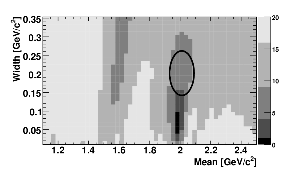
After adding the to the nominal model we repeat the same procedure for an additional tensor particle. We find that the has a significant contribution. The results of the likelihood scans are shown in Fig. 2 in terms of , where corresponds to the minimal value obtained in the particular scan. To conclude the search for possible resonant contributions we add all well established resonances [16] and check if the likelihood increases. We do not find any other significant resonant contribution but as we cannot exclude small contributions from the , , , , and resonances, we assign model uncertainties (see Sec. III.6) due to not taking these resonances into account.
Figure 2:
Two-dimensional scans of
(gray scale)
as a function of the mass and the width of an additional resonance. These scans were performed to look for an additional scalar resonance (left) and an additional tensor resonance (right). The baseline model of the scans for additional scalar resonances contains , , and NR intermediate states. The baseline model of the scans for additional tensor resonances contains , , NR, and intermediate states. The
ellipses indicate the world average parameters [16] for the and resonances that are added to the model.
III.5 Results
The maximum-likelihood fit of candidates results in a event yield of and a continuum yield of , where the uncertainties are statistical only.
The symmetrized and square Dalitz plots of a signal DP-model MC sample generated with the result of the fit to data are shown in Fig. 3.
Figure 4 shows plots of , , and the NN for isolated signal and continuum background events obtained by the [21] technique.
Figure 5 shows projections of the data onto the invariant masses and .
Figure 3:
Symmetrized (left) and square (right) DP for MC simulated signal events using the amplitudes obtained from the fit to data. The low population in bins along the edge of the symmetrized DP is due to the fact that the phase space boundaries do not coincide with the histogram bin boundaries.
Figure 4: (color online). (points with error bars) and PDFs (histograms) of the discriminating variables: (top), (middle), and NN (bottom), for signal events (left) and continuum events (right).
Below each bin are shown the residuals, normalized in error units. The horizontal dotted and full lines mark the one- and two-standard deviation levels, respectively.
Figure 5: (color online). Projections onto (left) and (right). On-resonance data are shown as points with error bars while the dashed (dotted) histogram represents the signal (continuum) component. The solid-line histogram is the total PDF. Below each bin are shown the residuals, normalized in error units. The horizontal dotted and full lines mark the one- and two-standard deviation levels, respectively.
When the fit is repeated with initial parameter values randomly chosen within wide ranges above and below the nominal values for the magnitudes and within the interval for the phases, we observe convergence towards two solutions with minimum values of the negative log likelihood function separated by units. In the following, we refer to them as
Solution 1 (the global minimum) and Solution 2 (a local minimum). No other local minima were found.
In the fit, we measure directly the relative magnitudes and phases of the different components of the signal model. The magnitude and phase of the NR amplitude are fixed to and , respectively, as a reference.
In Fig. 6 we show likelihood scans of the isobar magnitudes and phases of all the resonances, where both solutions can be noticed. Each of these scans is obtained by fixing the corresponding isobar parameter at several consecutive values, for each of which
the fit to the data is repeated.
The measured relative amplitudes
are used to extract the fit fraction defined as
(31)
where , which varies from 1 to 5, represents an intermediate state.
Each fit fraction is a sum of three identical contributions, one for each pair of . The indices and run from 1 to 15, as each of the five resonances contributes to three pairs of , which correspond to the three terms (, , and ) in each sum in the numerator of Eq. (31).
The dynamical amplitudes are defined in Sec. III.1 and the terms
(32)
are obtained by integration over the DP.
The total fit fraction is defined as the algebraic sum of all fit fractions. This quantity is not
necessarily unity due to the potential presence of net constructive or destructive interference.
In order to estimate the statistical significance of each resonance, we
evaluate the difference between the log-likelihood of the nominal fit and that of a fit where the magnitude of the amplitude of the resonance is set to (this difference can be directly read from the likelihood scans as a function of magnitudes in Fig. 6). In this case the phase of the resonance becomes meaningless, and we therefore account for two degrees of freedom removed from the fit.
The value is used to evaluate the -value for degrees of freedom;
we determine the equivalent one-dimensional significance from this -value.
The results for the phase and the fit fraction are given in Table 2 for the
two solutions; the change in likelihood when the amplitude of the resonance is set to and the resulting statistical significance of each resonance is given for Solution 1.
As the fit fractions are not parameters of the PDF itself, their statistical errors are obtained from the coverage intervals of the fit-fraction distributions obtained from a large number of pseudoexperiments generated with the corresponding solution (1 or 2). As observed in other three-kaon modes [6, 9, 7, 8, 10], the total FF significantly exceeds unity.
Table 2:
Summary of measurements of the quasi-two-body parameters. The quoted uncertainties are statistical only.
The change in the log-likelihood () corresponds to the case where the magnitude of the amplitude of the resonance is set to 0. This number is used for the estimation of the statistical significance of each resonance.
Mode
Parameter
Solution 1
Solution 2
FF
Phase [rad]
-
Significance []
-
FF
Phase [rad]
-
Significance []
-
FF
Phase [rad]
-
Significance []
-
NR
FF
Phase [rad]
-
Significance []
-
FF
Phase [rad]
-
Significance []
-
Total FF
In Table 2 it can be seen that the two solutions differ mostly in the fraction assigned to the NR and the components.
Solution 1 corresponds to a small FF of the and a large value for the NR, and Solution 2 has a large fraction and a smaller NR fraction. Other three-kaon modes [6, 9, 7, 8, 10] favor the behavior of Solution 1.
Figure 6:
(color online). One-dimensional scans of as a function of magnitudes (left) and phases (right) of the resonances , , , and (top to bottom). The horizontal dashed lines mark the one- and two-standard deviation levels.
Generalizing Eq. (31), we obtain the interference fractions among the intermediate decay modes and
(33)
which are given in Table 3 for Solution 1. Unlike the total FF defined above, the elements of this matrix sum to unity. The large destructive interference between the and the NR components appears clearly in the table.
This is possible due to the large overlap in phase space between the exponential NR term and the broad tail of the resonance above the threshold.
Table 3: The interference fractions among the intermediate decay amplitudes for Solution 1. Note that the diagonal elements are those defined in Eq. (31) and detailed in Table 2. The lower diagonal elements are omitted since the matrix is symmetric.
NR
NR
Using the relative fit fractions, we calculate the branching fraction for the intermediate mode as
(34)
where is the total inclusive branching fraction:
(35)
We estimate the average efficiency using a fully reconstructed DP-model MC sample generated with the parameters found in data.
The results of the branching fraction measurements are shown in Table 4. As a cross check we attempt to compare our measured branching fractions to results from other measurements; however, many of the branching fractions for the decay into kaons of the resonances included in our model are not (or are only poorly) measured (marked as “seen” in Ref. [16]). An exception is the charmonium state , for which the measured value is [16]. We can then use the BABAR measurement of [22] to calculate , which is consistent with our measured branching fraction, given in Table 4.
An interesting conclusion from this first amplitude analysis of the decay mode is that we do not need to include a broad scalar resonance, as has been done in other measurements [6, 9, 7, 8, 10], to describe the data. The peak in the invariant mass between and can be described by the interference between the resonance and the nonresonant component. However minor contributions from the and resonances to this structure cannot be excluded.
Table 4: Summary of measurements of branching fractions (). The quoted numbers are obtained by multiplying the corresponding fit fraction from Solution 1 by the measured inclusive branching fraction. The first uncertainty is statistical, the second is systematic, and the third represents the signal DP-model dependence.
Mode
[]
Inclusive
,
,
,
,
,
III.6 Systematic uncertainties
Systematic effects are divided into model and experimental uncertainties. Details on how they have been estimated are given below and the associated numerical values are summarized in Table 5.
III.6.1 Model uncertainties
We vary the mass, width, and any other parameter of all isobar fit components within their errors, as quoted in Table 1, and assign the observed differences in our observables as the first part of the model uncertainty (“Model” in Table 5).
To estimate the contribution to from resonances that are not included in our signal model but cannot be excluded statistically, namely the , , , , and resonances, we perform fits to pseudoexperiments that include these resonances. The masses and the widths are taken from [16], except for the for which we take the values from [23]. We generate pseudoexperiments with the additional resonances, where the isobar magnitudes and phases have been determined in fits to data, and fit these datasets with the nominal model. We assign the induced shift in the observables as a second part of the model uncertainty.
III.6.2 Experimental systematic uncertainties
To validate the analysis procedure, we perform fits on a large number of pseudoexperiments generated with the measured yields of signal events and continuum background. The signal events are taken from fully reconstructed MC that has been generated with the fit result to data. We observe small biases in the isobar magnitudes and phases. We correct for these biases by shifting the values of the parameters and assign to this procedure a systematic uncertainty, which corresponds to half the correction combined in quadrature with its error. This uncertainty accounts also for correlations between the signal variables, wrongly reconstructed events, and effects due to the limited sample size (“Fit Bias” in Table 5).
From MC we estimate that there are six background events in our data sample. To determine the bias introduced by these events, we add background events from MC to our data sample, and fit it with the nominal model. We then assign the observed differences in the observables as a systematic uncertainty (“-bkg” in Table 5).
We assign a systematic uncertainty for all fixed PDF parameters by varying them within their uncertainties according to the covariance matrix.
We vary the histogram PDFs, i.e., the SDP PDF for continuum and the NN PDF for signal (“Discr. Vars” in Table 5).
The dependence of the SDP PDF for continuum was found to be negligible.
We account for differences between simulation and data observed in the control sample (“MC-Data” in Table 5).
These differences were estimated by propagating the differences, in the control sample, between background-subtracted data and signal MC, into the fit PDFs.
For the branching fraction measurement, we assign a systematic uncertainty due to the error on the calculation of (“” in Table 5) and to the reconstruction efficiency. We correct the reconstruction efficiency by the difference between the efficiency found in a dedicated data sample and that found in simulation.
We assign the uncertainty on the correction as a systematic error (“ reco” in Table 5).
Table 5: Summary of systematic uncertainties. The model uncertainty is dominated by the variation of the line shapes due to the contribution of the poorly measured .
Parameter
Fit bias
-bkg
Discr. Vars
MC-Data
reco
Sum
Model
FF
-
-
FF
-
-
FF
-
-
FF NR
-
-
FF
-
-
Ph [rad]
-
-
Ph [rad]
-
-
Ph [rad]
-
-
Ph [rad]
-
-
IV Time-dependent analysis
In Sec. IV.1 we describe the proper-time distribution used to extract the time-dependent asymmetries.
In Sec. IV.2 we explain the selection
requirements used to obtain the signal candidates and
suppress backgrounds. In Sec. IV.3 we describe the fit method
and the approach used to account for experimental effects.
In Sec. IV.4 we present the results of the fit and finally, in Sec. IV.5 we discuss systematic uncertainties in the results.
IV.1 Proper-time distribution
The time-dependent asymmetries are functions of the proper-time difference between a fully reconstructed decay () and the other meson decay in the event (), which is partially reconstructed. The observed decay rate is the physical decay rate modified to include tagging imperfections, namely and ; the former
is the rate of correctly assigning the flavor of the meson, averaged over and ,
and the latter is the difference between for and .
The index denotes different quality categories of the tag-flavor assignment.
Furthermore the decay rate is convolved with the per-event resolution , which is described by the sum of three Gaussians and depends on and its error .
For an event with tag flavor , one has
(36)
where is defined to be () for (), is the mean lifetime, and is the mixing frequency [16]. The widths of the and the are assumed to be the same.
IV.2 Event selection and backgrounds
We reconstruct candidates either from three candidates, or from two and one , where the candidates are formed from pairs of photons. The vertex fit requirements are the same as in the amplitude analysis, and also the requirement that the charged pions of at least one of the have hits in the two inner layers of the vertex tracker.
The candidates in the submode must have mass within of the nominal mass [16] and decay length with respect to the vertex between and .
In addition, combinatorial background is suppressed in both submodes by imposing that the angle between
the momentum vector of each candidate
and the vector connecting the beamspot and the vertex is smaller than 0.2 radians.
Each decaying to charged pions in the submode
is required to have decay length between and cm and invariant mass less than from the world average mass [16]. The decaying to neutral pions in the submode must have invariant mass between and . Additionally, the neutral pions are selected if they have invariant mass between and and if the photons have energies greater than in the laboratory frame and a lateral energy deposition profile in the electromagnetic calorimeter consistent with that expected for an electromagnetic shower (lateral moment [24] less than ).
The fact that we do not model any PDF using sideband data allows a loose requirement on and in the time-dependent analysis, namely, and .
In case of multiple candidates passing the selection, we proceed in the same way as in the amplitude analysis.
We use the same NN as in the amplitude analysis to suppress continuum background.
With the above selection criteria, we obtain signal reconstruction efficiencies of and for the and submodes, respectively. These efficiencies are determined from a DP-model MC sample generated using the results of the amplitude analysis.
We estimate from MC that of the selected signal events are misreconstructed for , while the figure is in ,
and we do not treat these events differently from correctly reconstructed events.
Because of the looser requirements, there are more background events from decays than in the amplitude analysis, in particular in the submode. These backgrounds are included in the fit model and are summarized in Table 6.
As the analysis is phase-space integrated, we cannot model the resonance separately, and its contribution to the asymmetries could cloud deviations in the charmless contributions.
We therefore apply a veto around the invariant mass of this charmonium state.
Table 6: Summary of background modes included in the fit model of the time-dependent analysis. The expected number of events takes into account the branching fractions () and efficiencies. In case there is no measurement, the branching fraction of an isospin-related channel is used. All the fixed yields are varied by for systematic uncertainties.
Submode
Background mode
Varied
[]
Number of events
no
no
no
yes
not applicable
yes
not applicable
no
no
no
no
no
yes
not applicable
yes
not applicable
IV.3 The maximum-likelihood fit
We perform an unbinned extended maximum-likelihood fit to extract the event yields along with
the and parameters of the time-dependent analysis.
The fit uses as variables , , the NN output, , and . The selected on-resonance data sample is assumed to consist of signal, continuum background, and backgrounds from decays. Wrongly reconstructed signal events are not considered separately. The likelihood function for event is the sum
(37)
where stands for the species (signal, continuum background, one for each background category) and is the corresponding yield; , , and are the tag flavor, the tagging category, and the physics category, respectively.
To determine and we use the flavor-tagging
algorithm of Ref. [25]. This algorithm combines several
different signatures, such as charges, momenta, and decay
angles of charged particles in the event to achieve optimal
separation between the two flavors. This produces six
mutually exclusive tagging categories.
We also retain untagged events in a seventh category;
although these events do not contribute to the measurement
of the time-dependent CP asymmetry they do provide
additional sensitivity for the measurement of direct violation [26].
The two physics categories correspond to and decays.
The PDF for species evaluated for event is given by the product of individual PDFs:
(38)
To take into account the different reconstruction of the two submodes,
we use separate PDFs for the two physics categories. Separate NN and
PDFs are included for each tagging category within each physics
category. The separate PDFs for the two physics categories allow
us to fit the
and parameters either separately for the two submodes, or together.
The total likelihood is given by
(39)
IV.3.1 PDFs
The signal PDF for is given in Eq. (36).
Parameters that depend solely on the tag side of the events (namely, and ) are taken from the analysis of decays [27]. On the other hand, parameters that depend on the signal-side reconstruction, due to the absence of direct tracks from the decay, cannot be taken from modes that include such direct tracks. This is the case for the parameters that describe the resolution function, which are found in a fit to simulated events. A systematic uncertainty for data-MC differences is assigned using the control sample , as explained in Sec. IV.5.
For continuum events we use a zero-lifetime component. This parametrization is convolved with the
same resolution function as for signal, with different parameters that are varied in the fit to data.
The parameters of this PDF are not separated in the tagging categories.
The small contribution from events is well described by the tails of the resolution function.
For background events we use the signal PDF, with resolution parameters
from the BABAR analysis [27].
The parameters and are set to zero and varied
to assign a systematic uncertainty.
IV.3.2 Description of the other variables
The and distributions of signal events are parametrized by an asymmetric Gaussian with power-law tails, as given in Eq. (24), and, for , a small additional component, parameterized by an ARGUS shape function [20], to correctly describe misreconstructed events. The means in these two PDFs for events are allowed to vary in the fit to data, and the other parameters are taken from MC simulation.
For the NN distributions of signal we use histogram PDFs taken from MC simulation for each physics and tagging category.
The , , and NN PDFs for continuum events are parametrized by an ARGUS shape function, a straight line and the sum of power functions from Eq. (28), respectively. All continuum parameters, except for
and
of the NN PDF, are allowed to vary in the fit. All the fixed parameters are varied, within the uncertainties found in a fit to sideband data, to estimate systematic errors.
All the background PDFs are described by fixed histograms taken from MC simulation.
IV.4 Results
The maximum-likelihood fit of candidates in the submode and candidates in the submode results in the event yields detailed in Table 7.
Table 7: Event yields for the different event species, resulting from the maximum-likelihood fit for the time-dependent analysis. “ () bkg” represents background from charged (neutral) decays. Quoted uncertainties are statistical only.
Species
Signal
Continuum
bkg
bkg
The fit result for the time-dependent -violation parameters and is
where the uncertainties are statistical only. The correlation between and is .
We use the fit result to create of the signal distributions of , the time-dependent asymmetry, and the discriminating variables. Figure 7 shows the for the combined fit result and for the individual submodes.
Figure 8 shows the signal distributions and Fig. 9 the continuum background distributions of the discriminating variables.
The distributions shown in these three figures illustrate the good agreement between the data and the fit model.
We scan the statistical-only likelihood of the parameter for both submodes and for the combined fit. The result, on the left-hand side of Fig. 10, shows a sizable difference between the values for the two submodes;
the level of consistency, conservatively estimated from the sum of the two individual likelihood scans, is approximately (a -value of with degrees of freedom).
This value is obtained including only the dominant statistical uncertainty and neglecting the small correlation between the -violation parameters.
The results obtained when and are allowed to vary individually for each of the submodes are , for and , for . In both cases the quoted uncertainties are statistical only.
As there is some correlation between the and parameters, we perform a two-dimensional statistical likelihood scan of the combined likelihood, which is then convolved by the systematic uncertainties on and (systematic uncertainties are discussed in Sec. IV.5.)
The result is shown on the right-hand side of Fig. 10.
We find that conservation is excluded at standard deviations, and thus, for the first time, we measure an evidence of violation in decays.
The difference between our result and that from is less than standard deviations.
The scan also shows that the result is close to the physical boundary, given by the constraint .
Figure 7: (color online). Signal (points with error bars) and PDFs (histograms) of (left) and the derived asymmetry (right) for the submode (top), the submode (middle), and the combined fit (bottom). In the distributions on the left-hand side, points marked with and solid lines correspond to decays where is a meson; points marked with and dashed lines correspond to decays where is a meson.
Points of the asymmetry that are outside the range of a figure are marked by arrows.
Figure 8:
(color online). Signal (points with error bars) and PDFs (histograms) of the discriminating variables: (top), (middle), and the NN output (bottom) for the submode (left) and for the submode (right). Below each bin are shown the residuals, normalized in error units. The horizontal dotted and full lines mark the one- and two-standard deviation levels, respectively.
Figure 9: (color online). Continuum (points with error bars) and PDFs (histograms) of , , the NN output, and (top to bottom). Plots on the left-hand side correspond to the submode, and on the right-hand side to the submode. In the distributions, points marked with and solid lines correspond to decays where is a meson; points marked with and dashed lines correspond to decays where is a meson. Below each bin are shown the residuals, normalized in error units. The horizontal dotted and full lines mark the one- and two-standard deviation levels, respectively.
Figure 10: (color online). One-dimensional statistical scan of as a function of (left) and the two-dimensional scan, including systematic uncertainty, as a function of and (right). In the left-hand plot, red points marked with correspond to the submode, blue points marked with to the submode, and black points marked with to the combined fit. In the right-hand plot,
the gray scale is given in units of .
The result of the BABAR analyses of decays [27] is indicated as a white ellipse and the physical boundary () is marked as a gray line. The scan appears to be trimmed on the lower left since the PDF becomes negative outside the physical region (i.e., the white region does not indicate that the scan flattens out at 5).
IV.5 Systematic uncertainties
The systematic uncertainties are summarized in Table 8. The “” uncertainty accounts for the limited size of the simulated data samples used to create the PDFs. The “” uncertainty propagates the experimental uncertainty in the measurement of tag-side-related quantities taken from [27] to our measurement. The “-bkg” contribution results from the uncertainty in the content and the branching fractions of fixed yields in the model of background from decays. The dominant “MC-Data: ” systematic uncertainty is due to possible differences between data and simulation
concerning the procedure used to obtain the signal decay vertex from tracks originating from decays.
We quantify this uncertainty using the control sample by comparing the difference between values obtained with and without the in data and simulation. We then propagate the observed differences and their uncertainties to the resolution function. We use this new resolution function to refit the data and obtain an estimate of the effect on and . We also use the samples and to estimate simulation-data differences for the other variables in the submodes and , respectively. This contribution is referred to as “MC-Data: Discr. Vars” in Table 8. The “Fit Bias” uncertainty is evaluated using fits to fully reconstructed MC samples. It accounts for effects from wrongly reconstructed events and correlations between fit variables. The “Vetoes” uncertainty is related to the veto on the invariant mass. It is evaluated using events that pass the veto in pseudo-experiments studies. Finally, the “Misc” uncertainty includes contributions from doubly-Cabibbo-suppressed decays, silicon vertex tracker alignment, and the uncertainties in the boost of the . These contributions are taken from the BABAR analysis [27].
Table 8: Summary of systematic uncertainties on the and parameters.
Source
-bkg
MC-Data:
MC-Data: Discr. Vars
Fit Bias
Vetoes
Misc
Sum
V SUMMARY
We have performed the first amplitude analysis of events and measured the total inclusive branching fraction to be , where the first uncertainty is statistical, the second is systematic, and the third represents the signal DP-model dependence. We have identified the dominant contributions to the DP to be from , , , and a nonresonant component, and measured the individual fit fractions and phases of each component. We do not observe any significant contribution from the so-called resonance seen in, for example, [6]. The peak in the invariant mass between and can be described by the interference between the resonance and the nonresonant component. We see some hints from the and resonances that could also contribute to this structure, but due to limited sample size we cannot make a significant statement. Future investigations of the system could shed more light on the situation.
Furthermore we have performed an update of the phase-space-integrated time-dependent analysis of the same decay mode, using and decays, with the final BABAR dataset. We measure the -violation parameters to be and , where the first quoted uncertainty is statistical and the second is systematic.
These measured values are consistent with and supersede those reported in Ref. [3]. They are compatible within two standard deviations with those measured in tree-dominated modes such as , as expected in the SM. For the first time, we report evidence of violation in decays; conservation is excluded at standard deviations including systematic uncertainties.
ACKNOWLEDGMENTS
We are grateful for the
extraordinary contributions of our PEP-II colleagues in
achieving the excellent luminosity and machine conditions
that have made this work possible.
The success of this project also relies critically on the
expertise and dedication of the computing organizations that
support BABAR.
The collaborating institutions wish to thank
SLAC for its support and the kind hospitality extended to them.
This work is supported by the
US Department of Energy
and National Science Foundation, the
Natural Sciences and Engineering Research Council (Canada),
the Commissariat à l’Energie Atomique and
Institut National de Physique Nucléaire et de Physique des Particules
(France), the
Bundesministerium für Bildung und Forschung and
Deutsche Forschungsgemeinschaft
(Germany), the
Istituto Nazionale di Fisica Nucleare (Italy),
the Foundation for Fundamental Research on Matter (The Netherlands),
the Research Council of Norway, the
Ministry of Education and Science of the Russian Federation,
Ministerio de Ciencia e Innovación (Spain), and the
Science and Technology Facilities Council (United Kingdom).
Individuals have received support from
the Marie-Curie IEF program (European Union), the A. P. Sloan Foundation (USA)
and the Binational Science Foundation (USA-Israel).
References
[1]
Y. Grossman and
M. P. Worah,
Phys. Lett. B 395,
241 (1997).
[2]
H.-Y. Cheng,
C.-K. Chua, and
A. Soni,
Phys. Rev. D 72,
094003 (2005).
[3]
B. Aubert et al.
(BABAR), Phys. Rev.
D 76, 091101
(2007a).
[4]
K.-F. Chen et al.
(Belle), Phys. Rev. Lett.
98, 031802
(2007).
[5]
T. Gershon and
M. Hazumi,
Phys. Lett. B 596,
163 (2004).
[6]
B. Aubert et al.
(BABAR), Phys. Rev.
D 74, 032003
(2006).
[7]
B. Aubert et al.
(BABAR), Phys. Rev. Lett.
99, 161802
(2007b).
[8]
B. Aubert et al.
(BABAR) (2008),
presented at ICHEP 2008, eprint arXiv:0808.0700.
[9]
A. Garmash et al.
(Belle), Phys. Rev.
D 71, 092003
(2005).
[10]
Y. Nakahama et al.
(Belle), Phys. Rev.
D 82, 073011
(2010).
[11]
B. Aubert et al.
(BABAR), Phys. Rev. Lett.
99, 221801
(2007c).
[12]
B. Aubert et al.
(BABAR), Phys. Rev. D. RC
79, 051101
(2009a).
[13]
N. Rey-Le Lorier
and D. London,
Phys.Rev. D 85,
016010 (2012).
[14]
B. Aubert et al.
(BABAR), Nucl. Instrum. Methods
Phys. Res. A 479, 1
(2002).
[15]
J. Blatt and
V. E. Weisskopf,
Theoretical Nuclear Physics (J.
Wiley, New York, 1952).
[16]
C. Amsler et al.
(Particle Data Group), Phys.
Lett. B 667, 1
(2008).
[17]
S. M. Flatte,
Phys. Lett. B 63,
224 (1976).
[18]
M. Ablikim et al.
(BES), Phys. Lett.
B 607, 243
(2005).
[19]
P. Gay,
B. Michel,
J. Proriol, and
O. Deschamps
(1995), prepared for 4th International
Workshop on Software Engineering and Artificial Intelligence for High-energy
and Nuclear Physics (AIHENP 95), Pisa, Italy, 1995.
[20]
H. Albrecht et al.
(ARGUS), Z. Phys.
C 48, 543 (1990).
[21]
M. Pivk and
F. R. Le Diberder,
Nucl. Instrum. Methods Phys. Res.
A 555, 356
(2005).
[22]
B. Aubert et al.
(BABAR), Phys. Rev.
D 80, 112001
(2009b).
[23]
P. del Amo Sanchez
et al. (BABAR),
Phys. Rev. D 83,
052001 (2011).
[24]
A. Drescher
et al., Nucl. Instrum. Methods Phys. Res.
A 237, 464
(1985).
[25]
B. Aubert et al.
(BABAR), Phys. Rev. Lett.
94, 161803
(2005).
[26]
S. Gardner and
J. Tandean,
Phys. Rev. D69,
034011 (2004).
[27]
B. Aubert et al.
(BABAR), Phys. Rev.
D 79, 072009
(2009c).