Theory of the Casimir effect for graphene at finite temperature

The quasiparticles in graphene[1] obey a linear dispersion law $\omega=v_{F}k$ ($v_{F}\approx c/300$ is a Fermi velocity, $c$ is a speed of light) at energies less than $2$ eV. Graphene’s $2+1$ - dimensionality and quasi-relativistic Dirac model for its quasiparticles make it possible to derive the Casimir effect properties of graphene systems from general constraints and principles of quantum field theory.

Casimir effect in graphene systems was studied in different papers [2]-[8]. Finite-temperature results were obtained in Refs. [4] and [5]. In the current paper we follow the formalism developed in Ref.[5], an alternative derivation of the reflection coefficients is presented, the relation to Feynman diagrams is discussed. First we derive the expressions for the components of the polarization operator of quasiparticles in a graphene layer at finite temperature and derive the reflection coefficients of a flat graphene layer from the solutions of the boundary problems for vector potentials. The free energy is given then in two equivalent forms: in terms of reflection coefficients and closed Feynman diagrams. Finally we study the exceptional properties of the free energy of a flat graphene layer – parallel flat metal system at finite temperatures.

We use the coordinates $x^{3}$ and $z$ interchangeably throughout the paper. When needed we select the coordinate $y$ along a direction of the wavevector ${\mathbf{q}}=(q^{1},q^{2})$ (longitudinal direction) and the coordinate $x$ along a transverse direction. We use $\hbar=c=k_{B}=1$.

The model is described by the following classical action (assuming graphene plane lying at $x^{3}=0$)

with

Here $\mu$ is a chemical potential, $m$ is a mass gap of quasiparticle excitations, $v_{F}\approx 1/300$ is a Fermi velocity. Since there are $N=4$ species of fermions in graphene, the gamma matrices are in fact $8\times 8$, being a direct sum of four $2\times 2$ representations (with two copies of each of the two inequivalent ones), $\gamma_{0}^{2}=-(\gamma^{1,2})^{2}=1$. The Maxwell action is normalized in such a way that

In Minkowski space the one-loop polarization operator can be expressed in momentum space as

where the propagator of the quasiparticles in graphene reads

Note that for $\mu=m=0$ the pole of the propagator yields the linear dispersion law for quasiparticles in graphene: $q_{0}=v_{F}|{\bf q}|$. Here ${\mathbf{q}}=(q^{1},q^{2})$, $\not{q}=\gamma^{1}q_{1}+\gamma^{2}q_{2}$. Vectors with tilde are rescaled by multiplying the spatial components with $v_{F}$, i.e., $\tilde{p}^{j}\equiv\eta^{j}_{i}p^{i}=(p_{0},v_{F}{\mathbf{p}})$, $\eta=\textrm{diag}(1,v_{F},v_{F})$.

To introduce the temperature in (3) we perform the rotation to the Matsubara frequencies

use the Feynman parametrization

and subsequently change the variables in (3) in the spatial part of the loop–integration: ${\bf q}\to{\bf q}+x{\bf p}$. Then we come to

where $M_{0}^{2}=m^{2}+v_{F}^{2}{\mathbf{q}}^{2}-x(1-x)v_{F}^{2}{\mathbf{p}}^{2}$, and

In equation (6) we introduced the integration variable $\Theta$.

In analogy we get

Summation over the fermion Matsubara frequencies can be made explicitly by making use of the identities

where in (11) we substituted $b=p_{0}x-\mu$.

To perform the integration over $\Theta$ it is convenient to use the identity $\partial_{s}\tanh s={\rm sech}^{2}s$. Finally we arrive at the following representation for $\Pi_{00}$ and $\Pi_{{\rm tr}}\equiv\Pi_{m}^{m}$:

where $\Theta_{0}\equiv\sqrt{m^{2}-x(1-x)(p_{0}^{2}-v_{F}^{2}{\bf p}^{2})}$, $b=p_{0}x-\mu$, and

Here $p_{3}^{2}\equiv p_{0}^{2}-{\mathbf{p}}^{2}$. We remind that $N$ is the number of fermion species, $N=4$ for graphene. Parity-odd contributions to the polarization tensor cancel out between different species, while the parity-even contributions add up.

In this section we find reflection coefficients for transverse electric (TE) and transverse magnetic (TM) modes. The equations

lead to the conditions

where [9]

$u^{j}=\delta^{j0}$ and $i,j=0,1,2$. Here $A$, $B$ are scalar functions.

Let’s consider the condition

In fact, the condition (19) is quite convenient for a description of transverse electric and transverse magnetic modes of the propagating electromagnetic wave.

A nonzero $A_{x}$, the condition $\partial_{x}A_{x}=0$ and the conditions $A_{y}=A_{z}=A_{0}=0$ describe the propagation of a TE electromagnetic wave (the electric field is parallel to the surface $z=0$) since $E_{x}\sim A_{x}$. Here the direction perpendicular to the wave vector of the electromagnetic wave under consideration $(0,p_{y},p_{z})$ is denoted by $x$.

For the TE wave we have:

and

Here $p_{z}^{2}=p_{0}^{2}-p_{y}^{2}$. From the continuity of potentials at $z=0$ we obtain $1+r_{TE}=t_{TE}$. Now one substitutes (20) and (21) into (16) and uses (22) to obtain:

The conditions $A_{x}=A_{z}=0$, $p_{0}A_{0}=p_{y}A_{y}$ describe the transverse magnetic (TM) wave. This choice of vector potentials describes TM wave since $E_{z}\sim\partial_{z}A_{0}$ or $B_{x}\sim\partial_{z}A_{y}$. For $A_{0}$ we have:

and

where $\tilde{p}_{z}^{2}=p_{0}^{2}-v_{F}^{2}p_{y}^{2}$. One substitutes (24) and (25) into (16) and uses (26) to obtain:

Since $E_{z}\sim\partial_{z}A_{0}$ the reflection coefficient for the TM mode is equal

The reflection coefficients (23) and (28) are reflection coefficients of transverse electric and transverse magnetic modes respectively.

One can also rewrite the reflection coefficients in terms of the polarization tensor components

The two conditions follow from gauge invariance:

which yield after Wick rotation

and the property

The reflection coefficients can be rewritten in the form:

In the gauge $A_{0}=0$ the longitudinal part of the free photon propagator $D^{L}$ has the form

the transverse part of the free photon propagator $D^{T}$ has the form:

Let’s choose coordinate axes in the plane of a graphene sheet so that $p_{y}={|\bf p|}$. Lifshitz free energy [11] has the form:

where $\omega_{n}=2\pi nT$ are Matsubara frequencies, the respective transverse magnetic and transverse electric reflection coefficients from two parallel flat surfaces separated by a vacuum slit $a$ are denoted by $r_{TM}$ and $r_{TE}$. For the ideal metal $r_{TM}=1$, $r_{TE}=-1$. Note, however, that some exact results in complicated geometries[12]-[13] can be essentially different from the approximations based on Lifshitz formula for two parallel plates (see also Ref.[14] which considers sphere-plane system).

From the comparison of the formula (36) and expressions (32) – (35) it follows that for graphene – ideal metal, graphene – graphene the Lifshitz theory takes into account the set of closed Feynman one loop diagrams responsible for interaction between the two materials separated by a vacuum slit. The longitudinal and the transverse parts of the photon propagator enter two different sets of closed one loop diagrams for the free energy and multiplied in these Feynman diagrams by the longitudinal and the transverse components of the polarization operator $\Pi_{yy}$ and $\Pi_{xx}$ respectively. Lifshitz type formulas result from the sum over closed Feynman one loop diagrams with $z=a$ or $z=2a$ in photon propagators connecting the two sheets of graphene or a graphene sheet interacting with an ideal metal respectively. Inside each graphene layer the sum of RPA diagrams is taken into account by factors in round parentheses in (32), (33). The division of the free energy into longitudinal and transverse parts in terms of respective parts of photon Green’s functions and polarization operator is equivalent to a division into TM and TE parts described by the reflection coefficients $r_{\rm TM}$ and $r_{\rm TE}$ in the Lifshitz approach.

Let’s assume $m=0$, $\mu=0$ [10]. For $|{\bf p}|\to 0$ one gets:

and reflection coefficients have the form:

Zero Matsubara TM and TE terms yield the following high-temperature behavior of the free energy (36) in graphene – ideal metal system:

Here

is the high-temperature asymptotics of the metal – metal system with a Drude model of the permittivity used [15]-[25], which is equal to one half of the high-temperature asymptotics in the metal – metal system with the ideal boundary conditions or the plasma model of the permittivity used [26] (see Ref.[27] for a review). The zero frequency TE Matsubara term is suppressed by a factor $\alpha Nv_{F}^{2}$ and additional power of $1/(Ta)$.

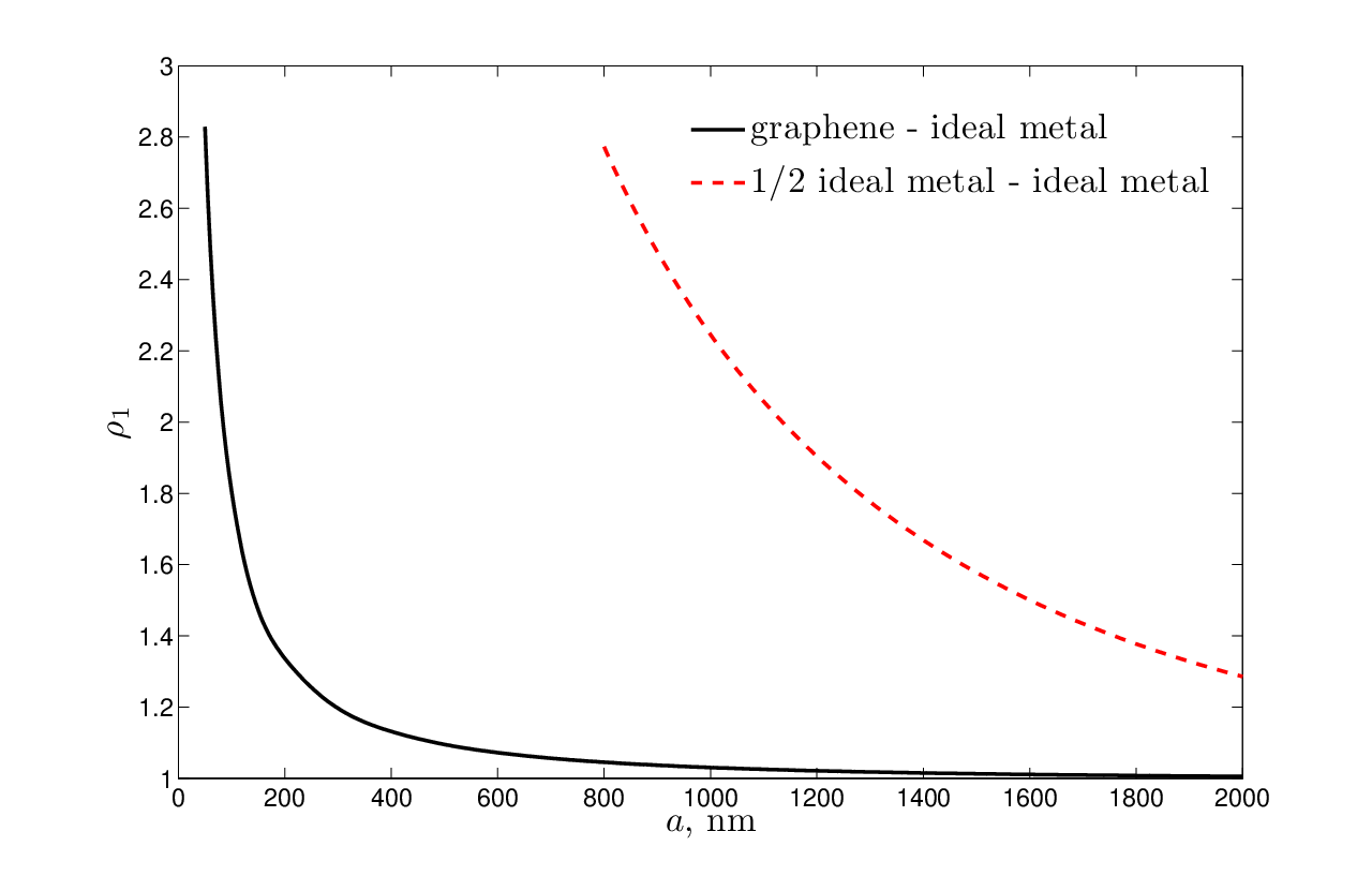
The typical region of validity of the high-temperature asymptotics for the metal–metal system is $4\pi Ta\gg 1$. However, due to a suppression of nonzero Matsubara terms by the coupling constant $\alpha$ the free energy in a graphene – metal system approaches the high-temperature asymptotics $-T\zeta(3)/(16\pi a^{2})$ much quicker and at shorter separations than in the metal – metal case (see next section).

Note that in the graphene – ideal metal system the high-temperature asymptotics is derived from the first principles of quantum field theory.

It is often desirable to have an accurate analytical approximation of the exact result at different separations. We present such an expression for the sum of nonzero Matsubara terms in this section.

To obtain an appropriate analytical expression we first note that at separations $H\gg v_{F}$ one can put $v_{F}=0$ in any nonzero Matsubara term. It is possible due to the exponential factor in the Lifshitz formula which effectively restrains the integration over impulse to $a|{\bf p}|\lesssim 1$. In this case contribution of the type of $v_{F}^{2}(a|{\bf p}|)^{2}$ can be neglected compared to $(ap_{0})^{2}=(2\pi naT)^{2}$ due to the smallness of the parameter $v_{F}$.

In the finite temperature sum of nonzero Matsubara terms in the Lifshitz formula one can use the reflection coefficients taken at zero temperature. The corrections due to finite temperature are suppressed for nonzero Matsubara terms, so we neglect them in the leading approximation.

Under two mentioned above approximations and the condition $m=\mu=0$ the reflection coefficients of a single graphene layer at zero temperature have the form:

Due to smallness of the reflection coefficients (both being of the order of $\alpha$) we can take just the first term in the expansion of the logarithm in the Lifshitz formula. Note, however, that expansion of the TM reflection coefficient in $\alpha$ is not legitimate, as will become evident below (see (46)).

The sum of nonzero Matsubara terms in (36) in this approximation in the TM case with $r^{(1)}_{\rm TM}=r_{\rm TM}^{T=0}$ (40) and $r^{(2)}_{\rm TM}=1$ equals to

here $s_{1}=\sqrt{\omega_{n}^{2}+|{\bf p}|^{2}}$ and $g\equiv 32Ta/(\alpha N)$, $E_{1}$ stands for the standard exponential integral function. It is convenient to reexpress the result (42) in an integral form. For this purpose one has to differentiate (42) over $H$, assuming $H$ as an independent parameter for the moment, calculate the sum over $n$ and then integrate back over $H$ (the integration constant is fixed as zero at $H\to\infty$). Thus one obtains

The TE part of the nonzero Matsubara terms of the Lifshitz formula with the coefficients $r^{(1)}_{TE}=r_{TE}^{T=0}$ from (41) and $r^{(2)}_{TE}=-1$ gives the following contribution in the leading order in $\alpha$

Thus, the complete result for the sum of nonzero Matsubara TM and TE terms in the approximation described above is given by (43) and (44):

Consequently, the leading $v_{F}=0$ contribution to the free energy is the sum $-T\zeta(3)/(16\pi a^{2})$ + $\Delta\mathcal{F}$. It can be used for the comparison of the theory and experiment with $1\%$ accuracy for all separations at $T=300$K.

From (43) and (44) one gets the energy at $T=0$ in the limit $v_{F}\to 0$:

where the non analyticity in $\alpha$ comes from the TM mode.

Fig.1 clearly demonstrates that the free energy of a graphene – metal system approaches the high-temperature asymptotics $-T\zeta(3)/(16\pi a^{2})$ much quicker and at shorter separations than the two metals’ system. Such an approach to the high-temperature behavior is related to the fact that nonzero Matsubara terms are of the order of the coupling constant $\alpha$ and thus very small in comparison with respective terms for metals. The zero frequency TM Matsubara term acquires the value of the sum of nonzero Matsubara terms in the free energy at separations $a\approx 100$nm at $T=300$K (see Fig.2) and dominates in the free energy at larger separations. Thus the high-temperature behavior in graphene – metal systems should be observed at separations of the order of $100$ nm at $T=300$K (the same effect in metal – metal systems takes place at separations of the order of several micrometers at $T=300$K).

The behavior of the free energy of the graphene – metal system is studied on the basis of the field theoretic model. The components of the polarization operator of $2+1$ quasiparticles in a graphene layer are evaluated at finite temperature. The TM and TE reflection coefficients are derived from the solutions of the boundary problems for vector potentials.

In the high-temperature limit the asymptotics of the free energy coincides with the Drude model asymptotics for two metals’ system.

The crossover to the high-temperature behavior in a graphene-metal system takes place at separations $a$ of the order of $100$ nm at $T=300$K. This is the reason why the systems with graphene are very promising for the experimental studies of the finite-temperature Casimir effect.

The author is grateful to the organizers of QFEXT-11 for support. The author is grateful to colleagues for numerous discussions in Benasque.

References

- [1] A. K. Geim and K. S. Novoselov, Nature Mater. 6, 183 (2007); M. I. Katsnelson, Mater. Today 10, 20 (2007); A. K. Geim, Science 324, 1530 (2009).
- [2] J. F. Dobson, A. White and A. Rubio, Phys.Rev.Lett. 96, 073201 (2006).
- [3] M. Bordag, I. V. Fialkovsky, D. M. Gitman and D. V. Vassilevich, Phys.Rev.B 80, 245406 (2009).
- [4] G. Gómez-Santos, Phys.Rev.B 80, 245424 (2009).
- [5] I. V. Fialkovsky, V. N. Marachevsky and D. V. Vassilevich, Phys.Rev.B 84, 035446 (2011).
- [6] V. Svetovoy, Z. Moktadir, M. Elwenspoek and H. Mizuta, Europhys.Lett. 96, 14006 (2011).
- [7] B. E. Sernelius, Europhys.Lett. 95, 57003 (2011).
- [8] J. Sarabadani, A. Naji, R. Asgari and R. Podgornik, Phys. Rev. B 84, 155407 (2011).
- [9] V. Zeitlin, Phys. Lett. B 352, 422 (1995).
- [10] G. D. Mahan, Condensed Matter in a Nutshell (Princeton, New Jersey, 2011).
- [11] E. M. Lifshitz, Zh. Eksp. Teor. Fiz. 29, 94 (1955) [Sov. Phys. JETP 2, 73 (1956)].
- [12] A. Lambrecht and V. N. Marachevsky, Phys.Rev.Lett. 101, 160403 (2008); Int.J.Mod.Phys. A 24, 1789 (2009).
- [13] H.-C. Chiu, G. L. Klimchitskaya, V. N. Marachevsky, V. M. Mostepanenko and U. Mohideen, Phys.Rev.B 80, 121402(R) (2009); Phys.Rev.B 81, 115417 (2010).
- [14] M. Bordag and I. Pirozhenko, Phys. Rev. D 81, 085023 (2010).
- [15] M. Boström and B. E. Sernelius, Phys. Rev. Lett. 84, 4757 (2000).
- [16] J. S. Hoye, I. Brevik, J. B. Aarseth and K. A. Milton, Phys.Rev.E 67, 056116 (2003).
- [17] B. Jancovici and L. amaj, Eurpophys.Lett. 72, 35 (2005).
- [18] P. R. Buenzli and Ph. A. Martin, Europhys.Lett. 72, 42 (2005).
- [19] G. Bimonte, Phys.Rev.A 79, 042107 (2009).
- [20] B. E. Sernelius, J.Phys.A 39, 6471 (2006).
- [21] L. P. Pitaevskii, Phys.Rev.Lett. 101, 163202 (2008).
- [22] D. A. R. Dalvit and S. K. Lamoreaux, Phys.Rev.Lett. 101, 163203 (2008).
- [23] V. B. Svetovoy, Phys.Rev.Lett. 101, 163603 (2008).
- [24] W. J. Kim, A. O. Sushkov, D. A. R. Dalvit and S. K. Lamoreaux, Phys. Rev. A 81, 022505 (2010).
- [25] A. O. Sushkov, W. J. Kim, D. A. R. Dalvit and S. K. Lamoreaux, Nature Phys. 7, 230 (2011).
- [26] R. S. Decca, D. López, E. Fischbach, G. L. Klimchitskaya, D. E. Krause and V. M. Mostepanenko, Ann.Phys. 318, 37 (2005) ; Phys.Rev.D 75, 077101 (2007).
- [27] I. Brevik, S. E. Ellingsen and K. A. Milton, New J.Phys. 8, 236 (2006).