Resonances in Extreme Mass-Ratio Inspirals:
Asymptotic and Hyperasymptotic Analysis
Abstract
An expected source of gravitational waves for future detectors in space are the inspirals of small compact objects into much more massive black holes. These sources have the potential to provide a wealth of information about astronomy and fundamental physics. On short timescales the orbit of the small object is approximately geodesic. Generic geodesics for a Kerr black hole spacetime have a complete set of integrals and can be characterized by three frequencies of the motion. Over the course of an inspiral, a typical system will pass through resonances where two of these frequencies become commensurate. The effect of the resonance will be to alter significantly the rate of inspiral for the duration of the resonance. Understanding the impact of these resonances on gravitational wave phasing is important to detect and exploit these signals for astrophysics and fundamental physics. Two differential equations that might describe the passage of an inspiral through such a resonance are investigated. These differ depending on whether it is the phase or the frequency components of a Fourier expansion of the motion that are taken to be continuous through the resonance. Asymptotic and hyperasymptotic analysis are used to find the late-time analytic behavior of the solution for a system that has passed through a resonance. Linearly growing (weak resonances) or linearly decaying (strong resonances) solutions are found depending on the strength of the resonance. In the weak-resonance case, frequency resonances leave an imprint (a resonant memory) on the gravitational frequency evolution. The transition between weak and strong resonances is characterized by a square-root singularity, and as one approaches this transition from above, the solutions to the frequency resonance equation bunch up into families exponentially fast.
pacs
04.30.-w,04.50.Kd,04.25.-g,04.25.NxI Introduction
“Divergent series are the invention of the devil, and it is shameful to base on them any demonstration whatsoever.” Niels Hendrik Abel’s 1828 statement [1] suggests that asymptotic analysis, which commonly leads to divergent series, should not be applied to problems of physical interest. Asymptotics, however, has become an invaluable tool for physicists seeking approximate analytic solutions. Multiple-scale analysis, which includes boundary-layer theory and WKB theory, allows us to understand diverse problems, such as semiclassical quantum theory, airplane wing design and turbines [2]. In the context of general relativity, asymptotic (post-Newtonian) series [3, 4] constitute the basis of the filters used in current gravitational wave detectors to extract signals from the noise.
Resonances are a common occurrence in physical phenomena. In a traditional oscillatory system, a resonance is a point in frequency space where the system stores and transfers energy between kinetic and potential modes, allowing a small driving force to generate large amplitude oscillations. Resonant phenomena can occur in many vibrational or wave-like systems and include electromagnetic resonances, nuclear magnetic resonance, electron spin resonance, and so on. In the realm of general relativity, black holes can sometimes be treated as resonators, as they relax after being perturbed (see, for example, [5]).
In the context of general-relativistic orbital mechanics, resonance has recently been adopted to represent a slightly different phenomenon, namely, the enhancement of gravitational-wave energy dissipation due to the lack of cancellation of oscillatory modes that for generic inspirals average out [6, 7]. This is particularly relevant for extreme mass-ratio inspirals (EMRIs), in which a small compact object, such as a stellar-mass black hole or a neutron star, orbits around a supermassive black hole [8]. In such a two-body system the smaller object slowly spirals inwards due to gravitational-wave energy-momentum losses, on a radiation-reaction timescale much longer than the orbital one. This inspiral is usually modeled by computing an orbit-average of the gravitational-wave energy flux. This procedure discards terms proportional to odd-powers of sines or cosines of the sum of the orbital phases [9, 10, 11, 12]. For orbital configurations or points in frequency space at which the sum of the orbital frequencies vanishes, the orbit-averaged energy flux is not equal to the limit of the orbit-averaged fluxes for nearby, nonresonant orbits. This is because harmonics of the frequency that vanish on resonance contribute to the secular component of the change in the orbital elements on resonance [6, 7], but average to zero for off-resonance orbits. Unlike traditional oscillators, however, there is no external driving force in the EMRI case; the emitted gravitational waves drive the inspiral themselves and the resonance is caused by the orbital frequencies becoming commensurate, that is, some linear combination of the three frequencies with integer coefficients vanishes at resonance.
A secularly growing radiation-reaction force can leave strong imprints on the orbital motion, even if this secular growth is active for a very short time. These imprints can then propagate into the gravitational waves emitted and could have important consequences for gravitational-wave detection. Unlike conventional telescopes operating in the electromagnetic spectrum, current gravitational-wave detectors will not observe signals above the average noise. Instead, signals are expected to be buried deep in the noise, and will be extracted using filters based on the expected signals. Although EMRIs are not expected to be detected with current ground-based gravitational wave detectors, they are a key target for future space-based detectors for which accurate EMRI filters will be needed. It is therefore important to understand how EMRI resonances can affect the emitted gravitational waves.
Resonances in Extreme Mass-Ratio Inspirals
The extreme-mass-ratio (typically – ) ensures that over short timescales the orbit of the smaller object in an EMRI system is approximately geodesic. It is therefore appropriate to use an “osculating-element” formulation in which the EMRI is identified by a sequence of geodesics [12, 7]. Geodesics in a Kerr background are uniquely characterized by three constants of the motion, energy , -component of angular momentum , and Carter constant , and four initial phases that specify the coordinates of the object at a particular time. The position and velocity of an object uniquely identifies a geodesic. Since the evolution of the orbit is governed by a second-order differential equation, the values of these seven geodesic parameters at each point on the inspiral provide an alternative parametrization of the inspiral. The time-evolution of the geodesic constants of the motion is
| (1) |
where is a vector of these constants, while is the mass ratio, is an angle phase variable, and is the “self-force”. The rate of change of can then be used to construct the rate of change of the orbital frequencies in a similar form.
For any given geodesic, the self-force can be expanded in a Fourier series in terms of the fundamental orbital frequencies. These frequencies can be mapped to the geodesic constants of the motion. A geodesic resonance occurs when the ratio of the frequencies of the radial and vertical motion is a rational number. The third frequency, that of meridional motion, is not relevant for resonances due to the axisymmetry for the background Kerr spacetime. Henceforth, we only consider the dependence of the self-force on the two frequencies that can lead to a resonance.
Let us then expand the self-force in a two-frequency Fourier series, where one of the frequencies () approaches zero while the other () remains finite:
| (2) |
where and are time-independent Fourier coefficients that depend on the orbital parameters. Clearly, when , the cosine and sine terms average out for sufficiently long integration times. However, at resonance, where (which in this case we take to be ), the cosine function goes to unity, leaving a sum of secular (zero-frequency) Fourier coefficients.
Let us now further assume that the Fourier coefficients vary smoothly as the resonance is approached, such that they can be expanded as their on-resonance values plus a correction of . Such corrections can always be made small by choosing a sufficiently small , independent of the magnitude of . Similarly, corrections from other terms of on the right side of (1) can be ignored.
We are now left with a number of rapidly oscillating terms (those with ) and also terms that slowly oscillate away from resonance and then vanish at resonance. The rapidly oscillating terms are less important because they average to zero on a short timescale. Changing variables to and , we find that Eq. (2) becomes
| (3) |
Expanding the sum for the first few modes and rescaling by , , we then have
| (4) |
where we have dropped the tildes, prime denotes differentiation with respect to , and, in principle, the parameter is known. In most scenarios , but there could be orbits for which .
In deriving (4), we have made several approximations: (a) we have ignored the rapidly oscillating terms, and thus considered only the modes; (b) we have ignored a phase constant induced by the term; (c) we have considered only the mode because these are the dominant ones and are on resonance for the longest time. Assumption (a) is justified, given that the rapidly oscillating components tend to average out over a sufficiently long integration time. The relaxation of assumptions (b) and (c) will be addressed more carefully in Sec. V.
In addition to the approximations described above, (4) also makes the critical assumption that the self-force can be expanded as a Fourier series in the frequency with argument and that the coefficients of this expansion are continuous at resonance. An alternative way to write the same equation off resonance would be as an expansion in the phase with argument , where are angle variables. For a geodesic, the time derivatives of are the frequencies , but if one regards these phase angles as fundamental and assumes that the coefficients of that expansion are continuous at resonance, one ends up with a slightly different differential equation:
| (5) |
which admits the first integral
| (6) |
where is an integration constant.
Equations (4) and (5) give two alternative descriptions of an EMRI resonance, but they are not equivalent. To make this clear, we rewrite (5) in terms of :
| (7) |
This equation is equivalent to (4) only in the limit . In this paper we seek solutions to these two differential equations in the limit . The equations are deceptively simple (they are just ordinary differential equations) but due to the nonlinearity, finding exact solutions is impossible.
This paper describes the solution to both the “frequency-resonance” differential equation (4) and the “phase-resonance” differential equation (5) and is organised as follows: The leading-order behavior of the solution at late times () for both frequency and phase resonances are calculated in Sec. II. The higher-order behavior in of these solutions is given in Sec. III. Section IV describes the qualitative change in behavior as transitions from to . Section V discusses generalisations of the resonance equations and explains how the solutions are modified. Section VI gives some conclusions and describes possible future work.
II Leading-Order Asymptotic Behavior for Large
Equations (4) and (7) describe simple models of nonlinear resonant behavior and similar versions of these equations have been studied before. In fact, equations of the form or have solutions in quadrature. However, equations of the form cannot be solved exactly. Instead, one relies on asymptotic techniques to understand their behavior.
The prototypical equation to study with these tools is [2]
| (8) |
whose asymptotic expansion in the limit is
| (9) |
where and is an integer. For a slowly varying solution, as , , which implies that and thus . In fact, one can show that corrections to this asymptotic solution scale with powers of for [2]. Similar techniques can be used to show that the solution to equation also behaves as as [13, 14].
II.1 Frequency Resonances
Let us first consider the case of (4). For slowly varying solutions , and then
| (10) |
When , the above solution does not exist and more subtle asymptotic techniques must be used.
Next, we consider the case. The form of (4) suggests that as . Let us then try this ansatz, which when inserted in (4) gives
| (11) |
Clearly, the ansatz is not a proper solution. We can understand this by averaging the cosine term over all
| (12) |
where the angle brackets stand for averaging. The Fresnel cosine function is defined via the integral
| (13) |
and as , . At very large then,
| (14) |
Note, however, that the second term still depends on , so our ansatz is still not a valid solution.
These considerations motivate the improved ansatz as , where
| (15) |
with constants , , to be determined. Inserting this ansatz into (4), we obtain
| (16) | |||||
where we have expanded the cosine function with standard trigonometric identities. Comparing terms of the left and right sides of this equation, we see that .
Let us now require that . Since the sine and cosine functions are bounded by unity and since , we know that for all , and we can therefore expand the cosine and sine functions on the righthand side of (16). Performing the expansion, we find that (16) becomes
| (17) |
to from which we infer that . We are then left with
| (18) |
which implies that , and thus, . Substituting this back into , we find that . The second term of (18) is not included in because it must be canceled by terms of in , which we have neglected here. Our solution to (4) then becomes
| (19) |
with remainders of , and where remains undetermined and depends on the initial conditions. We have solved (4) numerically in the range and and verified that indeed (19) is a good approximation to the numerical solution, as we show in Sec. III.
The frequency evolution described by (19) is particularly interesting. At late times, the behavior of the frequency is dominated by the term linearly proportional to , with all others becoming subdominant. The slope of the frequency, however, is dependent on . That is, as the physical system goes through a resonance, it acquires a slope correction that depends on the properties of the resonance (that is, on ), a resonant memory of sorts. If present in EMRIs, this resonant memory could have a large impact on the gravitational wave phase as the system traverses a resonance.
II.1.1 Matched Asymptotic Expansion
The constant is fixed by the initial condition imposed at , which requires that a solution be valid in the limit. Recall that the solution found in (19) is valid in the limit and that it diverges as . Let us now look for a solution valid for , with , by using the ansatz
| (20) |
where are undetermined functions independent of k. We could have expanded in instead of in , but this would lead to more complicated differential equations, although the solutions would be the same. Here, we choose initial conditions for all , but the extension to more general initial conditions is trivial.
The zeroth-order solution () satisfies
| (21) |
The first-order solution () satisfies
| (22) |
To next order in , we substitute the solutions found thus far into the differential equation
| (23) |
We can expand the cosine using the assumption to find that
| (24) |
which then leads to the solution
| (25) |
Similarly, the equation satisfied by the third-order term in the expansion is
| (26) |
but this cannot be explicitly integrated. Putting together all the pieces found so far, we get
| (27) |
Let us now asymptotically match this solution to the one found in (19). For such a procedure to be valid, a buffer zone must exist where both solutions are simultaneously valid. Since (19) was found by assuming , while (27) assumes that , this implies that a buffer zone does exist with extension . Asymptotic matching requires that we asymptotically expand (19) in and (27) in , and then set these two expansions equal order by order. To leading order, we find that
| (28) |
with remainders of relative . This immediately leads to
| (29) |
II.2 Phase Resonances
Let us first consider the solution to the phase resonance equation, (5), in the case. A constant solution as exists provided , which is satisfied if
| (30) |
The first condition is the same one that had to satisfy in the frequency resonance case, but the second condition now imposes a constraint on the initial conditions. If one chooses the initial conditions , the second constraint leads to
| (31) |
where is the principal value of the inverse cosine, taking values in the range . Expanding for we find the approximate solution
| (32) |
Evaluating this expression for the first few values of , we find that , which are to be compared with the exact numerical solutions to (31), which are . We see that the error in the above asymptotic expansion goes roughly as .
Let us now consider the solution to (5) in the case. As before, we concentrate on perturbative solutions in . The zeroth-order solution is found by setting in (5): . The first-order solution in can be found by postulating that
| (33) |
Inserting this into (5) we have
| (34) |
We assume that is subdominant relative to , and so we approximate the argument of the cosine as . We can then solve exactly for to find that
| (35) |
where is the Fresnel cosine function defined in (13).
We can now compare this solution to the one obtained for frequency resonances. Differentiating and taking the limit, we find that
| (36) |
Notice that as this agrees with (19) in functional form, but not in slope. That is, as the system goes through a phase resonance, the slope is not corrected by . We will find in Sec. III that this remains true as one calculates the solution to higher order in . Therefore, although frequency resonances seem to induce a memory, phase resonances do not.
III Higher-Order Asymptotic Behavior for and
In this section we consider higher-order solutions in the limit for both phase and frequency resonances, and then compare these to numerical solutions.
III.1 Frequency Resonances
In order to obtain a higher-order solution, we must construct an ansatz that eliminates the -dependent part of the right side of (18). We thus pose the ansatz , where is given in (19), while is
| (37) |
Inserting this ansatz into (4), we find that
| (38) | |||||
where we use the notation
| (39) |
As before, we note that and are bounded by unity, and since we expect that or smaller. This suggests that we can expand the cosine on the right side of the above equation as in Sec. II.1 to obtain
| (40) |
to . We see then that our previous solution still holds: and , implying that . We also see that , which implies that or simply that when expanding in . The second-order solution therefore becomes
| (41) |
We can obtain the next-order solution by constructing the ansatz , where and where we assume that . Inserting this into (4), we get
| (42) | |||||
Expanding the above equations in and , we find that
| (43) | |||||
Matching cosine coefficients, this leads to the following system of equations:
| (44) |
which we can solve as an expansion in to find that
| (45) |
Therefore, our solution to third order becomes
| (46) | |||||
Notice that this higher-order solution retains the resonant memory computed in the previous section (that is, the correction to the linear-in- term, which is dominant at late times).
This procedure can be generalized to arbitrary high order in . To leading order in , we make the ansatz , where
| (47) |
where are constant coefficients that depend on . We can expand as an expansion in , that is, , and solve for these coefficients by equating the coefficients of the ’s and ’s at different orders in . Because the derivative of (47) is
| (48) |
we can evaluate (4) to obtain
| (49) | |||||
The generic sine and cosine Taylor expansion formula allows us to rewrite the above equation as
| (50) | |||||
At this point, no further progress can be achieved because one needs to evaluate the st and the th power of an infinite series, which is not easy to do in closed form. This is why it is more convenient to expand the first few terms in the series, as done earlier in this section.
We can generalize the previous procedure to higher order in . Postulate the ansatz , where
| (51) |
The derivative of is then simply
| (52) | |||||
while the right side of (4) implies that
| (53) | |||||
One could now expand these equations in and equate coefficients to get equations for the ’s and ’s. Following this scheme, one can find the subdominant terms in the asymptotic expansion of the solution as series in .
III.2 Phase Resonances
Let us now concentrate on higher-order solutions to the phase-resonance equation in the case. We thus postulate the ansatz , where
| (54) |
where we recall that , and we rewrite as
| (55) |
We have factored out the unbounded-in- part of and the second term is now bounded for all and tends to as . This ensures that the term in curly brackets is small for sufficiently small as . We can then see that must satisfy the differential equation
| (56) |
where we seek solutions accurate to and, as in Sec. II.2, we neglect the term in the source. Inserting and and using the fact that the bracketed term in (55) is everywhere small to expand the cosine, we find that
| (57) |
Integrating this equation twice, imposing the condition that , and ignoring terms explicitly proportional to or higher, we obtain
| (58) |
The slope of this solution for large gives the -correction to the gradient
| (59) |
Notice that although the constant is -corrected, the linear-in- term is not, showing again that phase resonances do not acquire a resonant memory imprint.
We proceed to higher order, and by analogy we write down the solution for as the sum of the part on the first line of (58) that grows linearly with and a part that is bounded for all and has a convergent integral on the range . Schematically, this takes the form
| (60) |
where is the term on the second and third lines of (58), while is the term on the fourth and fifth lines. Notice that does contain terms of . We now seek the next order solution, , that solves the equation
| (61) |
where again we have neglected in the source term. Inserting the solution known so far and expanding the cosine, keeping terms up to , we find that
| (62) |
Note that in each term we have eliminated terms in the arguments of the cosine and sine that are lower order than , where is the order of the prefactor to the term. By integrating these terms over the range , we can derive the correction to the asymptotic gradient. We find the contributions to the term in the gradient from each line of (62) are , , , and respectively. The final form for the asymptotic gradient is then
| (63) |
III.3 Comparison to Numerical Results

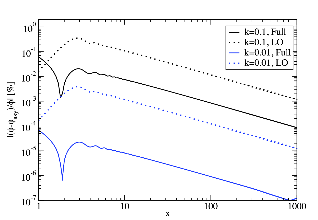
The left panel of Fig. 1 shows the difference between the numerical solution for and the asymptotic expansion in (46) to all computed orders in (solid line) and to linear order in (dotted lines). In all plots we have chosen to be that found in Sec. II.1.1. As expected, the solid lines are much closer to zero than the dotted ones. Moreover, notice that the asymptotic solutions found in the limit are already quite good (better than relative to the numerical solution) below .
The right-panel of Fig. 1 shows the same type of difference as the left-panel, but for the phase solution. As before, observe that the full solution agrees with the numerical solution much better than its truncated version. Unlike the solution, the is globally valid, as we did not restrict attention to the limit, and this can be clearly seen in Fig. 1. It is also apparent that, as expected, in both cases the smaller is, the better the asymptotic solution.
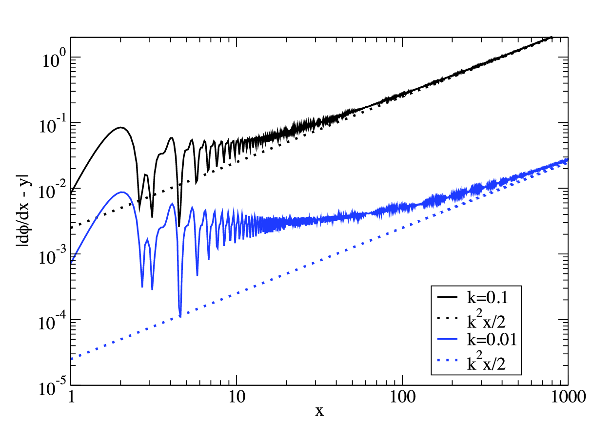
Although the previous figures establish that the asymptotic solutions are indeed accurate representations of the numerical ones, they do not compare the and solutions to each other. Figure 2 shows the difference between and computed numerically in both cases. As predicted by the asymptotic solutions, the difference is approximately (the dotted lines) in the limit.
IV Asymptotic transition at
As described in the previous sections, both the and solutions experience a transition as . In this section we discuss this transition in more detail using hyper-asymptotic tools.
IV.1 Frequency Resonances
Let us try to understand the fundamental change in the asymptotic behavior of the solution as transitions from to from above. To do so, we must find the most important term as approaches to all orders in powers of . Then, we must sum the series and identify the singularity at .
Assuming that , we know that the behavior of in (4) as is described by a series in inverse odd powers of :
| (64) |
where
| (65) |
As discussed earlier, as , , and thus approaches . To higher order in , one easily finds that
| (66) | |||||
| (67) |
Thus, when is small, the most singular part of is
| (68) |
Similarly, the most singular part of is
| (69) |
The numerical coefficients, , , , , , are given by a very simple formula:
| (70) |
Therefore, if we sum the most singular terms as to all orders in powers of , we find that
| (71) |
From the Taylor expansion
| (72) |
one finds that
| (73) |
where we have used the identity . This shows that there is a square-root-branch-cut singularity where the asymptotic behavior goes complex as .
In addition to this branch-cut singularity, one can also show that the higher-order terms in bunch up into families as , with each pair of families separated by an unstable separatrix curve. As shown earlier, as , the leading-order slope of the solution and approaches . There are, however, many solutions for in (65) as : the first lies just below (but above ); the second lies just above ; the third and fourth lie just below and just above , and so on.
Consider two different solutions, and corresponding to one of the infinite number of possible values of and define
| (74) |
Observe that satisfies the differential equation
| (75) |
Using the identity
| (76) |
we can rewrite (75) as
| (77) |
for large .
Let us now make the assumption that and approach one another as gets large, so that is small when . Then, this differential equation becomes
| (78) |
whose solution is
| (79) |
Note that this solution is growing exponentially if is positive, and thus the assumption that is small as is not valid. This is the unstable (separatrix) case. However, if is negative, then we have the stable case, and we have shown that the family of solutions corresponding to this case all bunch together exponentially fast. Note that there is an alternation between stable and unstable behavior: Stable behavior occurs only for the values of that are just below for , that is, , , , and so on, while unstable behavior occurs for the values of just above .
IV.2 Phase Resonances


The phase solutions also show a fundamental qualitative change of behavior as transitions from to . Because the phase differential equation, (5), admits a first integral of the motion, the analysis is simpler than in the frequency case and it does not require a hyper-asymptotic analysis. This is best understood if we consider the first-order form of (5), which we rewrite here as
| (80) |
where and . The potential is shown for representative values of in the left panel of Figure 3. Motion can only exist in regions where . The initial conditions correspond to . For , the effective potential has no turning points and for any initial conditions the motion will be unbounded with . When , the potential does have turning points. The right panel of Figure 3 shows a close-up of the potential for in the vicinity of the turning points. For , the motion is unbounded as in the case. However, for , the motion intersects the potential twice, and it can be oscillatory for suitable initial values of , or unbounded if is sufficiently large. For , the motion is again only unbounded for sufficiently large .
These specifications for and place restrictions on the initial conditions, which are inconsistent with the conditions we want to impose. For the conditions , the motion is unbounded for , the critical value computed in (32). When , the potential intersects the axis a second time. The motion will asymptotically approach the limiting value . For , the motion is oscillatory. At the next limiting solution for , , the effective potential has another intersection with the axis. However, this region is inaccessible to motion with these initial conditions and the motion is still oscillatory. Starting the motion with and would generate a solution that asymptotically approaches the next limiting value .
At the threshold value , two solutions , with will oscillate with different frequencies, and we therefore expect the difference to be oscillatory. If , one solution will be unbounded and therefore the difference will grow like . For , both solutions are unbounded, and we expect the difference to grow linearly with .
V Generalized Resonances
Section I derived certain equations [Eqs. (4) and (5)] that are representative of phase and frequency resonances in EMRIs, but in doing so we made two important simplifying assumptions: (b) we ignored the sine term in the sum given in Eq. (3) and (c) we ignored higher- terms in this same sum. In this section we relax these two assumptions and discuss how the solutions are modified.
Let us first relax assumption (b). If the sine term is included, (4) and (5) can be written as
| (81) |
where is a constant. We can repeat the analysis of the frequency evolution equation with the modification introduced above by making the ansatz
| (82) |
in place of (15). The analysis proceeds exactly as before, but with the arguments of the various cosine and sine terms modified via . The asymptotic slope, , is unchanged as a function of . The solution for will be modified, however, because the expansion for described in Sec. II.1.1 is modified. In particular
| (83) |
in which denotes the Fresnel sine function, defined by a similar equation to Eq. (13), but with the cosine replace by a sine. After asymptotic matching, we then find that .
In the phase-resonance case, the addition of the to the equation of motion is equivalent to solving the original problem with a modified initial condition: and . However, the solution to the modified equation with the standard initial condition can also be found straightforwardly using the method described in this paper. In that case, the zeroth-order-in- solution is unchanged, , but the first-order-in- correction, , is modified to
| (84) | |||||
from which we see that the asymptotic correction to the gradient is modified to . Continuing to the next order in , we obtain for the asymptotic gradient
| (85) |
for . We note that the leading-order-in- correction to the asymptotic gradient in the phase equation and the leading-order correction to in the frequency equation can be made to vanish for . However, even with this choice, the next-to-leading-order correction does not vanish, and so although the effect of the resonance can be suppressed for certain values of , it cannot be eliminated.
Let us now relax assumption (c); that is, let us include higher modes in the resonant differential equations. Consider first an evolution equation of the form
| (86) |
where is some integer. By writing , , we can rewrite this equation as
| (87) |
reducing it to the same form that we considered before. We note in particular that since the solution to this equation behaves as for , this implies that and hence the value of is unchanged as a function of . The value of would be modified, however.
In the phase case, if we modify the equation to
| (88) |
with again an integer, the substitution , gives
| (89) |
Using the solution to this equation that we found earlier, we find that and we deduce that
| (90) |
Clearly then, higher- modes in the sum of (3) are suppressed by a factor of .
Let us now consider the case where we have more than one term on the righthand side of the evolution equation. In the frequency resonance case, we would have an equation like
| (91) |
To solve this equation, we can proceed as before, making an ansatz of the form
| (92) |
Inserting this into the differential equation, we find the same source terms involving that we found earlier, one from each mode. We also find various cross source terms, but these do not contribute to the zero-frequency part of the solution because they are products of oscillatory functions with unequal frequencies. We deduce then that the solution for at leading order is the sum of the solutions treating each of the modes individually. At the next order, cross terms will come in that may be important, but these will be subdominant and further exploration of these is beyond the scope of this paper.
In the case of the phase equation we would have
| (93) |
The linear-in- term in the solution of this equation can readily be seen to be the sum of the linear-in- solutions to the equation with only one of the cosine terms on the righthand side. Cross terms again come in at higher order, but by the preceding argument the size of the corrections from the term are suppressed relative to the dominant mode by factors of .
VI Conclusions
We have studied the behavior of the solution to two differential equations that describe the gravitational-wave phase and frequency evolution during an EMRI that experiences a resonant transition. We have found two general differential equations that might describe this behavior: one based on the assumption that the coefficients of a Fourier expansion of the self-force in frequency are continuous at a resonance, and the other based on the assumption that it is the Fourier phase coefficients that are continuous at resonance. We have solved both differential equations at late times using asymptotic methods.
Depending on the strength of the resonance (controlled by the parameter ), both resonant equations lead to solutions with qualitative different behavior: Weak resonances () lead to linear temporal growth of the frequency and quadratic growth of the orbital phase; strong resonances () lead to linear temporal decay of the frequency function, leading to a constant-phase offset at late times.
Even though the differential equations for phase and frequency resonances might both describe the evolution of an EMRI through a resonance, we have found that the evolution depends on which differential equation one assumes. That is, at late times and in the weak resonance case, the evolution of the frequency in the phase and frequency resonant cases possess different asymptotic slopes. The difference in slope depends on the value of , with the frequency evolution acquiring a -dependent memory in the frequency resonant case that is absent for phase resonances. Further work is required to explore which of the two equations is in fact most applicable to the EMRI resonance problem.
We also studied the transition between weak and strong resonances. We found that at the transition point , there is a square-root branch cut in the solution to the frequency resonance equation. Close to this point, we proved that frequency solutions bunch up into families that decay as exponentially fast. In fact, there is an alternation between stable (bunching up of solutions) and unstable behavior, depending on the branch of solutions considered.
Future work should concentrate on exploring which of these equations is applicable to EMRI evolutions in practice and what the implications are for the construction of waveform template models of EMRI signals. The existence of a memory effect in the frequency resonances is particularly interesting and would have a profound impact on our ability to detect EMRI signals. An approximate post-Newtonian prescription for the self-force on resonance has been suggested [6] and would provide a suitable framework in which to explore these questions further. Whichever of the two equations applies to the problem that motivated this work, the results described in this paper provide important insights into the behaviour of the solutions to these differential equations and predictions for the change in the frequency and phase of the evolution as the orbit passes through a resonance. These results will be invaluable for constructing approximate models to describe the evolution of EMRI orbits.
Acknowledgements.
CMB is supported by grants from the Leverhulme Foundation and the U.S. Department of Energy. JG’s work is supported by the Royal Society. NY acknowledges support from NASA grant NNX11AI49G, under sub-award 00001944 and NASA through the Einstein Postdoctoral Fellowship Award Number PF0-110080 issued by the Chandra X-ray Observatory Center, which is operated by the Smithsonian Astrophysical Observatory for and on behalf of NASA under contract NAS8-03060. JG thanks the MIT Kavli Institute for Astrophysics and NY thanks the Yukawa Institute for Theoretical Physics for their hospitality while this paper was being finished. We also thank Scott Hughes for useful discussions.References
- [1] J. P. Boyd, Acta Applicandae 56, 1 (1999).
- [2] C. M. Bender and S. A. Orszag, Advanced mathematical methods for scientists and engineers 1, Asymptotic methods and perturbation theory (Springer, New York, 1999).
- [3] N. Yunes and E. Berti, Phys. Rev. D77, 124006 (2008), arXiv:0803.1853 [gr-qc] .
- [4] Z. Zhang, N. Yunes, and E. Berti, Phys.Rev. D84, 024029 (2011).
- [5] E. Berti, V. Cardoso, and A. O. Starinets, Class.Quant.Grav. 26, 163001 (2009), arXiv:0905.2975 [gr-qc] .
- [6] E. E. Flanagan and T. Hinderer, (2010), arXiv:1009.4923 [gr-qc] .
- [7] J. R. Gair, E. E. Flanagan, S. Drasco, T. Hinderer, and S. Babak, Phys.Rev. D83, 044037 (2011).
- [8] P. Amaro-Seoane et al., Class. Quantum Grav. 24, 113 (2007).
- [9] E. Poisson, Phys. Rev. D47, 1497 (1993).
- [10] S. A. Hughes, Phys. Rev. D61, 084004 (2000).
- [11] S. A. Hughes, Phys. Rev. D64, 064004 (2001).
- [12] A. Pound and E. Poisson, Phys. Rev. D77, 044013 (2008).
- [13] C. M. Bender, D. W. Hook, P. N. Meisinger, and Q.-h. Wang, Phys.Rev.Lett. 104, 061601 (2010a).
- [14] C. M. Bender, D. W. Hook, P. N. Meisinger, and Q.-h. Wang, Annals Phys. 325, 2332 (2010b).