Classical Motion in Random Potentials

Andreas Knauf ^†^†thanks: Department Mathematik, Universität Erlangen-Nürnberg, Cauerstr.˜11, D–91 058 Erlangen, Germany. e-mail: knauf@mi.uni-erlangen.de Christoph Schumacher ^†^†thanks: Fakultät für Mathematik, Technische Universität Chemnitz, Reichenhainerstr.˜$41$, D–09 126 Chemnitz, Germany. e-mail: christoph.schumacher@mathematik.tu-chemnitz.de

October 2011

Abstract

We consider the motion of a classical particle under the influence of a random potential on ${\mathbb{R}}^{d}$ , in particular the distribution of asymptotic velocities and the question of ergodicity of time evolution.

1 Introduction

Since its introduction to physics by Einstein and its mathematical foundation by Wiener, Brownian motion is considered one cornerstone of probability and of thermodynamics. It thus may seem natural to expect that classical motion in a spatially homogeneous force field leads in the large time limit to deterministic diffusion.

Such results can in fact be proven for a periodic Lorentz gas with finite horizon (related to the Sinai billiard) or for coulombic periodic potentials, see [BS81] respectively [Kna87, DL91].

However, in both cases the dynamics is non–smooth, of billiard type for the Lorentz gas and with orbits locally approximating Keplerian conic sections for the second case. We show here (Theorem 8.4), that the motion in a bounded smooth potential is incompatible with uniform hyperbolicity.

If periodic scatterers can lead to diffusive motion, the more this should be true for random scatterers. However, this is certainly not the case for 1D and also wrong for more degrees of freedom and Poisson potentials (Sections 6 and 7). In this and other cases the Hamiltonian flow is not even ergodic (Theorem 7.1).

For the random Coulomb case, however, we show in Theorem 9.5 that the flow is typically topologically transitive for large energies.

Related results on the motion in random configurations of convex scatterers have been derived by Marco Lenci and collaborators. In [Len03], the planar situation with a finite modification of periodic scatterers was studied. In [CLS10] (see also the references of that article) recurrence for particles in quenched tubes with random scatterers has been proven.

The literature on the corresponding quantum problem of Schrödinger operators with random potentials is much broader. See e.g., [LMW03], and [Ves08] with its extensive references.

In the article [RF11] quantum diffusion in a thermal medium has been proven.

We describe the structure of the paper. Random potentials arise in different guises. The one studied most extensively is based on a regular lattice ${\mathcal{L}}$ in configuration space. If $J$ indexes the single site potentials, on assumes a measure on the space $J^{\mathcal{L}}$ , for which the ${\mathcal{L}}$ –action is ergodic. This is studied in Section 2. One result is an almost deterministic distribution of asymptotic velocities (Section 3). One problem concerning the Liouville measure on the energy surface is discussed in Section 5. Depending on the exact exponential decay rate, the set of singular energy values may or may not be typically dense. Poissonian random potentials are studied in Sections 4 and 7. Relationships between different notions of ergodicity and some of their dynamical implications are discussed in Section 6. Section 8 concerns deterministic potentials, and the geometry compatible with a uniformly hyperbolic structure. Finally, we treat random coulombic potentials in Sections 9 and 10, showing topological transitivity and ergodicity of the compactified flow for energy surfaces of large energy.

Acknowledgement: We thank Boris Gutkin for the useful conversations.

2 The Lattice Case

We assume the random potential to be based on short range single site potentials $W_{j}\in C^{\eta}({\mathbb{R}}^{d},{\mathbb{R}})$ , indexed by $j\in J$ , $\lvert J\rvert\in{\mathbb{N}}$ , $\lvert J\rvert\geq 2$ . Namely $\eta\in{\mathbb{N}}\cup\{\infty\}$ , $\eta\geq 2$ and

\lvert\partial^{\alpha}W_{j}(q)\rvert\leq\frac{C_{\alpha}}{\left\langle q\right\rangle^{d+\varepsilon}}\qquad\bigl(q\in{\mathbb{R}}^{d},\ \alpha\in{\mathbb{N}}_{0}^{d},\ \lvert\alpha\rvert\leq\eta\bigr)

(2.1)

with $\left\langle q\right\rangle:=\sqrt{1+\lVert q\rVert^{2}}$ , for constants $C_{\alpha}>0$ .

The single site potentials are placed on a regular lattice ${\mathcal{L}}\subseteq{\mathbb{R}}^{d}$ with basis $\ell_{1},\dotsc,\ell_{d}\in{\mathbb{R}}^{d}$ according to $\omega\in\Omega:=J^{\mathcal{L}}$ to give the random potential

V\colon M:=\Omega\times{\mathbb{R}}^{d}\to{\mathbb{R}}\quad\text{,}\quad V(\omega,q):=\sum_{\ell\in{\mathcal{L}}}W_{\omega(\ell)}(q-\ell)

on extended configuration space $M$ . We use the discrete topology on $J$ and product topology on $\Omega$ . The probability measure $\beta$ on $\bigl(\Omega,{\cal B}(\Omega)\bigr)$ is assumed to be invariant w.r.t. the action

\vartheta\colon{\mathcal{L}}\times\Omega\to\Omega\quad\text{,}\quad(\ell,\omega)\mapsto\vartheta_{\ell}(\omega)\quad\text{with}\quad\vartheta_{\ell}(\omega)(\ell^{\prime}):=\omega(\ell^{\prime}+\ell)\text{.}

(2.2)

Unless we explicitly say the contrary, $\beta$ is assumed to be $\vartheta$ –ergodic (a simple example being a product measure $\beta=\bigotimes_{\ell\in{\mathcal{L}}}\hat{\beta}$ with a probability measure $\hat{\beta}$ on $J$ ). Ergodicity and $\lvert J\rvert\geq 2$ imply that $\beta$ is non–atomic. The short range conditions above imply that for all $\omega\in\Omega$ the potentials

V_{\omega}\colon{\mathbb{R}}^{d}\to{\mathbb{R}}\quad\text{,}\quad V_{\omega}(q):=V(\omega,q)

are as smooth as the single site potentials $W_{j}$ . Moreover $V$ itself is continuous and bounded, together with its partial derivatives $\partial^{\alpha}V,\ \lvert\alpha\rvert\leq\eta$ .

Remark 2.1.

More relevant than the range

[V_{\min},V_{\max}]:=\overline{V(M)}

of the potential is its essential range ( $\lambda^{d}$ denoting Lebesgue measure on ${\mathbb{R}}^{d}$ ):

\mathrm{supp}\bigl(V(\beta\otimes\lambda^{d})\bigr)=[V_{\operatorname{ess}\min},V_{\operatorname{ess}\max}]\text{.}

By $\vartheta$ –ergodicity of $\beta$ , this is a deterministic set:

\mathrm{supp}\bigl(V_{\omega}(\lambda^{d})\bigr)=\mathrm{supp}\bigl(V(\beta\otimes\lambda^{d})\bigr)\qquad(\beta\text{--a.s.})\text{.}

As $V$ is uniformly bounded together with its first derivatives, this is in fact a bounded interval: $\mathrm{supp}\bigl(V_{\omega}(\lambda^{d})\bigr)=\overline{V_{\omega}({\mathbb{R}}^{d})}$ . In general the essential range of $V$ is a proper subinterval of its range.

Thus the flow $\Phi\colon{\mathbb{R}}\times P\to P$ generated by the Hamiltonian function

H\colon P\to{\mathbb{R}}\quad\text{,}\quad H(\omega,p,q):={\textstyle\frac{1}{2}}\lVert p\rVert^{2}+V(\omega,q)

on extended phase space

P:=\Omega\times{\mathbb{R}}^{d}\times{\mathbb{R}}^{d}

uniquely exists for all times. We write

\Phi^{t}\colon P\to P\text{ , }\Phi^{t}(\omega,p_{0},q_{0}):=\Phi(t,\omega,p_{0},q_{0})=\left(\omega\,,\,p^{t}(\omega,p_{0},q_{0})\,,\,q^{t}(\omega,p_{0},q_{0})\right)

for the solution of the initial value problem at time $t\in{\mathbb{R}}$ . Whenever a fixed $\omega\in\Omega$ is considered, we write it as a subscript (e.g. $\Phi_{\omega}^{t}\equiv(p_{\omega}^{t},q_{\omega}^{t})\colon{\mathbb{R}}^{2d}\to{\mathbb{R}}^{2d})$ . See Figure 1 for a realisation of $t\mapsto q_{\omega}(t,x_{0})$ , with lattice ${\mathcal{L}}={\mathbb{Z}}^{2}$ .

Figure 1: Path in configuration space

The space $P$ is equipped with the locally finite Borel measure $\mu:=\beta\otimes\lambda^{2d}$ . The Hamiltonian flow $\Phi$ leaves $\mu$ invariant.

The lattice acts on extended phase space via the continuous group action

\Theta\colon{\mathcal{L}}\times P\to P\quad\text{,}\quad(\ell,\omega,p,q)\,\mapsto\,\Theta_{\ell}(\omega,p,q):=\bigl(\vartheta_{\ell}(\omega),p,q-\ell\bigr)

and leaves $\mu$ invariant:

\mu\circ\Theta_{\ell}=\mu\qquad(\ell\in{\mathcal{L}})\text{.}

(2.3)

Similarly for all lattice vectors $\ell\in{\mathcal{L}}$

H\circ\Theta_{\ell}=H\quad\text{and thus}\quad\Theta_{\ell}\circ\Phi^{t}=\Phi^{t}\circ\Theta_{\ell}\qquad(t\in{\mathbb{R}})\text{.}

(2.4)

By the Hamiltonian character of the motion the energy is invariant under the time evolution:

H\circ\Phi^{t}=H\qquad(t\in{\mathbb{R}})\text{.}

(2.5)

Thus we obtain a one–parameter family of Borel measures $\mu_{E}$ on $P$ , given by

\mu_{E}(B):=\mu\left(B\cap H^{-1}(-\infty,E])\right)\qquad\bigl(B\in{\cal B}(P)\bigr)\text{,}

(2.6)

parametrised by the energy $E\in{\mathbb{R}}$ . By (2.3), (2.4) and (2.5) these measures $\mu_{E}$ are $\Theta$ – and $\Phi$ –invariant, too.

A relevant quantity is asymptotic velocity

{\overline{v}}^{\pm}\colon P\to{\mathbb{R}}^{d}\quad\text{,}\quad{\overline{v}}^{\pm}(\omega,x_{0}):=\lim_{T\to\pm\infty}\frac{q_{\omega}(T,x_{0})}{T}\text{.}

(2.7)

Remark 2.2 (Non–Existence of Asymptotic Velocity).

For Hamiltonian motion in bounded potentials the asymptotic velocity may not exist for any initial condition $x_{0}\in H^{-1}(E)$ for all energies $E$ above some threshold. This is the case for centrally symmetric potentials ( $V(q)=\tilde{V}(\lVert q\rVert)$ ), with $\tilde{V}$ being periodic in a slowly varying function like, for example, $\tilde{V}(r)=\cos(\log(r+1))$ .

It is also possible to construct examples of truly random potentials where for some $\omega\in\Omega$ these limits do not exist on $H_{\omega}^{-1}(E)$ for any $E>E_{0}$ :

The lattice ${\mathcal{L}}:={\mathbb{Z}}^{d}$ with fundamental domain ${\cal D}=[0,1]^{d}$ admits an adapted partition of unity $F_{\ell}$ , $(\ell\in{\mathcal{L}})$

{\textstyle\sum_{\ell\in{\mathcal{L}}}}F_{\ell}(q)=1\qquad(q\in{\mathbb{R}}^{d})

with $F_{\ell}(q):=F(q-\ell)$ for $F:={\rm 1\mskip-4.0mul}_{\cal D}\,*\,f$ with some $f\in C_{c}^{\infty}\bigl({\mathbb{R}}^{d},[0,\infty)\bigr)$ and $\int_{{\mathbb{R}}^{d}}f\,dx=1$ .

We now take $J:=\{0,1,\ldots,d\}$ as index set for the single site potentials $W_{j}:=j\,F$ . We choose $\omega\in\Omega=J^{({\mathbb{Z}}^{d})}$ of the form $\omega(\ell)=\sum_{k=1}^{d}\widetilde{\omega}_{k}(\ell_{k})$ , with $\widetilde{\omega}_{k}:{\mathbb{Z}}\to\{0,1\}$ slowly varying like above.

Then the motion in the realization $V_{\omega}$ is separable in cartesian coordinates, and thus for no $E>E_{0}:=d$ and initial condition $x_{0}\in H_{\omega}^{-1}(E)$ the asymptotic velocities ${\overline{v}}^{\pm}(x_{0})$ exist.

By allowing for arbitrary modifications of $\omega$ over finite subsets of ${\mathbb{Z}}^{d}$ the set of these $\widehat{\omega}$ is even dense in $\Omega$ , and asymptotic velocity does not exist for any initial condition $x_{0}\in H_{\widehat{\omega}}^{-1}(E)$ (possibly except for dimension $d>1$ and a set of finite Liouville measure, for which ${\overline{v}}^{\pm}(\widehat{\omega},x_{0})=0$ ).

In case of non–existence of the limit, we will set ${\overline{v}}^{\pm}(\omega,x_{0}):=0$ .

However, typically the above limit exists. This is shown below by invoking Birkhoff’s ergodic theorem. As this deals with finite measures, we have to change our measure space. Namely, we set

\hat{P}:=P/\Theta\text{.}

As $P=\bigcup_{\ell\in{\mathcal{L}}}\Theta_{\ell}(\Omega\times{\mathbb{R}}^{d}_{p}\times{\cal D})$ with fundamental domain of ${\mathcal{L}}$

{\cal D}\,:=\,\bigl\{{\textstyle\sum_{k=1}^{d}}x_{k}\ell_{k}\ \bigm|\ x_{k}\in[0,1]\bigr\}\,\subseteq\,{\mathbb{R}}^{d}_{q}\text{,}

the topological space $\hat{P}$ is homeomorphic to

(\Omega\times{\mathbb{R}}^{d}\times{\cal D})/{\sim}\text{,}

(2.8)

$\sim$ identifying points in $\Omega\times{\mathbb{R}}^{d}_{p}\times\partial{\cal D}$ via the $\Theta$ action. Using (2.3) and (2.4), the covering projection

\hat{\pi}\colon P\to\hat{P}

allows us to induce measures ${\hat{\mu}}$ and ${\hat{\mu}}_{E}$ on $\hat{P}$ by setting

{\hat{\mu}}({\hat{B}}):=\mu\bigl(\hat{\pi}^{-1}({\hat{B}})\cap(\Omega\times{\mathbb{R}}^{d}_{p}\times{\cal D})\bigr)\qquad\bigl({\hat{B}}\in{\cal B}({\hat{P}})\bigr)

(2.9)

and similarly for ${\hat{\mu}}_{E}$ (note that the Lebesgue measure $\lambda^{d}(\partial{\cal D})=0$ ).

Furthermore (2.4) allows us to define the continuous energy function ${\hat{H}}\colon{\hat{P}}\to{\mathbb{R}}$ and flow ${\hat{\Phi}}\colon{\mathbb{R}}\times{\hat{P}}\to{\hat{P}}$ uniquely by $H={\hat{H}}\circ\hat{\pi}$ and ${\hat{\Phi}}^{t}\circ\hat{\pi}=\hat{\pi}\circ\Phi^{t}$ . Finally, by $\Theta$ –invariance of the momenta $p\colon P\to{\mathbb{R}}^{d}$ , they descend to

{\hat{p}}\colon{\hat{P}}\to{\mathbb{R}}^{d}\quad\text{,}\quad{\hat{p}}\circ\hat{\pi}=p.

(2.10)

Proposition 2.3.

The asymptotic velocities (2.7) exist $\mu$ –a.e. on $P$ , and ${\overline{v}}^{+}={\overline{v}}^{-}\ \mu$ –a.e. . Setting ${\overline{v}}(x):={\overline{v}}^{\pm}(x)$ in case of equality and ${\overline{v}}(x)=0$ otherwise,

{\overline{v}}\in L_{\mathrm{loc}}^{\infty}(P,\mu)\quad\text{,}\quad{\overline{v}}\circ\Phi^{t}={\overline{v}}\quad\text{and}\quad{\overline{v}}\circ\Theta_{\ell}={\overline{v}}\qquad(t\in{\mathbb{R}},\ell\in{\mathcal{L}})\text{.}

Proof:

For initial conditions $x_{0}=(p_{0},q_{0})\in{\mathbb{R}}^{d}_{p}\times{\mathbb{R}}^{d}_{q}$ we have

	$\displaystyle{\overline{v}}^{\pm}(\omega,x_{0})$	$\displaystyle=\lim_{T\to\pm\infty}\frac{q_{\omega}(T,x_{0})-q_{0}}{T}=\lim_{T\to\pm\infty}\frac{1}{T}\int_{0}^{T}p_{\omega}(t,x_{0})\,dt$
		$\displaystyle=\lim_{T\to\pm\infty}\frac{1}{T}\int_{0}^{T}{\hat{p}}\bigl(t,\hat{\pi}(\omega,x_{0})\bigr)\,dt\text{.}$

But as the finite measures ${\hat{\mu}}_{E}$ on ${\hat{P}}$ are ${\hat{\Phi}}$ –invariant, by Birkhoff’s ergodic theorem the limits $\lim_{T\to\pm\infty}\frac{1}{T}\int_{0}^{T}{\hat{p}}(t,\hat{x}_{0})\,dt$ exist, coincide and are ${\hat{\Phi}}$ –invariant ${\hat{\mu}}_{E}$ –a.e. . Moreover the limit function lies in $L^{1}({\hat{P}},{\hat{\mu}}_{E})$ and is bounded by $\sqrt{2(E-V_{\min})}$ in absolute value, as $\lVert{\hat{p}}(t,\hat{x}_{0})\rVert^{2}\leq 2({\hat{H}}(\hat{x}_{0})-V_{\min})$ . Thus it is in $L^{\infty}({\hat{P}},{\hat{\mu}}_{E})$ .

The measure ${\hat{\mu}}$ is non–finite, but ${\hat{\mu}}{\upharpoonright}_{{\hat{H}}^{-1}((-\infty,E])}={\hat{\mu}}_{E}$ . Thus we obtain the result. $\Box$

Corollary 2.4.

For $\beta$ –a.e. $\omega\in\Omega$ the asymptotic velocities ${\overline{v}}_{\omega}^{\pm}\colon{\mathbb{R}}^{d}_{p}\times{\mathbb{R}}^{d}_{q}\to{\mathbb{R}}^{d}$ exist and are equal $\lambda^{2d}$ –a.e. .

Proof:

This follows from Proposition 2.3 and Fubini’s theorem, applied to the measure $\mu=\beta\otimes\lambda^{2d}$ on extended phase space $P$ . $\Box$

Similarly, for all regular energies $E$ (see Section 6 below), the asymptotic velocities exist Liouville–almost everywhere on $H^{-1}_{\omega}(E)$ .

3 Distribution of Asymptotic Velocities

Next we consider the joint distribution of energy and asymptotic velocity, using the measurable maps

\Gamma_{\omega}:=(H_{\omega},{\overline{v}}_{\omega})\colon{\mathbb{R}}^{d}_{p}\times{\mathbb{R}}^{d}_{q}\longrightarrow{\mathbb{R}}\times{\mathbb{R}}^{d}\qquad(\omega\in\Omega)\text{.}

We thus consider phase space regions ${\mathbb{R}}^{d}_{p}\times Q_{n}\subseteq{\mathbb{R}}^{d}_{p}\times{\mathbb{R}}^{d}_{q}$ with

Q_{n}:=\bigl\{{\textstyle\sum_{k=1}^{d}}x_{k}\ell_{k}\ \bigm|\ \forall k\in\{1,\dotsc,d\}:\;-n\leq x_{k}<n\bigr\}\qquad(n\in{\mathbb{N}})\text{,}

and the normalised restrictions

\lambda_{n}\,:=\,\frac{1}{\lambda^{d}(Q_{n})}\lambda^{2d}{\upharpoonright}_{{\mathbb{R}}^{d}_{p}\times Q_{n}}\,=\,(2n)^{-2d}\;\lambda^{2d}{\upharpoonright}_{{\mathbb{R}}^{d}_{p}\times Q_{n}}

of Lebesgue measure to these regions.

Proposition 3.1.

For $\beta$ –a.e. $\omega\in\Omega$ the energy velocity distribution

\nu_{\omega}:=\lim_{n\to\infty}\Gamma_{\omega}(\lambda_{n})

exists in the sense of vague convergence and is independent of $\omega$ .

Proof:

In view of Riesz representation theorem we have to check that for every function $f\in C_{c}({\mathbb{R}}^{d+1})=\{g\in C({\mathbb{R}}^{d+1})\mid\mathrm{supp}(g)\text{ is compact}\}$

\lim_{n\to\infty}\int_{{\mathbb{R}}^{d+1}}f\,d\nu_{n,\omega}\qquad\text{, with $\nu_{n,\omega}:=\Gamma_{\omega}(\lambda_{n})$,}

exists and is independent of $\omega$ . By compactness of support of $f$ , there exists an $E_{0}\in{\mathbb{R}}$ (depending on $f$ ) with $f(E,{\overline{v}})=0$ for all ${\overline{v}}\in{\mathbb{R}}^{d}$ and $E\geq E_{0}$ . On the other hand we know that $\lVert p\rVert\leq\sqrt{2(E_{0}-V_{\min})}$ if $(p,q)\in H^{-1}([V_{\min},E_{0}])$ . Thus we have the estimate

\int_{{\mathbb{R}}^{d+1}}\lvert f\rvert\,d\nu_{n,\omega}\leq\frac{(2(E_{0}-V_{\min})\,\pi)^{d/2}}{\Gamma\left(\frac{d}{2}+1\right)}\cdot\lVert f\rVert_{\infty}\text{,}

which is uniform in $n\in{\mathbb{N}}$ and $\omega\in\Omega$ . The function

g\colon\Omega\to{\mathbb{R}}\quad\text{,}\quad g(\omega):=\int_{{\mathbb{R}}^{d+1}}f\,d\nu_{1,\omega}

is thus in $L^{\infty}(\Omega,\beta)$ . Moreover

\int_{{\mathbb{R}}^{d+1}}f\,d\nu_{n,\omega}=\frac{1}{\lvert{\mathcal{L}}_{n}\rvert}\sum_{\ell\in{\mathcal{L}}_{n}}g\bigl(\vartheta_{\ell}(\omega)\bigr)

with ${\mathcal{L}}_{n}:=\bigl\{\sum_{k=1}^{d}n_{k}\ell_{k}\mid n_{k}\in\{-n,-n+1,\ldots,n-1\}\bigr\}\subseteq{\mathcal{L}}$ .

By assumption the probability measure $\beta$ is ergodic w.r.t. the $\vartheta$ –action on $\Omega$ . Thus a lattice version of Birkhoff’s ergodic theorem (see, e.g. Keller [Kel98], Thm. 2.1.5) assures that

\lim_{n\to\infty}\int_{{\mathbb{R}}^{d+1}}f\,d\nu_{n,\omega}\ \text{ exists\ and\ is\ $\omega$--independent}

$\beta$ –almost surely. $\Box$

The energy–velocity distribution is the unique non–random limit measure

\hat{\nu}\colon{\cal B}({\mathbb{R}}^{d+1})\to[0,\infty]\text{.}

This measure always has a certain symmetry property:

Proposition 3.2.

The energy–velocity distribution $\hat{\nu}$ is invariant w.r.t. the inversion of velocity

I\colon{\mathbb{R}}^{d+1}\to{\mathbb{R}}^{d+1}\quad\text{,}\quad(E,{\overline{v}})\mapsto(E,-{\overline{v}})\text{.}

Proof:

Consider $\omega\in\Omega$ with $\nu_{\omega}=\hat{\nu}$ and ${\overline{v}}_{\omega}^{+}(p_{0},q_{0})={\overline{v}}_{\omega}^{-}(p_{0},q_{0})$ for $\lambda^{2d}$ –a.e. phase space point $(p_{0},q_{0})\in{\mathbb{R}}^{2d}$ . (By Propositions 3.1 and 2.4 $\beta$ –a.e. $\omega$ meets these conditions.)

By reversibility of the flow $\Phi_{\omega}^{t}=(p_{\omega}^{t},q_{\omega}^{t})$ , that is

p_{\omega}^{t}(-p_{0},q_{0})=-p_{\omega}^{-t}(p_{0},q_{0})\quad\text{,}\quad q_{\omega}^{t}(-p_{0},q_{0})=q^{-t}_{\omega}(p_{0},q_{0})\,\text{,}

we have ${\overline{v}}_{\omega}^{+}(-p_{0},q_{0})=-{\overline{v}}_{\omega}^{-}(p_{0},q_{0})$ . Together this gives

{\overline{v}}_{\omega}(-p_{0},q_{0})=-{\overline{v}}_{\omega}(p_{0},q_{0})\qquad(\lambda^{2d}\text{--a.e.})\text{.}

On the other hand the phase space region ${\mathbb{R}}^{d}\times Q_{n}$ as well as the measure $\lambda_{n}$ on it are invariant w.r.t. the antisymplectic transformation $(p,q)\mapsto(-p,q)$ on phase space. Thus the image measures $\nu_{n,\omega}=\Gamma_{\omega}(\lambda_{n})$ are $I$ –invariant. This carries over to the vague limit $\nu_{\omega}=\hat{\nu}$ . $\Box$

Definition 3.3.

For $\omega\in\Omega$ a phase space point $x_{0}=(p_{0},q_{0})\in{\mathbb{R}}^{2d}$ is called forward resp. backward bounded if

q_{\omega}\bigl([0,\infty),x_{0}\bigr)\quad\text{resp.}\quad q_{\omega}\bigl((-\infty,0],x_{0}\bigr)

are bounded subsets of configuration space ${\mathbb{R}}^{d}$ .

Note that $\lambda^{2d}$ –a.e. $x_{0}\in{\mathbb{R}}^{2d}$ is simultaneously bounded or unbounded in both time directions. This is a direct consequence of the flow invariance of $\lambda^{2d}$ .

Proposition 3.4.

For $E>V_{\operatorname{ess}\max}$ and for $\beta$ –a.e. $\omega\in\Omega$ for every initial position $q_{0}\in{\mathbb{R}}^{d}$ there exists an initial direction $p_{0}\in{\mathbb{R}}^{d}$ with $H_{\omega}(p_{0},q_{0})=E$ and $(p_{0},q_{0})$ forward unbounded, with positive minimal speed ( $\inf_{t>0}\lVert(q(t)-q_{0})/t\rVert>0$ ).

Proof:

For $\beta$ -a.a. $\omega\in\Omega$ we have $V_{\omega}(q)\leq V_{\operatorname{ess}\max}$ for all $q\in{\mathbb{R}}^{d}$ (see Remark 2.1 and use the continuity of $V_{\omega}$ ). Thus the Jacobi metric $g_{E,\omega}$ on configuration space ${\mathbb{R}}^{d}$ , given by

g_{E,\omega}(q)=\bigl(E-V_{\omega}(q)\bigr)g_{\mathrm{Euclid}}\text{,}

(3.1)

is non–degenerate, and the riemannian manifold $({\mathbb{R}}^{d},g_{E,\omega})$ is geodesically complete, since the conformal factor is bounded below by $E-V_{\operatorname{ess}\max}>0$ . So the Hopf–Rinow theorem (see, e.g., [GHL48], Thm. 2.103) implies for any $q_{n}\in{\mathbb{R}}^{d}$ the existence of an initial direction $v_{n}\in S_{q_{0}}:=\{v\in{\mathbb{R}}^{d}\mid g_{E,\omega}(q_{0})(v,v)=1\}$ such that the forward geodesic $t\mapsto\gamma(t,q_{0},v_{n})$ with initial condition $(q_{0},v_{n})$ meets $q_{n}$ first at a time $t_{n}\geq 0$ , and is a shortest such geodesic so that

\lVert\gamma(t,q_{0},v_{n})-q_{0}\rVert\geq\sqrt{2(E-V_{\operatorname{ess}\max})}\,t\qquad\bigl(n\in{\mathbb{N}},\ t\in[0,t_{n}]\bigr)\text{.}

For $\lim_{n\rightarrow\infty}\lVert q_{n}-q_{0}\rVert=\infty$ , $\lim_{n\rightarrow\infty}t_{n}=+\infty$ , and by compactness of $S_{q_{0}}$ there is an accumulation point $v_{\infty}\in S_{q_{0}}$ of the $v_{n}$ leading to forward unbounded geodesic motion.

Up to parametrisation, the geodesic of $g_{E,\omega}$ with initial condition $(q_{0},v_{\infty})$ coincides with the trajectory $q_{\omega}(t,x_{0})$ (with $x_{0}:=\bigl(2\bigl(E-V_{\omega}(q_{0})\bigr)\,v_{\infty},q_{0}\bigr)$ as initial condition), see [AM78, Thm. 3.7.7]. The positivity of the minimal speed is preserved. $\Box$

In dimensions $d\geq 2$ bounded and unbounded motion can coexist $\beta$ –a.s. for energies $E>V_{\operatorname{ess}\max}$ as well as for $E<V_{\operatorname{ess}\max}$ . In one dimension this is not possible:

Proposition 3.5.

For $d=1$ and $\beta$ –a.e. $\omega\in\Omega$ the motion through $x_{0}=(p_{0},q_{0})$ is bounded if $E:=H_{\omega}(x_{0})<V_{\operatorname{ess}\max}$ and unbounded with asymptotic velocity

{\overline{v}}_{\omega}(x_{0})=\frac{\ell_{1}}{{\mathbb{E}}_{\beta}\bigl(\tau(x_{0})\bigr)}\quad\text{,}\quad\tau_{\omega}(x_{0})=\int_{0}^{\ell_{1}}\frac{\mathrm{sign}(p_{0})}{\sqrt{2(E-V_{\omega}(q))}}\,dq

if $E>V_{\operatorname{ess}\max}$ .

Remark 3.6.

Here the asymptotic velocity depends on $(\omega,x_{0})\in P$ only via $H_{\omega}(x_{0})$ and $\mathrm{sign}(p_{0})$ . Figure 2 shows the shape of $\mathrm{supp}(\hat{\nu})\subseteq{\mathbb{R}}^{2}$ .

Figure 2: Shape of

\mathrm{supp}(\hat{\nu})\subseteq{\mathbb{R}}^{2}

Proof:

$\bullet$

For $E<V_{\operatorname{ess}\max}$ the connected component of $x_{0}$ in $H_{\omega}^{-1}(E)$ is compact $\beta$ –a.s., since there exist $q^{\pm}\in{\mathbb{R}}$ with $V_{\omega}(q^{\pm})>E$ and $q^{-}<q_{0}<q^{+}$ .

\bullet

For $E>V_{\operatorname{ess}\max}$ the asymptotic velocity, if it exists for $x_{0}$ , equals

{\overline{v}}(\omega,x_{0})=\lim_{T\to\infty}\frac{1}{T}\int_{0}^{T}p_{\omega}(t,x_{0})\,dt=\lim_{n\to\infty}\frac{\int_{0}^{T_{n}(\omega)}p_{\omega}(t,x_{0})\,dt}{T_{n}(\omega)}

with $T_{n}(\omega)$ for $n\in{\mathbb{N}}$ determined uniquely by $q_{\omega}(T_{n}(\omega),x_{0})-q_{0}=n\ell_{1}$ . Here we assume w.l.o.g. $\ell_{1}>0$ and $p_{0}>0$ . The numerator equals

\int_{0}^{T_{n}(\omega)}\dot{q}_{\omega}(t,x_{0})\,dt=q_{\omega}(T_{n}(\omega),x_{0})-q_{0}=n\ell_{1}\text{,}

whereas

T_{n}(\omega)=\sum_{k=0}^{n-1}\int_{q_{0}+k\ell_{1}}^{q_{0}+(k+1)\ell_{1}}\frac{1}{\sqrt{2(E-V_{\omega}(q))}}\,dq

for the denominator. Setting

g\colon\Omega\to{\mathbb{R}}\quad\text{,}\quad g(\omega):=\int_{q_{0}}^{q_{0}+\ell_{1}}\frac{1}{\sqrt{2(E-V_{\omega}(q))}}\,dq\text{,}

we get $T_{n}(\omega)=\sum_{k=0}^{n-1}$ $g\bigl(\vartheta_{k\ell_{1}}(\omega)\bigr)$ . By continuity of $g$ , we can apply Birkhoff’s theorem and get by the ergodicity assumption on $\beta$

\lim_{n\to\infty}\frac{1}{n}T_{n}(\omega)=\lim_{n\to\infty}\frac{1}{n}\sum_{k=0}^{n-1}g\bigl(\vartheta_{k\ell_{1}}(\omega)\bigr)={\mathbb{E}}(g)\qquad\text{$\beta$--a.s.}\text{.}

This proves the assertion for $\lambda^{2}$ –a.e. $x_{0}\in{\mathbb{R}}^{2}$ with $H_{\omega}(x_{0})>V_{\operatorname{ess}\max}$ . The expression $\frac{1}{T}\int_{0}^{T}p_{\omega}(t,p_{0},q_{0})\,dt$ is monotonically increasing in $p_{0}$ , and our formula for ${\overline{v}}_{\omega}(x_{0})$ is continuous in $p_{0}$ . Thus it must be valid for all $x_{0}$ .

$\Box$

For $d\geq 2$ it is an interesting question whether for large energies the asymptotic velocity distribution given by $\hat{\nu}$ is zero. As the example below shows, this is not always the case for non–trivial random potentials.

Example 3.7 (Random Potential With Non-Zero Asymptotic Velocity).

We use the cutoff function $F\in C_{c}^{\infty}({\mathbb{R}}^{d},[0,1])$ from Remark 2.2 for the lattice ${\mathcal{L}}:={\mathbb{Z}}^{d}$ . Given single site potentials ${\hat{W}}_{j}$ with $\mathrm{supp}({\hat{W}}_{j})\subseteq\left[\frac{1}{4},\frac{3}{4}\right]^{d}$ , we set $W_{j}(q):={\hat{W}}_{j}(q)-\sum_{k=1}^{d}\cos(2\pi q_{k})F(q)$ . Then the random potential equals

V_{\omega}(q)\;=\;{\textstyle\sum_{\ell\in{\mathcal{L}}}}W_{\omega(\ell)}(q-\ell)\;=\;{\hat{V}}_{\omega}(q)-{\textstyle\sum_{k=1}^{d}}\cos(2\pi q_{k})

with ${\hat{V}}_{\omega}(q):=\sum_{\ell\in{\mathcal{L}}}{\hat{W}}_{\omega(\ell)}(q-\ell)$ .

Thus the Hamiltonian function $H_{\omega}\colon{\mathbb{R}}^{d}\times{\mathbb{R}}^{d}\to{\mathbb{R}}$ takes the form

H_{\omega}(p,q)={\hat{V}}_{\omega}(q)+{\textstyle\sum_{k=1}^{d}}H_{\omega}^{(k)}(p_{k},q_{k})

with $H_{\omega}^{(k)}\colon{\mathbb{R}}^{d}\to{\mathbb{R}},\ (p_{k},q_{k})\mapsto\frac{1}{2}p_{k}^{2}-\cos(2\pi q_{k})$ . The phase space regions

P_{k}:=\bigl\{(p,q)\in{\mathbb{R}}^{d}\times({\mathbb{R}}^{d}\setminus S)\mid\forall\,m\in\{1,\ldots,d\}\setminus\{k\}:H_{\omega}^{(m)}(p_{m},q_{m})<0\bigl\}

with $S:={\mathcal{L}}+\left[{\textstyle\frac{1}{4}},{\textstyle\frac{3}{4}}\right]^{d}$ are invariant w.r.t. $\Phi_{\omega}^{t}$ , since ${\hat{V}}_{\omega}(q)=0$ for $q\in{\mathbb{R}}^{d}\setminus S$ , and thus the motion separates.

For all $x=(p,q)\in P_{k}$ the asymptotic velocity exists. If in addition $E:=H_{\omega}^{(k)}(p_{k},q_{k})>1$ , then ${\overline{v}}^{\pm}(x)=(0,\ldots,0,{\overline{v}}^{(k)},0,\dotsc,0)$ with ${\overline{v}}^{(k)}:=\frac{\mathrm{sign}(p_{k})\pi\sqrt{E-1}}{\sqrt{2}{\cal K}(2/(1-E))}$ , ${\cal K}$ being the complete elliptic integral of the first kind (see [AK98]).

As $E\nearrow\infty$ , the intersections $P_{k}\cap H_{\omega}^{-1}(E)$ have density w.r.t. Liouville measure on $H_{\omega}^{-1}(E)$ scaling like $E^{-(d-1)/2}$ .

Thus for no total energy strictly above $2-d$ the distribution of asymptotic velocity is concentrated in zero.

4 Poisson Potentials

Compared to the lattice case handled above, potentials based on marked Poisson fields have some new features like unboundedness and invariance w.r.t. ${\mathbb{R}}^{d}$ –translations. So we discuss them in this section. Many properties should generalise to other ergodic random potentials (like gaussian potentials).

Again we start with single site potentials $W_{j}$ indexed by $j\in J$ , $\lvert J\rvert<\infty$ , but we assume for simplicity that for some $\eta\geq 2$

W_{j}\in C_{c}^{\eta}({\mathbb{R}}^{d},{\mathbb{R}})\text{.}

We now consider the marked Poisson process with space

	$\displaystyle\tilde{\Omega}:=\bigl\{\omega\bigm\|\omega$	measure on $\bigl({\mathbb{R}}^{d}\times J,\ {\cal B}({\mathbb{R}}^{d}\times J)\bigr)$ with
		$\displaystyle\omega(K)\in{\mathbb{N}}_{0}\text{ if $K\subseteq{\mathbb{R}}^{d}\times J$ is compact}\bigr\}\text{.}$

$\tilde{\Omega}$ is the space of all counting measures on ${\mathbb{R}}^{d}\times J$ and carries the vague topology generated by the basis consisting of the sets

\hskip-5.69054pt{\cal N}_{\omega}(\psi_{0},\dotsc,\psi_{k}):=\bigl\{\omega^{\prime}\in\tilde{\Omega}\bigm|\forall i\in\{0,\dotsc,k\}\colon\lvert\textstyle\int\psi_{i}\,d\omega^{\prime}-\int\psi_{i}\,d\omega\rvert<1\bigr\}

(4.1)

with $k\in{\mathbb{N}}_{0}$ , $\omega\in\tilde{\Omega}$ and $\psi_{i}\in C_{c}({\mathbb{R}}^{d}\times J,{\mathbb{R}})$ ( $i\in\{0,\dotsc,k\}$ ), see, e.g. [Rue87]. For $j\in J$ and compact $K\in{\cal B}({\mathbb{R}}^{d})$ the random variables

N_{K,j}\colon\tilde{\Omega}\to{\mathbb{N}}_{0}\quad\text{,}\quad\omega\mapsto\omega(K\times\{j\})\text{,}

are called particle number functions. We fix intensities $\rho_{j}{}\geq 0,\ j\in J$ . Then $\beta$ is the unique probability measure on $\bigl(\tilde{\Omega},{\cal B}(\tilde{\Omega})\bigr)$ with

\beta\bigl(\{\omega\in\tilde{\Omega}\mid N_{K,j}(\omega)=m\}\bigr)=\frac{\bigl(\rho_{j}\lambda^{d}(K)\bigr)^{m}}{m!\exp\bigl(\rho_{j}\lambda^{d}(K)\bigr)}

(4.2)

for all $m\in{\mathbb{N}}_{0}$ , $j\in J$ and $K\in{\cal B}({\mathbb{R}}^{d})$ with $\lambda^{d}(K)<\infty$ .

$\bigl({\mathbb{R}}^{d}\times J,\tilde{\Omega},{\cal B}(\tilde{\Omega}),\beta\bigr)$ is called marked Poisson process on ${\mathbb{R}}^{d}$ with marks in $J$ and intensities $\rho_{j}$ , see [SKM87, Chap. 4.2]. It induces the random potential

V\colon\tilde{M}:=\tilde{\Omega}\times{\mathbb{R}}^{d}\longrightarrow{\mathbb{R}}\quad\text{,}\quad(\omega,q)\longmapsto\int_{{\mathbb{R}}^{d}\times J}W_{j}(q-x)\,d\omega(x,j)\text{.}

Proposition 4.1.

The potential $V\colon\tilde{\Omega}\to{\mathbb{R}}$ is continuous, and

V_{\omega}\in C^{\eta}({\mathbb{R}}^{d},{\mathbb{R}})\qquad(\omega\in\tilde{\Omega})\text{.}

There is a $\beta$ –measure zero subset $N\subseteq\tilde{\Omega}$ such that for $\Omega:=\tilde{\Omega}\setminus N$ and extended phase space $P:=\Omega\times{\mathbb{R}}^{d}\times{\mathbb{R}}^{d}$ the restriction $H:=\tilde{H}{\upharpoonright}_{P}$ of the Hamiltonian function

\tilde{H}\colon\tilde{P}\to{\mathbb{R}}\quad\text{,}\quad(\omega,p,q)\mapsto{\textstyle\frac{1}{2}}\lVert p\rVert^{2}+V(\omega,q)

induces a continuous Hamiltonian flow

\Phi\colon{\mathbb{R}}\times P\to P\text{.}

Proof:

\bullet

To show continuity of $V$ , we construct for $\varepsilon>0$ a neighbourhood

U(\omega,q)\,:=\,{\cal N}_{\omega}(\psi_{1},\ldots,\psi_{k})\times B_{\delta}(q)\,\subseteq\,\tilde{M}\,=\,\tilde{\Omega}\times{\mathbb{R}}^{d}

of $(\omega,q){}\in\tilde{\Omega}\times{\mathbb{R}}^{d}$ , such that $\lvert V(\omega^{\prime},q^{\prime})-V(\omega,q)\rvert<\varepsilon$ for all $(\omega^{\prime},q^{\prime})\in U(\omega,q)$ . For radius $R:=\sup\{\lVert x\rVert\mid x\in\bigcup_{j\in J}\mathrm{supp}(W_{j})\}+1$ only the finitely many Poisson points in

{{\cal S}_{R,q}}:=\mathrm{supp}(\omega)\cap(B_{R}(q)\times J)\equiv\{(q_{1},j_{1}),\ldots,(q_{k},j_{k})\}

can contribute to $V(\omega,q)$ , and their minimal distance

d_{\min}:=\inf\{\lVert q_{m}-q_{n}\rVert\mid 1\leq m,n\leq k,q_{m}\neq q_{n}\}

is positive. We will need the loci ${\cal S}_{R,q}^{j}(\omega)$ of the support of $\omega$ with index $j\in J$ , implicitely given by

{{\cal S}_{R,q}}=\bigcup_{j\in J}{\cal S}_{R,q}^{j}(\omega)\times\{j\}\text{,}

and a common Lipschitz constant $L$ for the single site potentials $(W_{j})_{j\in J}$ .

With $\delta:=\min\bigl\{\frac{\varepsilon}{2L\,\omega({\cal S}_{R,q})},\frac{d_{\min}}{3},1\bigr\}>0$ we choose $A_{j}:=B_{R}(q)\setminus B_{\delta}({\cal S}_{R,q}^{j}(\omega))$ and, employing the Kronecker delta $\delta_{\cdot,\cdot}$ and the positive part $(\cdot)_{+}:=\max\{0,\cdot\}$ , functions $\psi_{i}\in C_{c}({\mathbb{R}}^{d}\times J,{\mathbb{R}})$ with

\psi_{i}(x,j):=\begin{cases}\bigl(1-\mathrm{dist\,}(x,A_{j})/\delta\bigr)_{+}&(i=0)\\ \bigl(1-\delta_{j,j_{i}}\mathrm{dist\,}(x,B_{\delta}(q_{i}))/\delta\bigr)_{+}&(i\in\{1,\ldots,k\})\end{cases}

Thus $\int_{{{\mathbb{R}}^{d}}}\psi_{i}\,d\omega=(1-\delta_{0,l})\omega\{(q_{i},j_{i})\}$ , and by definition (4.1) of ${\cal N}_{\omega}(\psi_{0},\ldots,\psi_{k})$ , all $(\omega^{\prime},q^{\prime})\in U(\omega,q)$ fulfil the relations

\lVert q^{\prime}-q\rVert\leq\delta\quad\text{,}\quad\omega^{\prime}(A_{j}\times\{j\})=0\quad\text{and}\quad\omega^{\prime}(B_{\delta}(q_{i})\times\{j_{i}\})=\omega\{(q_{i},j_{i})\}\text{,}

$j\in J$ . With this preparation we deduce

		$\displaystyle\lvert V(\omega^{\prime},q^{\prime})-V(\omega,q)\rvert$
		$\displaystyle\leq\sum_{j\in J}\Bigl\|\Bigl(\sum_{\tilde{q}\in{\cal S}_{R,q}^{j}(\omega^{\prime})}W_{j}(q^{\prime}-\tilde{q})\omega^{\prime}(\tilde{q},j)\Bigr)-\sum_{\hat{q}\in{\cal S}_{R,q}^{j}(\omega)}W_{j}(q-\hat{q})\omega(\hat{q},j)\Bigr\|$
		$\displaystyle\leq\sum_{j\in J}\sum_{\hat{q}\in{\cal S}_{R,q}^{j}(\omega)}\Bigl\|\Bigl(\sum_{\tilde{q}\in{\cal S}_{\delta,\hat{q}}^{j}(\omega^{\prime})}W_{j}(q^{\prime}-\tilde{q})\omega^{\prime}(\tilde{q},j)\Bigr)-W_{j}(q-\hat{q})\omega(\hat{q},j)\Bigr\|$
		$\displaystyle\leq\sum_{j\in J}\sum_{\hat{q}\in{\cal S}_{R,q}^{j}(\omega)}\sum_{\tilde{q}\in{\cal S}_{\delta,\hat{q}}^{j}(\omega^{\prime})}\lvert W_{j}(q^{\prime}-\tilde{q})-W_{j}(q-\hat{q})\rvert\omega^{\prime}(\tilde{q},j)$
		$\displaystyle\leq\sum_{j\in J}\sum_{\hat{q}\in{\cal S}_{R,q}^{j}(\omega)}2L\delta\,\omega(\hat{q},j)=2L\delta\,\omega({\cal S}_{R,q})\leq\varepsilon\text{,}$

since $\lVert q^{\prime}-\tilde{q}-(q-\hat{q})\rVert\leq\lVert q^{\prime}-q\rVert+\lVert\tilde{q}-\hat{q}\rVert\leq 2\delta$ .

\bullet

This implies that $\tilde{H}\colon\tilde{P}\to{\mathbb{R}}$ , too, is continuous on $\tilde{P}:=\tilde{\Omega}\times{\mathbb{R}}^{2d}$ and for all $\omega\in\tilde{\Omega}$ the Hamiltonian $\tilde{H}_{\omega}\in C^{\eta}({\mathbb{R}}^{2d},{\mathbb{R}})$ . However, this only guarantees local unique existence of the flow. We now set

N:=\bigl\{\omega\in\tilde{\Omega}\bigm|\liminf_{\lVert q\rVert\to\infty}V_{\omega}(q)+c\left\langle q\right\rangle^{2}=-\infty\ \text{for\ all}\ c>0\bigr\}

(4.3)

For $\omega\in\tilde{\Omega}\setminus N$ and $E\in{\mathbb{R}}$ there exists a $C>0$ with

\sqrt{2(E-V_{\omega}(q))_{+}}\leq C\left\langle q\right\rangle\qquad(q\in{\mathbb{R}}^{d})\text{.}

Thus the solution of the initial value problem with energy $E$ exists for all times. Namely as

\left\langle q_{\omega}(t)\right\rangle\frac{d}{dt}\left\langle q_{\omega}(t)\right\rangle\leq\lVert q_{\omega}(t)\rVert\,\lVert p_{\omega}(t)\rVert\leq C\left\langle q_{\omega}(t)\right\rangle^{2}\text{,}

$t\mapsto\lVert q_{\omega}(t)\rVert$ is at most of exponential growth.

$\bullet$

We show that $\beta(N)=0$ . We set $W_{\max}:=\max\{\lvert W_{j}(q)\rvert\mid(q,j)\in{\mathbb{R}}^{d}\times J\}>0$ , ${\rm diam}:=\max_{j}{\rm diam\,}({\rm supp\,}W_{j})$ and $N_{B_{r}(q),J}:=\sum_{j\in J}N_{B_{r}(q),j}$ . $\beta(N)=0$ follows from $\lim_{R\to\infty}\beta(N_{R})=0$ with

$N_{R}:=\bigl\{\omega\in\tilde{\Omega}\bigm|\min_{\lVert q\rVert\leq R}V_{\omega}(q)\leq-R^{2}\bigr\}\text{.}$ (4.4)

Now for $V_{\omega}(q)\leq-R^{2}$ to occur for any point $q\in B_{\rm diam}(Q)$ we must have

$N_{B_{2{\rm diam}(Q)},J}(\omega)\geq R^{2}/W_{\max}.$ (4.5)

As $B_{R}(0)$ is ${\rm diam}$ –spanned (see Walters [Wal82]) by a set ${\cal Q}\subseteq B_{R}(0)$ of points $Q$ with cardinality $\lvert{\cal Q}\rvert={\cal O}(R^{d})$ , (4.4) follows from (4.5) and (4.2).
$\bullet$

Finally, continuity of the flow $\Phi$ follows from the theorem on continuous dependence of solutions on parameters.

$\Box$

Remark 4.2 (Comparison With Quantum Mechanics).

We have

{\mathbb{E}}_{\beta}\left(\lvert V_{\centerdot}(0)\rvert^{\frac{d+\varepsilon}{2}}\right)\leq(W_{\max})^{\frac{d+\varepsilon}{2}}\,{\mathbb{E}}_{\beta}(N_{B_{R}(0),J})^{\frac{d+\varepsilon}{2}}

(4.6)

Estimate (4.6) should be compared with a criterion for essential self-adjointness of the corresponding random Schrödinger operator $-\Delta+V$ on $L^{2}({\mathbb{R}}^{d})$ . This is generally true for $\vartheta$ –ergodic $V$ if ${\mathbb{E}}_{\beta}\bigl(\lvert V(0)\rvert^{\tilde{d}}\bigr)<\infty$ for $\tilde{d}:=2\lceil\frac{d+1}{4}\rceil$ , see [PF92], Theorem 5.1.

Unlike in the lattice case the Poisson potential $V$ is invariant w.r.t. a faithful ${\mathbb{R}}^{d}$ –action on $P$ : For $\ell\in{\mathbb{R}}^{d}$ set

\vartheta_{\ell}\colon\tilde{\Omega}\to\tilde{\Omega}\quad\text{,}\quad\vartheta_{\ell}(\omega)(A):=\omega(\{(\ell+x,j)\mid(x,j)\in A\})\text{.}

(4.7)

Then $N$ , defined in (4.3), is $\vartheta$ –invariant so that we get the ${\mathbb{R}}^{d}$ action

\Theta\colon{\mathbb{R}}^{d}\times P\to P\quad\text{,}\quad(\ell,\omega,p,q)\mapsto(\vartheta_{\ell}(\omega),p,q-\ell)

on extended phase space, with

H\circ\Theta_{\ell}=H\quad\text{,}\quad\mu\circ\Theta_{\ell}=\mu\quad\text{and}\quad\Phi^{t}\circ\Theta_{\ell}=\Theta_{\ell}\circ\Phi^{t}

for all $t\in{\mathbb{R}}^{d}$ and $\ell\in{\mathbb{R}}^{d}$ .

In order to control the existence of the asymptotic velocities, we select an arbitrary regular lattice ${\mathcal{L}}\subseteq{\mathbb{R}}^{d}$ , e.g. ${\mathcal{L}}:={\mathbb{Z}}^{d}$ , and set $\Theta^{\mathcal{L}}:=\Theta{\upharpoonright}_{{\mathcal{L}}\times P}$ .

Then, as in Section 2 above, we consider the covering projection

\hat{\pi}\colon P\to\hat{P}:=P/\Theta^{\mathcal{L}}

to the factor space ${\hat{P}}$ . Like in (2.8), ${\hat{P}}$ is homeomorphic to $(\Omega\times{\mathbb{R}}^{d}\times{\cal D})/{\sim}$ .

On ${\hat{P}}$ we consider the measures ${\hat{\mu}}$ and ${\hat{\mu}}_{E}\ (E\in{\mathbb{R}})$ , defined like in (2.9).

Again, by $\Theta$ –invariance similar to (2.10) we can define momenta on ${\hat{P}}$ by

{\hat{p}}\colon{\hat{P}}\to{\mathbb{R}}^{d}\quad\text{,}\quad{\hat{p}}\circ{\hat{\pi}}=p\text{.}

But unlike in Section 2, the potential $V_{\omega}$ is $\beta$ –a.s. unbounded, and thus ${\hat{H}}^{-1}((-\infty,E])$ is compact only if the $W_{j}$ are non–negative. Therefore we need the following lemma:

Lemma 4.3.

For all $E\in{\mathbb{R}}$ the measure ${\hat{\mu}}_{E}$ on ${\hat{P}}$ is finite, and

\int_{\hat{P}}\lVert{\hat{p}}\rVert\,d{\hat{\mu}}_{E}<\infty.

(4.8)

Proof:

We estimate, setting $r(q):=\sqrt{2(E-V(q))_{+}}$ ,

{\hat{\mu}}_{E}({\hat{P}})={\mathbb{E}}_{\beta}\left(\int_{{\cal D}}\int_{{\mathbb{R}}^{d}}{\rm 1\mskip-4.0mul}_{B_{r(q)}}(p)\,dp\,dq\right)=\tau_{d}\,\lambda^{d}({\cal D})\,{\mathbb{E}}_{\beta}\left(2\bigl(E-V(0)\bigr)_{+}^{\ d/2}\right)<\infty

with $\tau_{d}:=\lambda^{d}\bigl(B_{1}(0)\bigr)=\frac{\pi^{d/2}}{\Gamma(1+d/2)}$ , and similar (but with exponent $(d+1)/2$ ) for (4.8). $\Box$

Thus we get the analog of Proposition 2.3:

Proposition 4.4.

The asymptotic velocities ${\overline{v}}^{\pm}(\omega,x_{0})\,:=\,\lim_{T\to\pm\infty}\frac{q_{\omega}(T,x_{0})}{T}$ exist and are equal $\beta$ –a.s. on $P$ . Furthermore

{\overline{v}}\in L^{\infty}_{\mathrm{loc}}(P)\quad\text{and}\quad{\overline{v}}\circ\Phi^{t}={\overline{v}}\circ\Theta_{\ell}={\overline{v}}\text{.}

Proof:

We invoke Birkhoff’s theorem for

{\overline{v}}^{\pm}(\omega,x_{0})=\lim_{T\to\pm\infty}\frac{1}{T}\int_{0}^{T}{\hat{p}}\bigl(t,{\hat{\pi}}(\omega,x_{0})\bigr)\,dt\text{,}

using Lemma 4.3. $\Box$

Remarks 4.5.

1.

The ${\mathbb{R}}^{d}$ action (4.7) is mixing on $\tilde{\Omega}$ , see [PF92, p. 27]. Thereby the action of the lattice ${\mathcal{L}}$ by translations $\vartheta_{\ell}\ (\ell\in{\mathcal{L}})$ on $\tilde{\Omega}$ is mixing, too, and in particular $\beta$ –ergodic. Thus, like in Proposition 3.1, the energy–velocity distributions $\Gamma_{\omega}$ for the Poisson potentials are $\beta$ –a.s. deterministic.
2.

For $d=1$ one gets a result similar to Proposition 3.5. Note, however that $\mathrm{supp}\bigl(V(\beta\otimes\lambda^{d})\bigr)$ equals the closure of $(V_{\operatorname{ess}\min},\infty)$ , if there is a single site potential $W_{j}$ with $W_{j}(q)>0$ for some $q\in{\mathbb{R}}$ . In that case all motion is bounded $\beta$ –a.s. .

5 Singular Values of the Hamiltonian

Since Hamiltonian motion enjoys conservation of energy, one has to decompose phase space into energy shells in order to find ergodic motion. This is possible for regular energy values, so we first study the set of singular values of the Hamilton function. Both for the lattice and the Poisson case we have the following result:

Proposition 5.1.

The closure of the set of singular values of $V_{\omega}$ is $\beta$ –almost surely deterministic.

Proof:

For $S_{k,m}:=[m2^{-k},(m+1)2^{-k}]$ with $k\in{\mathbb{N}}$ and $m\in{\mathbb{Z}}$ the set

\Omega_{k,m}:=\bigl\{\omega\in\Omega\bigm|\exists q\in{\mathbb{R}}^{d}:\nabla_{q}V(\omega,q)=0\mbox{ and }V(\omega,q)\in S_{k,m}\bigr\}

is ${\mathcal{L}}$ -invariant. Thus by $\beta$ –ergodicity it is of measure zero or one. The sets $S_{k}:=\bigcup_{m\in{\mathbb{Z}}:\,\beta(\Omega_{k,m})=1}S_{k,m}$ are closed, and $S_{k+1}\subseteq S_{k}$ .

\Omega_{k}:=\{\omega\in\Omega\bigm|{\rm CVal}_{\omega}\subseteq S_{k}\}

is still invariant and of measure one. The same is true for $\Omega_{\infty}:=\bigcap_{k\in{\mathbb{N}}}\Omega_{k}$ . The potentials indexed by $\omega\in\Omega_{\infty}$ have their critical values in the closed set $S_{\infty}:=\bigcap_{k\in{\mathbb{N}}}S_{k}$ . It is $\beta$ –almost surely the closure of the set of singular values of $V_{\omega}$ . $\Box$

Example 5.2 (Denseness of Singular Values).

The set of singular values may be dense in $[V_{\operatorname{ess}\min},V_{\operatorname{ess}\max}]$ . This is the case $\beta$ –almost surely for the random ${\mathbb{Z}}$ –lattice potential on ${\mathbb{R}}$ given by the single site potentials

W_{j}(q):=\textstyle{\sum_{\ell\in{\mathbb{N}}}}\;j\lvert J\rvert^{-\ell}\chi\bigl(q-(-1)^{\ell}\lfloor\ell/2\rfloor\bigr)\quad\bigl(q\in{\mathbb{R}},\;j\in J:=\{0,\ldots,\lvert J\rvert-1\}\bigr)\text{,}

with $\chi\in C^{\infty}_{c}({\mathbb{R}},[0,1])$ , $\chi{\upharpoonright}_{\left[-{\textstyle\frac{1}{4}},{\textstyle\frac{1}{4}}\right]}=1$ and ${\rm supp}(\chi)\subseteq[-{\textstyle\frac{1}{2}},{\textstyle\frac{1}{2}}]$ , if $\beta:=\otimes_{{\mathbb{Z}}}\hat{\beta}$ is the product measure of $\hat{\beta}:=\textstyle{\sum_{j\in J}}\delta_{j}/\lvert J\rvert$ . Then for any $\omega\in\Omega=J^{\mathbb{Z}}$ with a dense $\vartheta$ –orbit the set of singular values is dense in $[0,1]$ and this is the case for $\beta$ -a.e. $\omega\in\Omega$ .

Note that the fall-off of the single site potentials is not only polynomial as assumed in (2.1) but exponential, with rate $W_{j}(q)={\cal O}\bigl(\lvert J\rvert^{-2|q|}\bigr)$ .

The exponential decay in this example is below the rate that ensures measure zero for the closure of the set ${\rm CVal}_{\omega}=V_{\omega}({\rm CSet}_{\omega})$ of singular values of $V_{\omega}$ :

Proposition 5.3.

Let for $d=1$ and some $\varepsilon>0$ the single site potentials $W_{j}\in C^{2}({\mathbb{R}},{\mathbb{R}})$ obey (for the lattice ${\mathbb{Z}}$ ) the decay estimate $W_{j}^{\prime}(q)={\cal O}\bigl(\lvert J\rvert^{-(4+\varepsilon)\lvert q\rvert}\bigr)$ . Then

\lambda^{1}\bigl(\overline{{\rm CVal}_{\omega}}\bigr)=0\qquad(\omega\in\Omega)\text{.}

Proof:

$\bullet$ By using the lattice translation $\vartheta$ , it suffices to show that

\lambda^{1}\left(\overline{{\textstyle\bigcup_{\omega\in\Omega}}V_{\omega}({\rm CSet}_{\omega}\cap[0,1])}\right)=0.

(5.1)

For this we prove that for $R\in{\mathbb{N}}$ large and the middle sequence $\omega^{(R)}\in J^{\{-R,\ldots,R\}}$ of $\omega$ we have

V_{\omega}\bigl({\rm CSet}_{\omega}\cap[0,1]\bigr)\;\subseteq\;M_{\omega^{(R)}}\qquad(\omega\in\Omega)\text{,}

(5.2)

for suitable closed subsets $M_{\tau}\subseteq{\mathbb{R}}$ of measures

\lambda^{1}(M_{\tau})\leq\lvert J\rvert^{-(2+\varepsilon/4)R}\qquad\bigl(\tau\in J^{\{-R,\ldots,R\}}\bigr)\text{.}

(5.3)

As this implies $\lambda^{1}\Bigl(\overline{{\textstyle\bigcup_{\omega\in\Omega}V_{\omega}({\rm CSet}_{\omega}\cap}[0,1])}\Bigr)\leq\lvert J\rvert^{1-\varepsilon R/4}$ , (5.1) then follows as $R\rightarrow\infty$ .
$\bullet$ $c^{(2)}:=\sup\bigl\{\sum_{j\in{\mathbb{Z}}}\lvert W^{\prime\prime}_{\omega_{j}}(q-j)\rvert\bigm|\omega\in\Omega,q\in{\mathbb{R}}\bigr\}<\infty$ is a uniform upper bound for the second derivative of

\tilde{V}_{\tau}(q):={\textstyle\sum_{\ell=-R}^{R}}W_{\tau(\ell)}(q-\ell)\qquad\bigl(q\in{\mathbb{R}},\,\tau\in J^{\{-R,\ldots,R\}}\bigr)\text{.}

Then for $\delta\leq c^{(2)}$ the disjoint union $\{x\in[0,1]\mid\lvert\tilde{V}^{\prime}_{\tau}(x)\rvert\leq\delta\}$ of closed intervals has at most $i_{\max}(\tau)\leq c^{(2)}/\delta$ intervals $I_{1}(\tau),\dotsc,I_{i_{\max}(\tau)}(\tau)$ containing a point $q$ with $\tilde{V}^{\prime}_{\tau}(q)=0$ , since each such interval has at least length $\delta/c^{(2)}$ .
We set $M_{\tau}:=\bigcup_{i=1}^{i_{\max}(\tau)}B_{\delta^{2}}\big(\tilde{V}_{\tau}(I_{i}(\tau))\big)$ . This union of thickened intervals has measure

\lambda^{1}(M_{\tau})\leq\lambda^{1}\Bigl(\tilde{V}_{\tau}\big({\bigcup\nolimits}_{i=1}^{i_{\max}(\tau)}I_{i}(\tau)\big)\Bigr)+2\delta^{2}\cdot i_{\max}(\tau)\leq(1+2c^{(2)})\;\delta\text{.}

So for $\delta\equiv\delta_{R}:=\lvert J\rvert^{-(2+\varepsilon/2)R}$ and $R$ large, (5.3) is satisfied.
$\bullet$ By the decay assumption $|W_{j}^{\prime}(q)|\leq c\lvert J\rvert^{-(4+\varepsilon)\lvert q\rvert}$ on the derivatives of the single site potentials, for $q\in[0,1]\setminus\bigcup_{i=1}^{i_{\max}(\tau)}I_{i}(\tau)$ one has

\lvert V^{\prime}_{\omega}(q)\rvert\geq\lvert\tilde{V}^{\prime}_{\tau}(q)\rvert-c\sum_{\ell\in{\mathbb{Z}}:|\ell|>R}\lvert J\rvert^{-(4+\varepsilon)\lvert\ell\rvert}\geq\delta_{R}-c\,\delta_{R}^{2}>0

for $R$ large enough. So ${\rm CSet}_{\omega}\cap[0,1]\subseteq\bigcup_{i=1}^{i_{\max}(\tau)}I_{i}(\tau)$ in (5.2).
$\bullet$ The single site potentials themselves, and not only their derivatives, decay like $W_{j}(q)={\cal O}\bigl(\lvert J\rvert^{-(4+\varepsilon)|q|}\bigr)$ . This means that

\lvert V_{\omega}(q)-\tilde{V}_{\omega^{(R)}}(q)\rvert\leq c\textstyle\sum_{\ell\in{\mathbb{Z}}:|\ell|>R}\lvert J\rvert^{-(4+\varepsilon)\lvert\ell\rvert}\leq\delta^{2}\qquad\big(q\in[0,1]\big).

But $\delta^{2}$ is the parameter appearing in the definition of $M_{\tau}$ . So (5.2) is satisfied, too. $\Box$

A similar statement, but with superexponential decay rate ${\cal O}\bigl(\lvert J\rvert^{-(c_{\mathcal{L}}+\varepsilon)\|q\|^{d}}\bigr)$ , should be sharp for $d\geq 1$ , with a constant $c_{\mathcal{L}}$ depending on the lattice ${\mathcal{L}}\subseteq{\mathbb{R}}^{d}$ .

We denote the restriction of the flow $\Phi_{\omega}$ to the energy surface $\Sigma_{E,\omega}:=H_{\omega}^{-1}(E)\subseteq{\mathbb{R}}^{2d}$ by $\Phi_{E,\omega}$ . For regular values $E$ of $H_{\omega}$ , $\Sigma_{E,\omega}$ carries a $\Phi_{E,\omega}$ –invariant measure $\lambda_{E,\omega}$ derived from Lebesgue measure $\lambda^{2d}$ on phase space (see, e.g. [AM78], Thm. 3.4.12).

This non–atomic Liouville measure thus exists for all $E>V_{\max}$ , using the equality of regular values of $H_{\omega}$ and $V_{\omega}$ .

For $V_{\omega}\in C^{d}({\mathbb{R}}^{d},{\mathbb{R}})$ by Sard’s theorem (see, e.g. [Hir76, Thm. 3.1.3]) it in fact exists for almost all energies $E>\inf V_{\omega}$ .

Remark 5.4 (Denseness of Singular Values, Poisson Case).

For (non–trivial) Poisson potentials, $\beta$ –almost surely, the set $\overline{{\rm CVal}_{\omega}}$ equals ${\mathbb{R}}$ , $[0,\infty)$ or $(-\infty,0]$ , depending on the signs occuring in the union of ranges of the single site potentials. This is true, since

(a)

for any real number $r$ between zero and an extreme value of $W_{j}$ the sum $U_{a}(q):=W_{j}(q)+W_{j}(q+ae_{1})$ of $W_{j}$ and its translate by a suitable $a={}a(r)\in{\mathbb{R}}$ has $r$ as a singular value. For the case $\max\;W_{j}=W_{j}(q_{0})>0$ we take

$\mathrm{MM}(a):=\sup_{c\in C}\min_{t\in[0,1]}U_{a}\bigl(c(t)\bigr)\text{,}$

with $C:=\bigl\{c\in C^{\infty}\bigl([0,1],{\mathbb{R}}^{d}\bigr)\bigm|c(0)=q_{0},c(1)=q_{0}+ae_{1}\bigr\}$ . Then $\mathrm{MM}(0)=2\max W_{j}$ , $\mathrm{MM}(a)=0$ for $\lvert a\rvert$ large, and $\mathrm{MM}$ is continuous. Furthermore $\mathrm{MM}(a)$ is a singular value for $U_{a}$ .

The case $\min W_{j}=W_{j}(q_{0})<0$ is treated by the reverse minmax problem.
(b)

Integer multiples of $W_{j}$ are Poisson potentials, too.

6 Notions of Ergodicity of Time Evolution

In general $\lambda_{E,\omega}$ is non–finite. Nevertheless, we may ask whether it is an ergodic measure (in the sense of Aaronson [Aar97]), that is, whether the only $\Phi_{\omega}$ –invariant measurable subsets $A\subseteq\Sigma_{E,\omega}$ have measure zero or full measure, i.e. $\lambda_{E,\omega}(\Sigma_{E,\omega}\setminus A)=0$ . Instead, we may also ask whether the restriction

{\hat{\Phi}}_{E}^{t}:={\hat{\Phi}}^{t}{{\upharpoonright}}_{\hat{\Sigma}_{E}}\ (t\in{\mathbb{R}})

(6.1)

of the flow ${\hat{\Phi}}$ to the (extended) energy surfaces $\hat{\Sigma}_{E}:={\hat{H}}^{-1}(E)\subseteq{\hat{P}}$ is ergodic. Here the Liouville measure ${\hat{\lambda}}_{E}$ on $\hat{\Sigma}_{E}$ , derived from the measure ${\hat{\mu}}$ on ${\hat{P}}$ by disintegration, is finite. Ergodicity of $\hat{\Phi}_{E}$ is much cheaper obtained than ergodicity of $\Phi_{E,\omega}$ , since on finite measure spaces Poincaré’s recurrence theorem holds, see Section 10. In this section we clarify the relations between the two notions of ergodicity and give some immediate consequences. The results pertain to both lattice and Poisson potentials (using quotients by ${\mathbb{Z}}^{d}$ in the latter case).

Proposition 6.1.

If for energy $E\in{\mathbb{R}}$ , the flow $\Phi_{E,\omega}$ on $\Sigma_{E,\omega}$ is $\lambda_{E,\omega}$ –ergodic for $\beta$ –a.e. $\omega\in\Omega$ , then the flow ${\hat{\Phi}}_{E}$ on $\Sigma_{E}$ is ${\hat{\mu}}_{E}$ –ergodic.

Proof:

Assume that $\hat{\Phi}_{E}$ is not ergodic. Then there exists a measurable invariant ( ${\hat{\lambda}}_{E}\bigl(\hat{A}\Delta{\hat{\Phi}}_{E}^{t}(\hat{A})\bigr)=0\ \text{for\ all}\ t\in{\mathbb{R}}$ ) subset $\hat{A}\subseteq\hat{\Sigma}_{E}$ with $0<{\hat{\lambda}}_{E}(\hat{A})<{\hat{\lambda}}_{E}(\hat{\Sigma}_{E})$ . Its pre-image $A:={\hat{\pi}}^{-1}(\hat{A})\subseteq\Sigma_{E}=H^{-1}(E)$ is measurable and invariant, too, w.r.t. the Liouville measure $\lambda_{E}$ on $\Sigma_{E}$ . Finally, $\lambda_{E}(A)>0$ and $\lambda_{E}(A^{c})>0$ , as $A^{c}=\Sigma_{E}\setminus A={\hat{\pi}}^{-1}\bigl(\hat{\Sigma}_{E}\setminus\hat{A}\bigr)$ .

So $A_{\omega}:=A\cap\Sigma_{E,\omega}$ is $\Phi_{E,\omega}$ –invariant $\beta$ –a.s., and similar for $A_{\omega}^{c}:=A^{c}\cap\Sigma_{E,\omega}=\Sigma_{E,\omega}\setminus A_{\omega}$ .

By $\vartheta$ –ergodicity of $\beta$ the $\beta$ -a.s. $\vartheta$ -invariant functions

f_{A},f_{A^{c}}\colon\Omega\to\{0,1\}\quad\text{,}\quad f_{A}(\omega)=\begin{cases}1&\text{,}\ \lambda_{E,\omega}(A_{\omega})>0\\ 0&\text{, otherwise}\end{cases}

(resp. for $A_{\omega}^{c}$ ) are both $\beta$ –a.s. constant with value $1$ . Thus $\Phi_{E,\omega}$ is not $\lambda_{E,\omega}$ –ergodic $\beta$ –a.s. . $\Box$

Note in passing that the flow $\Phi_{E}$ on $\Sigma_{E}$ is not $\lambda_{E}$ –ergodic (given $\beta$ is not a Dirac measure on $\Omega$ ), since $\Omega$ is unchanged by that flow.

Next we ask about the dynamical consequences of ergodicity.

Proposition 6.2.

Given $E\in{\mathbb{R}}$ and $\omega\in\Omega$ such that $\Phi_{E,\omega}$ is $\lambda_{E,\omega}$ –ergodic on the regular energy surface $\Sigma_{E,\omega}$ ,

•

then the asymptotic velocity ${\overline{v}}(x)=0$ for a.e. $x\in{}\Sigma_{E,\omega}$ ,
•

but the motion is unbounded a.e. on $\Sigma_{E,\omega}$ unless $\Sigma_{E,\omega}$ is compact.

Remark 6.3.

Note that $\Sigma_{E,\omega}$ is non–compact for $E>V_{\max}$ and $\beta$ –a.s. non–compact for $E>V_{\operatorname{ess}\min}$ , given ergodicity of $\Phi_{E,\omega}$ .

Proof:

Remember that ${\overline{v}}(x)=0$ by definition if ${\overline{v}}^{\pm}(x)$ do not exist or are unequal.

$\bullet$

Assume that $\lambda_{E,\omega}(\{x\in\Sigma_{E,\omega}\mid{\overline{v}}(x)\neq 0\})>0$ . Then there exists an open half space $H_{s}:=\{q\in{\mathbb{R}}^{d}\mid\left\langle q,s\right\rangle>0\}$ indexed by a unit vector $s\in S^{d-1}$ so that

$\lambda_{E,\omega}(B_{s})>0\quad\text{for}\quad B_{s}:=\{x\in\Sigma_{E,\omega}\mid{\overline{v}}(x)\in H_{s}\}\text{.}$

By reversibility of the flow and $\overline{v}^{-}=\overline{v}^{+}$

$\lambda_{E,\omega}(B_{-s})=\lambda_{E,\omega}(B_{s})\text{.}$

On the other hand, ${\overline{v}}\circ\Phi^{t}={\overline{v}}\quad(t\in{\mathbb{R}})$ , so that $B_{s}$ and $B_{-s}$ are disjoint invariant subsets of positive measure. Thus $\Phi_{E,\omega}$ is not $\lambda_{E,\omega}$ –ergodic.
$\bullet$

Assume that there exists a subset $B\subseteq\Sigma_{E,\omega}$ of points leading to forward bounded motion with $\lambda_{E,\omega}(B)>0$ . Then for some $r>0$ the subset

$B_{r}:=\{(p,q)\in B\mid\lVert q\rVert\leq r\}$

is of positive measure, too. Furthermore, for some $r^{\prime}>r$ the same applies to

$B_{r,r^{\prime}}:=\{x\in B_{r}\mid\lVert q_{t}(\omega,x)\rVert\leq r^{\prime}\text{ for\ all}\ t\geq 0\}\text{.}$

Finally the set

${\tilde{B}}:=\bigcup_{t\geq 0}\Phi_{E,\omega}^{t}(B_{r,r^{\prime}})\subseteq\Sigma_{E}$

is $\Phi_{E,\omega}$ –invariant w.r.t. $\lambda_{E,\omega}$ , and $\lambda_{E,\omega}({\tilde{B}})>0$ . But by non–compactness of $\Sigma_{E,\omega}$ , its complement ${\tilde{B}}^{c}=\Sigma_{E,\omega}\setminus{\tilde{B}}$ is of measure $\lambda_{E,\omega}({\tilde{B}}^{c})>0$ , since ${\tilde{B}}$ is bounded: $\lVert q\rVert\leq r^{\prime}$ if $(p,q)\in{\tilde{B}}$ . Thus $\Phi_{E,\omega}$ is not $\lambda_{E,\omega}$ –ergodic.

$\Box$

In one–dimensional natural mechanical systems with Hamiltonian $H\colon{\mathbb{R}}^{2}\to{\mathbb{R}},\ H(p,q)=\frac{1}{2}p^{2}+V(q)$ ergodicity on regular energy surfaces $\Sigma_{E}=H^{-1}(E)$ is widespread and occurs for compact as well as non–compact $\Sigma_{E}$ (examples: $V(q)=q^{2},\ V(q)=q$ ).

In our present context, however, ergodicity in one dimension is exceptional.

Proposition 6.4.

For $d=1$ and $E>V_{\operatorname{ess}\min}$ the flow $\Phi_{t,\omega}$ on a regular energy surface $\Sigma_{E,\omega}$ is $\beta$ –a.s. not $\lambda_{E,\omega}$ –ergodic.

Proof:

We assume that $\omega$ is chosen so that ${\overline{v}}^{+}(x)={\overline{v}}^{-}(x)$ for $\lambda_{E,\omega}$ –a.e. $x\in{\mathbb{R}}$ . This assumption is valid $\beta$ –a.s. . For $E<V_{\operatorname{ess}\max}$ the motion is bounded $\beta$ –a.s., whereas for $E>V_{\operatorname{ess}\max}$ asymptotic velocity is non–zero $\beta$ –a.s. according to Proposition 3.5.

Both statements contradict Proposition 6.2 (note that $\Sigma_{E,\omega}$ is non–compact $\beta$ –a.s. for $E>V_{\operatorname{ess}\min}$ ).

But for the case left, $E=V_{\operatorname{ess}\max},\ \Sigma_{E,\omega}$ must be connected, regular and non–compact. Thus it must be diffeomorphic to ${\mathbb{R}}$ . This can only occur if there is a $q_{0}$ so that $V(q)>E$ for all $q\in(q_{0},\infty)$ and $V(q)<E$ for all $q\in(-\infty,q_{0})$ or vice versa. This, however, would contradict our initial assumption ${\overline{v}}^{+}(x)={\overline{v}}^{-}(x)$ . $\Box$

Example 3.7 together with Proposition 6.2 shows that for any dimension $d$ there are non–trivial random lattice potentials that lead to non–ergodic motion on the regular energy surfaces $\Sigma_{E,\omega}$ for any $E$ and $\omega\in\Omega$ .

The statements of Proposition 6.2 can be proven under a different assumption, which by Proposition 6.1 is weaker than $\lambda_{E,\omega}$ –ergodicity assumption in Proposition 6.2 for $\beta$ -a.e. $\omega$ :

Proposition 6.5.

If ${\hat{\Phi}}_{E}$ is ${\hat{\mu}}_{E}$ –ergodic on the regular energy surface $\hat{\Sigma}_{E}$ ,

•

then the asymptotic velocity ${\overline{v}}(x)=0$ for a.e. $x\in{}\Sigma_{E,\omega}$ ,
•

but the motion is unbounded a.e. on $\Sigma_{E,\omega}$

for $\beta$ -a.e. $\omega$ .

Proof:

Still, ${\overline{v}}(x)=0$ by definition, where ${\overline{v}}^{\pm}(x)$ do not exist or are unequal. We define $\hat{v}_{E}\colon\hat{\Sigma}_{E}\to{\mathbb{R}}^{d}$ by $\hat{v}_{E}\circ\hat{\pi}={\overline{v}}{\upharpoonright}_{\Sigma_{E}}$ .

$\bullet$

Assume that there exists a measurable $\Omega^{\prime}\subseteq\Omega$ with $\beta(\Omega^{\prime})>0$ such that $\lambda_{E,\omega}(\{x\in\Sigma_{E,\omega}\mid{\overline{v}}(x)\neq 0\})>0$ for all $\omega\in\Omega^{\prime}$ . This implies

${\hat{\lambda}}_{E}(\{x\in\hat{\Sigma}_{E}\mid\hat{v}_{E}(x)\neq 0\})>0\text{.}$

Again, there exists an open half space $H_{s}:=\{q\in{\mathbb{R}}^{d}\mid\left\langle q,s\right\rangle>0\}$ indexed by a unit vector $s\in S^{d-1}$ so that

${\hat{\lambda}}_{E}({\hat{B}}_{s})>0\quad\text{for}\quad{\hat{B}}_{s}:=\{x\in\hat{\Sigma}_{E}\mid\hat{v}_{E}(x)\in H_{s}\}\text{.}$

By reversibility of the flow and $\overline{v}^{-}=\overline{v}^{+}$

${\hat{\lambda}}_{E,\omega}({\hat{B}}_{-s})={\hat{\lambda}}_{E,\omega}({\hat{B}}_{s})\text{.}$

On the other hand, $\hat{v}_{E}\circ{\hat{\Phi}}^{t}=\hat{v}_{E}\quad(t\in{\mathbb{R}})$ , so that ${\hat{B}}_{s}$ and ${\hat{B}}_{-s}$ are disjoint invariant subsets of positive measure. Thus ${\hat{\Phi}}_{E}$ is not ${\hat{\lambda}}_{E}$ –ergodic.
$\bullet$

We have to show, that the bounded orbits in $\Sigma_{E}$ carry no measure. Fix $r>0$ and let

$B{{}\equiv B_{r}}:=\{x\in\Sigma_{E}\mid\forall t\in{\mathbb{R}}\colon\lVert q_{t}(x)\rVert<r\}$

be the set of orbits bounded by $r$ . With help of the projections

$\pi_{\Omega,E}\colon\Sigma_{E}\to\Omega\quad\text{and}\quad\pi_{\Lambda}\colon\Omega\to\Omega_{\Lambda}:=J^{\Lambda}$

for finite subsets $\Lambda\subseteq{\mathcal{L}}$ we can partition $B=\bigcup_{\sigma\in\Omega_{\Lambda}}B_{\sigma}$ with

$B_{\sigma}:=B\cap(\pi_{\Lambda}\circ\pi_{\Omega,E})^{-1}\{\sigma\}\qquad(\sigma\in\Omega_{\Lambda})\text{.}$

Since the probability measure $\beta$ is non–atomic, so is $\lambda_{E}$ . We thereby conclude

$\sup_{\sigma\in\Omega_{\Lambda}}\lambda_{E}(B_{\sigma})\xrightarrow{\Lambda\to{\mathcal{L}}}0\text{.}$ (6.2)

On the other hand $B_{\sigma}$ is $\Phi_{E}$ –invariant, and $\hat{B}_{\sigma}:=\hat{\pi}(B_{\sigma})$ is preserved by ${\hat{\Phi}}_{E}$ . By ergodicity of ${\hat{\Phi}}_{E}$ and (6.2) we find a finite subset $\Lambda\subseteq{\mathcal{L}}$ such that

$\sup_{\sigma\in\Omega_{\Lambda}}{\hat{\lambda}}_{E}(\hat{B}_{\sigma})=0\text{.}$

But $\hat{\pi}$ is non–singular, i.e. preserves sets of measure $0$ , and we conclude

$\lambda_{E}(B)=\sum_{\sigma\in\Omega_{\Lambda}}\lambda_{E}(B_{\sigma})=0\text{.}$

$\Box$

7 No Ergodicity in the Poisson Case

We now assume for the Poisson case that the single site potentials are smooth, in addition to being compactly supported. Then ergodicity of the dynamics is atypical:

Theorem 7.1.

Consider a random Poisson potential on ${\mathbb{R}}^{d}$ . Then for any $E\in{\mathbb{R}}$ the motion on the energy surface $\Sigma_{E,\omega}$ is $\beta$ –a.s. not ergodic.

Strategy of proof and first steps
$\bullet$ The theorem is true for $d=1$ dimensions. If there is a single site potential, say $W_{1}$ , and $q\in{\mathbb{R}}$ with $W_{1}(q)>0$ , then we have bounded orbits $\beta$ –a.s. for all $E$ . If instead all $W_{j}$ are non–positive, $\Sigma_{E,\omega}$ has two connected components for $E>0$ and one has $\beta$ –a.s. bounded orbits for $E\leq 0$ .
$\bullet$ So we assume $d\geq 2$ . If the Poisson potential is zero, then we have free motion, which is not ergodic in any dimension. Otherwise there is a non–zero single site potential, say $W_{1}$ . The proof method depends on the sign of

I:={\textstyle\int_{{\mathbb{R}}^{d}}}W\,d\lambda^{d}

(7.1)

(we temporarily omit the index of $W_{1}$ ). Then, for given $I$ and energy $E$ , we construct a set ${\mathcal{L}}$ and thereby a finite sum $q\mapsto\sum_{\ell\in{\mathcal{L}}}W(q-\ell)$ of translated potentials which for the given energy confines trajectories of positive measure.
This then suffices to show that $\beta$ –a.s. the flow on $\Sigma_{E,\omega}$ is not ergodic:

1.

If the restriction of $\omega$ to a large ball $B_{R}(0)\subseteq{\mathbb{R}}^{d}$ is near to $\sum_{\ell\in{\mathcal{L}}}\delta_{(\ell,1)}$ w.r.t. the topology from (4.1), then the flow is shown to be non–ergodic, too. This event in $\Omega$ has positive probability.
2.

By the nature of the Poisson process $\beta$ the Borel–Cantelli Lemma can be applied to the $\vartheta_{\ell}$ –translates of that event with $\ell\in 2R{\mathbb{Z}}^{d}$ , so that the flow is even $\beta$ –a.s. non–ergodic.

${\rm SO}(d)$ –invariant potentials $U\in C^{\infty}_{c}\bigl({\mathbb{R}}^{d},[0,\infty)\bigr)$ lead to integrable motion, and for suitable $U$ to a positive measure of bounded orbits (see, e.g., Arnol’d [Arn78], Section 8).
We first approximate a given such $U\in C^{\infty}_{c}\bigl({\mathbb{R}}^{d},[0,\infty)\bigr)$ , with $U(q)=0$ for $q$ near zero, by summing scaled translates of the single site function $W\in C^{\infty}_{c}({\mathbb{R}}^{d},{\mathbb{R}})$ . We have $\int_{{\mathbb{R}}^{d}}W_{a}\,d\lambda^{d}=I$ for

W_{a}(q):=a^{-d}W(q/a)\qquad(a>0)\text{.}

(7.2)

Lemma 7.2.

For $I>0$ in (7.1) and $U$ as above there exists a map $g\in C^{\infty}({\mathbb{R}}^{d},{\mathbb{R}}^{d})$ which, restricted to the interior of ${\rm supp}(U)$ , is a diffeomorphism onto its (bounded) image $\mathrm{Im}$ such that the distributions

D_{\varepsilon}\;:=\;\varepsilon^{d}\;{\textstyle\sum_{\ell\in\varepsilon{\mathbb{Z}}^{d}\cap\mathrm{Im}}}\;\delta_{g^{-1}(\ell)}\qquad(\varepsilon>0)

converge vaguely to the distribution $D_{0}:=U\lambda^{d}$ with density $U$ w.r.t. Lebesgue measure $\lambda^{d}$ for $\varepsilon\searrow 0$ . Moreover, in uniform $C^{k}$ norm, with $c:=1/(2(d+k+1))$ ,

I^{-1}\lim_{\varepsilon\searrow 0}D_{\varepsilon}*W_{\varepsilon^{c}}\;=\;U.

(7.3)

Proof:

Write $U(q)=\tilde{U}(\lVert q\rVert)$ and set $\tilde{g}(r):=\bigl(d\int_{0}^{r}x^{d-1}\tilde{U}(x)\,dx\bigr)^{1/d}$ .

Then, by the assumptions on $U$ , the map $g\colon{\mathbb{R}}^{d}\rightarrow{\mathbb{R}}^{d}$ , with $g(0):=0$ and $g(q):=\tilde{g}(\|q\|)\frac{q}{\lVert q\rVert}$ else, is zero in a neighbourhood of zero, $g\in C^{k}$ and bounded.

As $Dg(q)=\tilde{g}(\lVert q\rVert)({\rm 1\mskip-4.0mul}-P_{q})/\lVert q\rVert+\tilde{g}^{\prime}(\lVert q\rVert)P_{q}$ with the orthogonal projection $P_{q}$ onto ${\rm span}(q)$ , $\det(Dg)(q)=\tilde{g}^{\prime}(\lVert q\rVert)\;\bigl(\tilde{g}(\lVert q\rVert)/\lVert q\rVert\bigr)^{d-1}=U(q)$ . This shows that $g{\upharpoonright}_{{\rm int}({\rm supp}(U))}$ is a diffeomorphism onto ${\rm Im}$ .

The image measure of ${\rm 1\mskip-4.0mul}_{{\rm Im}}\,\lambda^{d}$ under $g^{-1}$ is $\det(Dg)\,\lambda^{d}$ , and $\varepsilon^{d}\;{\textstyle\sum_{\ell\in\varepsilon{\mathbb{Z}}^{d}}}\;\delta_{\ell}\to\lambda^{d}$ . So $\lim_{\varepsilon\searrow 0}D_{\varepsilon}=D_{0}$ .

To prove the statement (7.3) on the $C^{k}$ norm, we notice that $\varepsilon\mapsto I^{-1}W_{\varepsilon^{c}}$ is an approximation to the delta distribution $\delta_{0}$ , and

I^{-1}{\textstyle\int_{\mathrm{Im}}}\;W_{\varepsilon^{c}}\bigl(q-g^{-1}(x)\bigr)\,dx\;=\;U(q)+{\cal O}(\varepsilon^{c}),

(7.4)

with corresponding formulae for the derivatives. Then (7.3) follows by a direct estimate. $\Box$

We need to scale natural Hamiltonian systems

H\colon P_{\rm ext}\rightarrow{\mathbb{R}}\quad,\quad H(t,p,q)={\textstyle\frac{1}{2}}\|p\|^{2}+V(q)

with flows on extended phase space $P_{\rm ext}:={\mathbb{R}}_{t}\times T^{*}{\mathbb{R}}^{d}_{q}$ . We use three types of scalings which all transform the natural Hamiltonian and its flow in a simple way:

Motions $M:{\mathbb{R}}^{d}_{q}\to{\mathbb{R}}^{d}_{q}$ , $q\mapsto Oq+v$ with $O\in{\rm SO}(d)$ , $v\in{\mathbb{R}}^{d}$ lift to symplectic maps $M^{*}$ on $T^{*}{\mathbb{R}}^{d}_{q}$ , resp. ${\cal M}:={\rm Id}_{t}\times M^{*}$ on $P_{\mathrm{ext}}$ , and

\tilde{\cal M}:C^{k}(P_{\rm ext},{\mathbb{R}})\to C^{k}(P_{\rm ext},{\mathbb{R}})\quad\text{,}\quad\tilde{\cal M}\,H:=H\circ{\cal M}\text{.}

Spatial scalings ( $L^{\infty}$ dilations) $S_{c}:P_{\rm ext}\rightarrow P_{\rm ext}$ , $S_{c}(t,p,q):=(t/c,\,p,\,c\,q)$ , and

\tilde{S}_{c}\colon C^{k}(P_{\rm ext},{\mathbb{R}})\to C^{k}(P_{\rm ext},{\mathbb{R}})\quad\text{,}\quad\tilde{S}_{c}\,H:=H\circ S_{c}\qquad(c>0)\text{.}

Energy scalings ${\cal E}_{e}\colon P_{\rm ext}\rightarrow P_{\rm ext}$ , ${\cal E}_{e}(t,p,q):=\bigl(\sqrt{e}\,t,\,p/\sqrt{e},\,q\bigr)$ , and

\tilde{\cal E}_{e}:C^{k}(P_{\rm ext},{\mathbb{R}})\to C^{k}(P_{\rm ext},{\mathbb{R}})\quad\text{,}\quad\tilde{\cal E}_{e}\,H:=e\;H\circ{\cal E}_{e}\qquad(e>0)\text{.}

Notice that, regarding a single site potential $W$ as a function on $P_{\rm ext}$ , $W_{a}$ in (7.2) is a combination of spatial and energy scalings of $W$ .

Proof (The Case $I>0$ ):

$\bullet$ Given $E\in{\mathbb{R}}^{+}$ , we choose $\tilde{U}\in C^{k}_{c}\bigl([0,\infty),{\mathbb{R}}\bigr)$ with $\tilde{U}(r)=0$ for all $r$ smaller than $2\,{\rm diam}\bigl({\rm supp}(W)\bigr)$ and having one maximum, with height $\max(\tilde{U})\geq 2E$ . $U=\tilde{U}\circ\lVert{}\cdot{}\rVert$ then has the property that for all $e\in(0,E]$ the energy surface $\{(p,q)\in T^{*}{\mathbb{R}}^{d}\mid{\textstyle\frac{1}{2}}\|p\|^{2}+U(q)=e\}$ has two components.
$\bullet$ By Lemma 7.2 for some $\varepsilon\in(0,\min\{1,I^{((1-c)d)^{-1}\}}]$ we find an approximation of $U$ of the form $I^{-1}D_{\varepsilon}*W_{\varepsilon^{c}}$ with the same property. Then, by the combination of spatial and energy scalings, the sum

\textstyle\sum_{\ell\in\varepsilon{\mathbb{Z}}^{d}\cap\mathrm{Im}}W\bigl({}\cdot{}-\tfrac{g^{-1}(\ell)}{\varepsilon^{c}}\bigr)=\tilde{\cal E}_{I\varepsilon^{-(1-c)d}}\circ\tilde{S}_{\varepsilon^{c}}\bigl(\varepsilon^{-d}D_{\varepsilon}*W_{1}\bigr)

of translated single site potentials has that property for all energies $e\in(0,I\varepsilon^{-(1-c)d}E]$ , too. Since $\varepsilon^{(1-c)d}\leq I$ , $E\in(0,I\varepsilon^{-(1-c)d}E]$ .
$\bullet$ For any realization $\omega\in\Omega$ which inside a ball of large radius is near enough to $\sum_{\ell\in{\mathcal{L}}}\delta_{(\ell,1)}$ , with ${\mathcal{L}}$ as above, the energy surface $\Sigma_{E,\omega}$ consists of at least two connected components. Thus the motion on $\Sigma_{E,\omega}$ is not ergodic $\beta$ –a.s.. $\Box$

Proof (The Case $I<0$ ):

$\bullet$ We first treat the case $d=2$ and then indicate the modifications needed for larger dimensions.

We use Lemma 7.2 in order to approximate a non–positive centrally symmetric function $U$ by summing scaled translates of the single site function $W$ . We first assume that the energy is positive, more specifically $E=1$ . We write again $U(q)=\tilde{U}(\lVert q\rVert)$ and choose the profile $\tilde{U}$ so that there is a circular periodic orbit $t\mapsto q(t)=r{\mathchoice{\begin{pmatrix}\cos(\omega t)\\ \sin(\omega t)\end{pmatrix}}{\left(\begin{smallmatrix}\cos(\omega t)\\ \sin(\omega t)\end{smallmatrix}\right)}{\left(\begin{smallmatrix}\cos(\omega t)\\ \sin(\omega t)\end{smallmatrix}\right)}{\left(\begin{smallmatrix}\cos(\omega t)\\ \sin(\omega t)\end{smallmatrix}\right)}}$ of energy $E$ with $\omega>0$ in the potential $U$ .

Figure 3: The effective radial potential

\tilde{U}_{\ell}

We thus consider the effective potential $\tilde{U}_{\ell}(r):=\tilde{U}(r)+\frac{\ell^{2}}{2r^{2}}$ with angular momentum parameter $\ell\in{\mathbb{R}}$ . The conditions for a circular periodic orbit of radius $r$ are $E=\tilde{U}_{\ell}(r)$ and $\tilde{U}^{\prime}_{\ell}(r)=0$ .

In order to control the stability of the orbit (make the linearized flow elliptic and let the frequency vary with the perturbation), we demand $\tilde{U}^{\prime\prime}_{\ell}(r)>0$ and, say $\tilde{U}^{(4)}_{\ell}(r)\neq 0$ .

All these conditions can be satisfied by, e.g., first choosing $r:=1$ , $\ell:=2$ , and then finding an appropriate $\tilde{U}\in C^{\infty}_{c}\bigl([0,\infty),[-1,0]\bigr)$ with $\tilde{U}(r)=0$ in a neighborhood of zero, $\tilde{U}(1)=-1$ , meeting the assumptions on the derivatives and angular frequency $\omega=2$ . Cf. Figure 3.
$\bullet$ Then by KAM theory the Hamiltonian flows with potentials $C^{k}$ –near to $U$ have, too, an elliptic orbit of energy $E=1$ , surrounded by invariant tori of positive measure. See, e.g., Arnol’d [Arn78], Appendix 8. According to Pöschel [Pös82] the differentiability condition $W\in C^{k}({\mathbb{R}}^{d},{\mathbb{R}})$ with $k=3d$ suffices.

Let $\varepsilon\in(0,1)$ be small enough so that the potential $\hat{U}:=|I|^{-1}D_{\varepsilon}*W_{\varepsilon^{c}}$ (with $D_{\varepsilon}$ from Lemma 7.2) meets that condition for KAM theory. Then with the scaling (7.2) of $\hat{U}$ , $|I|\varepsilon^{-(1-c)d}\hat{U}_{\varepsilon^{-c}}$ is a sum of translated single site potentials meeting that condition for energy $e:=|I|\varepsilon^{-(1-c)d}$ . This proves the claim for large enough energies $e$ .
$\bullet$ In order to solve the problem for an arbitrary smaller energy $E<e$ , we first add to $U$ a function $\Delta U\in C^{\infty}_{c}\bigl({\mathbb{R}}^{d},(-\infty,0]\bigr)$ , which has a constant value $\Delta E:=e^{-1}E-1=\lvert I\rvert^{-1}\varepsilon^{(1-c)d}(E-e)<0$ on the support of $U$ . Over $\mathrm{supp}(U)$ , the flow at energy $1$ with potential $U$ equals the flow for energy $\lvert I\rvert^{-1}\varepsilon^{(1-c)d}E$ with potential $U+\Delta U$ .
$\bullet$ The case of dimension $d\geq 3$ cannot be treated in complete analogy, since then motion in phase space generated by rotations from $\mathrm{SO}(d)$ not only leaves the Hamiltonian invariant, but also can transform a circular orbit to different circular orbits. This shows that in the integrable problem periodic orbits of constant radius have degenerate transverse frequencies.

KAM theory can be applied after lifting this degeneracy. One way to do this is to construct a potential which near the circle

\{q\in{\mathbb{R}}^{d}\mid q_{1}^{2}+q_{2}^{2}=1,q_{3}=\ldots=q_{d}=0\}

is of the form $\tilde{U}(q_{1}^{2}+q_{2}^{2})+\hat{U}(q_{3},\ldots,q_{d})$ , with $\hat{U}(q_{3},\ldots,q_{d})=\sum_{m=3}^{d}(\omega_{m}q_{m}^{2}+\tau_{m}q_{m}^{4})$ integrable, non–resonant and non–degenerate. Since such a $U$ locally is the sum of functions of the coordinates, $U$ can again be locally approximated in a manner similar to Lemma 7.2. $\Box$

Proof (The Case $I=0$ ):

$\bullet$ Energies $E\leq 0$ again lead to bounded motion.
$\bullet$ By injectivity of Radon transform (see, e.g., Natterer [Nat01], Theorem 2.1), there exists a hyperplane ${\cal H}\subseteq{\mathbb{R}}^{d}$ (perpendicular to some $e_{1}\in S^{d-1}$ ) so that $I^{\prime}:=\int_{\cal H}W\,d\lambda^{d-1}\neq 0$ . By a translation of all the single site potentials $W_{j}$ (which does not change the class of Poisson Hamiltonians) we can assume that $0\in{\cal H}$ . By our assumption $I=\int_{{\mathbb{R}}^{d}}W\,d\lambda^{d}=0$ we can even assume that $I^{\prime}>0$ .

We supplement $e_{1}$ to an orthonormal basis $e_{1},\ldots,e_{d}$ of ${\mathbb{R}}^{d}$ and define the lattice ${\mathcal{L}}:={\rm span}_{\mathbb{Z}}(e_{2},\ldots,e_{d})$ . Then for $r>0$ large and the ball $B_{r}^{d}\subseteq{\mathbb{R}}^{d}$ of radius $r$ the linear combination

\widehat{W}_{\varepsilon}(q):=\varepsilon^{d-1}\sum_{\ell\in\varepsilon{\mathcal{L}}\cap B_{2r}^{d}}W(q-\ell)\qquad(q\in{\mathbb{R}}^{d})

(7.5)

converges, as $\varepsilon\to 0$ , in $C^{k}$ sense to $\widehat{W}_{0}\in C^{\infty}_{c}({\mathbb{R}}^{d},{\mathbb{R}})$ with $\widehat{W}_{0}(q)=\int_{{\cal H}+q_{1}e_{1}}W(x)\,dx$ for all $q$ with $\lVert q-q_{1}e_{1}\rVert\leq r$ (setting $q_{1}:=\left\langle q,e_{1}\right\rangle$ ). So inside that cylinder ${\cal H}\cap B_{r}\,+\,{\rm span}_{\mathbb{R}}(e_{1})$ , $\widehat{W}_{\varepsilon}$ is nearly invariant under translation perpendicular to $e_{1}$ , and $\widehat{W}_{\varepsilon}(q)>0$ if $q_{1}=0$ .

To orbits of regular energy $E\in(0,I^{\prime})$ entering ${\rm supp}\,\widehat{W}_{\varepsilon}$ with velocity nearly parallel to $e_{1}$ and position $q$ within the cylinder, the potential acts like nearly planar mirror.

By translating two such potentials by $\pm Re_{1}$ with $R\gg r$ , we get a system of two mirrors. Between these mirrors trajectories of appropriate energy bounce back and forward near the axis ${\rm span}_{\mathbb{R}}(e_{1})$ for a long time.

To make the motion bounded for a set of initial conditions of positive measure, we give the mirrors inside curvatures stricly smaller than $1/R$ . This can be done by changing the summand in (7.5) to $W(q-\ell-Q(\ell)e_{1})$ with an appropriate quadratc form $Q$ . Under this condition the orbit on the axes becomes linearly elliptic for a potential with perfect axial symmetry. Then by KAM theory and appropriate scaling we get the result for all positive energies. $\Box$

8 No Hyperbolicity for Bounded Potentials

By far the simplest ergodic flows or maps are the uniformly hyperbolic ones. Examples include hyperbolic torus automorphisms and geodesic flows on compact manifolds of negative sectional curvature.

Although is known that there exist severe topological obstructions against a flow on a manifold to be Anosov, these do, as shown in Example 8.1 below, not apply to the motion in a potential on configuration space ${\mathbb{R}}^{d}$ . However, by Theorem 8.4 below, geometric obstructions exist if the potential is bounded.

There exist examples of ergodic motion in smooth bounded potentials (which are not uniformly hyperbolic), see [DL91] by V. Donnay and C. Liverani. So our theorem does not exclude ergodicity for concrete smooth potentials on ${\mathbb{R}}^{d}$ and some energies. But it shows that it would be more difficult to prove ergodicity, and we would not expect ergodicity for open energy intervals.

For $d\geq 2$ we consider the flow $\Phi\colon{\mathbb{R}}\times P\to P$ on phase space $P:={\mathbb{R}}^{d}_{p}\times{\mathbb{R}}^{d}_{q}$ generated by the natural Hamiltonian function

H\in C^{2}(P,{\mathbb{R}})\quad\text{,}\quad H(p,q)={\textstyle\frac{1}{2}}\lVert p\rVert^{2}+V(q)\text{,}

where $V$ and its first and second derivatives are assumed to be bounded. This in particular ensures $\Phi\in C^{2}({\mathbb{R}}\times P,P)$ .

We call the flow $\Phi_{E}\colon{\mathbb{R}}\times\Sigma_{E}\to\Sigma_{E}$ restricted to an energy surface $\Sigma_{E}:=H^{-1}(E)$ Anosov if there is a $d\Phi_{E}$ –invariant splitting

T_{x}\Sigma_{E}={\rm span}\bigl(X_{H}(x)\bigr)\oplus E^{u}(x)\oplus E^{s}(x)

into a one-dimensional bundle spanned by the Hamiltonian vector field $X_{H}$ , and the strong (un)stable bundles $E^{u/s}$ , along which $d\Phi_{E}$ is exponentially contracting in backward resp. forward time. Even if $\Sigma_{E}$ is not compact, this is unambiguously defined by existence of $C\geq 1$ and $\lambda>0$ with

\lVert(d\Phi_{E}^{t})_{x}(v)\rVert_{\Phi_{E}(t,x)}\leq C\exp(-\lambda t)\lVert v\rVert_{x}\qquad\bigl(x\in\Sigma_{E},v\in E^{s}(x),t\in[0,\infty)\bigr)\text{,}

(and analogously for $E^{u}$ ) if we take translation–invariant norms $\lVert{}\cdot{}\rVert_{x}$ on the tangent spaces $T_{x}P$ in the bundle $TP$ .

Example 8.1.

For the potential $V(q)=-{\textstyle\frac{1}{2}}\lVert q\rVert^{2}$ ( $q\in{\mathbb{R}}^{d}$ ), the flow equals

{\mathchoice{\begin{pmatrix}p(t)\\ q(t)\end{pmatrix}}{\left(\begin{smallmatrix}p(t)\\ q(t)\end{smallmatrix}\right)}{\left(\begin{smallmatrix}p(t)\\ q(t)\end{smallmatrix}\right)}{\left(\begin{smallmatrix}p(t)\\ q(t)\end{smallmatrix}\right)}}={\mathchoice{\begin{pmatrix}{\rm 1\mskip-4.0mul}\cosh(t)&{\rm 1\mskip-4.0mul}\sinh(t)\\ {\rm 1\mskip-4.0mul}\sinh(t)&{\rm 1\mskip-4.0mul}\cosh(t)\end{pmatrix}}{\left(\begin{smallmatrix}{\rm 1\mskip-4.0mul}\cosh(t)&{\rm 1\mskip-4.0mul}\sinh(t)\\ {\rm 1\mskip-4.0mul}\sinh(t)&{\rm 1\mskip-4.0mul}\cosh(t)\end{smallmatrix}\right)}{\left(\begin{smallmatrix}{\rm 1\mskip-4.0mul}\cosh(t)&{\rm 1\mskip-4.0mul}\sinh(t)\\ {\rm 1\mskip-4.0mul}\sinh(t)&{\rm 1\mskip-4.0mul}\cosh(t)\end{smallmatrix}\right)}{\left(\begin{smallmatrix}{\rm 1\mskip-4.0mul}\cosh(t)&{\rm 1\mskip-4.0mul}\sinh(t)\\ {\rm 1\mskip-4.0mul}\sinh(t)&{\rm 1\mskip-4.0mul}\cosh(t)\end{smallmatrix}\right)}}{\mathchoice{\begin{pmatrix}p(0)\\ q(0)\end{pmatrix}}{\left(\begin{smallmatrix}p(0)\\ q(0)\end{smallmatrix}\right)}{\left(\begin{smallmatrix}p(0)\\ q(0)\end{smallmatrix}\right)}{\left(\begin{smallmatrix}p(0)\\ q(0)\end{smallmatrix}\right)}}\qquad(t\in{\mathbb{R}})\text{.}

So we can take $\lambda=C=1$ , and $E^{u/s}(x)=\{{\mathchoice{\begin{pmatrix}a\\ \pm a\end{pmatrix}}{\left(\begin{smallmatrix}a\\ \pm a\end{smallmatrix}\right)}{\left(\begin{smallmatrix}a\\ \pm a\end{smallmatrix}\right)}{\left(\begin{smallmatrix}a\\ \pm a\end{smallmatrix}\right)}}\mid a\in{\mathbb{R}}^{d}\}$ . We see that on $P$ there is no topological obstruction against the motion generated by $H$ to be Anosov (but we remark that here $\dim\bigl(E^{u/s}(x)\bigr)=d$ ).

The following statement follows from specializing a theorem in [PP94]:

Theorem 8.2 (G. P. and M. Paternain).

For no value $E<\sup_{q}V(q)$ the flow $\Phi_{E}$ on $\Sigma_{E}$ is non–wandering and Anosov.

Proof:

$\bullet$

To be Anosov, $E$ must be a regular value of $H$ or – equivalently – of $V$ , since otherwise there are points on $\Sigma_{E}$ , where the Hamiltonian vector field $X_{H}$ vanishes. So one assumes that $E$ is a regular value, that $\Phi_{E}$ is non–wandering and Anosov, and derives a contradiction.
$\bullet$

Regularity of $E$ is one of the assumptions of Theorem 3 in [PP94]. The condition of existence of a $\Phi_{E}$ –invariant lagrangian subbundle $E$ of $T\Sigma_{E}$ is met, too, by the centre stable bundle, with $E(x):={\rm span}\bigl(X_{H}(x)\bigr)\oplus E^{s}(x)\subseteq T_{x}\Sigma_{E}$ .
$\bullet$

As a conclusion Theorem 3 in [PP94] states that $E$ trivially intersects the vertical bundle ${\rm Vert}$ , given for $x\in P\cong T^{*}{\mathbb{R}}^{d}_{q}$ by ${\rm Vert}(x)={\rm ker}(d\pi_{x})$ , with the projection $\pi\colon T^{*}{\mathbb{R}}^{d}_{q}\to{\mathbb{R}}^{d}_{q}$ , $(p,q)\mapsto q$ .

This implies that $E\geq\sup_{q}V(q)$ . For otherwise there is a point $x=(p,q)\in\Sigma_{E}$ with $V(q)=E$ . By regularity of the value $E$ then $0\neq X_{H}(x)\in{\rm Vert}(x)$ .

$\Box$

Remark 8.3 (The Non-Wandering Condition).

1.

If one wants to show ergodicity using the Anosov property, then the non–wandering condition is somewhat natural:

The Liouville measure $\mu_{E}$ on $\Sigma_{E}$ is invariant under the flow $\Phi_{E}$ . For a regular value $E$ of $H$ , $\mu_{E}$ is absolutely continuous w.r.t. the riemannian measure. The flow is called ergodic (in the sense of Aaronson, see [Aar97]) if every $\Phi_{E}$ –invariant measurable subset $A$ of $\Sigma_{E}$ is of measure zero or the complement of a measure zero set.

Under the assumption of ergodicity, the non–wandering set of $\Phi_{E}$ equals $\Sigma_{E}$ . For assume that $x\in\Sigma_{E}$ is wandering. Then by definition there is an open neighbourhood $U\subseteq\Sigma_{E}$ of $x$ and $T>0$ , so that $\Phi_{E}(t,U)\cap U=\emptyset$ if $\lvert t\rvert\geq T$ . Since $\dim(\Sigma_{E})>1$ , there is a neighbourhood $W\subseteq U$ of $x$ so that $\mu_{E}\bigl(\bigcup_{t\in[-T,T]}\Phi_{E}(t,W)\bigr)<\mu_{E}\bigl(U\bigr)$ . So both the $\Phi_{E}$ –invariant set $\bigcup_{t\in{\mathbb{R}}}\Phi_{E}(t,W)$ and its complement have positive measures, contradicting ergodicity.
2.

Besides that, there are many alternatives to the non–wandering condition in the above theorem.

One choice is to assume that the boundary $V^{-1}(E)\subseteq{\mathbb{R}}^{d}_{q}$ of Hill’s region contains a compact component which is not diffeomorphic to $S^{d-1}$ , or more than one compact component. Then there exists a closed (brake) orbit with positive Maslov class, contradicting the existence of a section of the lagrangian bundle (see Theorem 2 of [Kna90] and Section 6 of [KK08]).

Another such alternative is the assumption that there exists an $e<E$ such that for every $r>0$ there exists a ball $B_{r}(Q)\subseteq{\mathbb{R}}^{d}_{q}$ with $V{\upharpoonright}_{B_{r}(Q)}\leq e$ . Then the proof of Theorem 8.4 below can be adapted.

For large energies we do not need the non–wandering condition.

Theorem 8.4.

For no $E>\sup_{q}V(q)$ the flow $\Phi_{E}$ on $\Sigma_{E}$ is Anosov.

Proof:

$\bullet$

For $E>\sup_{q}V(q)$ we use riemannian geometry. The metric $g$ of a riemannian manifold $(M^{d},g)$ defines a connection and thus a canonical decomposition of $T(TM)$ into a horizontal and a vertical subspace:

$T_{x}TM=T_{x,h}TM\oplus T_{x,v}TM\qquad(x\in TM)\text{.}$

Both $T_{x,h}TM$ and $T_{x,v}TM$ are canonically isomorphic to the $d$ -dimensional vector space $T_{q}M$ (for $x\in T_{q}M$ ).

For a lagrangian subspace $\lambda\subseteq T_{x}TM$ which is transversal to the vertical subspace, there exists a symmetric operator

$S\colon T_{x,h}TM\to T_{x,v}TM$ (8.1)

such that the vertical and horizontal component of any vector $w=w_{h}+w_{v}\in\lambda$ obey the relation (see, e.g., Klingenberg [Kli95, 3.2.16 Proposition])

$w_{v}=Sw_{h}\text{.}$

The covariant derivative $\nabla Y(t)$ of a stable Jacobi field $Y(t)$ along a geodesic trajectory equals $S(t)Y(t)$ . Hence the operator $S$ satisfies the Riccati equation

$S^{2}=-\nabla S-R_{X}\text{.}$ (8.2)

along the geodesic. In our case we use on $M:={\mathbb{R}}^{d}_{q}$ the Jacobi-Maupertuis metric $g$ , with $g(q):=\bigl(E-V(q)\bigr)\cdot g_{\textrm{Euclid}}(q)$ . Up to a reparametrisation of time $t$ , the geodesics in this metric coincide with the projection of the solutions $t\mapsto\Phi_{E}(t,x)$ of our Hamiltonian equation to configuration space $M$ . Since $E-V(q)$ is bounded from below and above by positive constants, the derivative of time reparametrisation is bounded below and above, too. We denote the geodesic flow by

$\Psi:\,{\mathbb{R}}\times T_{1}M\to T_{1}M\text{.}$

By Theorem 3 of [PP94] we can write the lagrangian subbundle $E$ as the graph of a symmetric operator valued function of the form (8.1).

We integrate the trace of (8.2) over the unit tangent bundle $T_{1}B_{r}$ of the ball $B_{r}=B_{r}(0)\subseteq{\mathbb{R}}^{d}$ of radius $r$ .

\bullet

The integral of the covariant derivative is of order

\int_{T_{1}B_{r}}\operatorname{trace}(\nabla S)\,dm\,do={\cal O}(r^{d-1})\text{,}

(8.3)

where we denote by $dm(q)=\sqrt{\det g(q)}dq_{1}\wedge\ldots\wedge dq_{d}$ the measure on $M$ and by $do$ the measure on the unit sphere ( $\int_{S^{d-1}}do=\operatorname{vol}(S^{d-1})$ ). We show (8.3) by reducing it to a term scaling with the volume of the boundary $\partial B_{r}$ of the ball. To this end we decompose the region $T_{1}B_{r}$ of the energy surface into

T_{1}B_{r}\;=\;{\cal S}\;\dot{\cup}\;{\cal B}\;\dot{\cup}\;{\cal T}\text{,}

using the maximal time interval $I(x)$ containing $0$ for which the geodesic flow line through $x$ stays within $T_{1}B_{r}$ :

-

The scattering set ¹¹ 1 The names should not be taken too serious, since, e.g., the intersection of a $\Psi$ –orbit with ${\cal S}$ can consist of several components. ${\cal S}:=\bigl\{x\in T_{1}B_{r}\mid I(x)=[T^{-}(x),T^{+}(x)]\;\bigr\}$ ,
-

the bounded set ${\cal B}:=\bigl\{x\in T_{1}B_{r}\mid I(x)={\mathbb{R}}\bigr\}$ and
-

the trapped set ${\cal T}:=T_{1}B_{r}\setminus({\cal B}\,\cup\,{\cal S})$ .

All three sets are measurable.

-

The trapped set ${\cal T}$ consists of wandering points and thus is of measure zero.

The bounded set ${\cal B}$ is $\Psi$ –invariant. So we can use the relation

\int_{0}^{T}\operatorname{trace}\bigl(\nabla S\circ\Psi(t,x)\bigr)\,dt=\operatorname{trace}\bigl(S\circ\Psi(T,x)-S(x)\bigr)

(8.4)

to show

	$\displaystyle T\int_{{\cal B}}\operatorname{trace}(\nabla S)\,dm\,do$	$\displaystyle=\int_{{\cal B}}\int_{0}^{T}\operatorname{trace}\bigl(\nabla S\circ\Psi(t,x)\bigr)\,dt\,dm\,do$
		$\displaystyle=\int_{{\cal B}}\operatorname{trace}\bigl(S\circ\Psi(T,x)-S(x)\bigr)\,dm\,do=0\text{.}$

So the only contribution to (8.3) comes from the scattering set ${\cal S}$ . Every $x\in{\cal S}$ can be uniquely written as $x=\Psi(t,y)$ with $t\in[0,T^{+}(y)]$ and $T^{-}(y)=0$ . Conversely, for the points in ${\cal V}:=\{y\in{\cal S}\mid T^{-}(y)=0\}$ all $\Psi(t,y)$ with $t\in[0,T^{+}(y)]$ are in ${\cal S}$ . So we rewrite the integral:

\int_{\cal S}\operatorname{trace}(\nabla S)\,dm\,do=\int_{\cal V}\int_{0}^{T^{+}(y)}\hskip-11.38109pt\operatorname{trace}\bigl(\nabla S\circ\Psi(t,y)\bigr)J(y)\,dt\,dy\text{.}

Since the Jacobian $J\colon{\cal V}\to{\mathbb{R}}^{+}$ is bounded above by $1$ , and $\operatorname{trace}(S)$ is bounded on $T_{1}M$ , we obtain (8.3), reusing (8.4).

\bullet

For the second term on the right hand side of (8.2),

\int_{T_{1}B_{r}}\operatorname{trace}(R_{X})\,dm\,do=\frac{\operatorname{vol}(S^{d-1})}{d}\int_{B_{r}}{\cal R}(q)\,dm\text{,}

where ${\cal R}(q)$ denotes the scalar curvature. If the motion takes place on a two-dimensional plane $M={\mathbb{R}}^{2}_{q}$ , then $\int_{B_{r}}{\cal R}(q)\,dm={\cal O}(r)$ as a consequence of the Gauss-Bonnet formula. For dimension $d\geq 3$ , that equality is wrong in general. But in our case the Jacobi metric is conformally flat. Defining the positive function $u\colon M\to{\mathbb{R}}^{+}$ by $u(q):=\bigl(E-V(q)\bigr)^{(d-2)/4}$ , the measure $dm$ on $M$ equals $dm=u^{\frac{2d}{d-2}}dq_{1}\wedge\ldots\wedge dq_{d}$ . The scalar curvature equals

{\cal R}=\frac{1-d}{(E-V)^{3}}\left[(V-E)\Delta V+\frac{d-6}{4}(\nabla V)^{2}\right]=4\frac{1-d}{d-2}u^{-\frac{d+2}{d-2}}\Delta u

(with the euclidean Laplacian $\Delta=\sum_{k=1}^{d}\frac{\partial^{2}}{\partial q_{k}^{2}}$ ). Therefore

$\displaystyle\int_{B_{r}}{\cal R}\,dm=-4\frac{d-1}{d-2}\int_{B_{r}}u^{-\frac{d+2}{d-2}}(\Delta u)u^{\frac{2d}{d-2}}dq_{1}\wedge\ldots\wedge dq_{d}$
	$\displaystyle=-4\frac{d-1}{d-2}\int_{B_{r}}u(\Delta u)dq_{1}\wedge\ldots\wedge dq_{d}$
	$\displaystyle=+4\frac{d-1}{d-2}\int_{B_{r}}(\nabla u)(\nabla u)dq_{1}\wedge\ldots\wedge dq_{d}+f(r)\geq f(r)\text{.}$	(8.5)

The surface integral is of order $f(r)={\cal O}(r^{d-1})$ . Concerning the left hand side of (8.2), the integral of $\operatorname{trace}(S^{2})$ is positive. For uniform hyperbolicity, one would need $\limsup_{r\to\infty}r^{-d}\int_{B_{r}}\operatorname{trace}(S^{2})(q)\,dm>0$ , which is impossible, since the corresponding $\limsup$ of the right hand side is nonpositive. So (8.5) is compatible with (8.2) only if the flow is not Anosov.

$\Box$

9 Random Coulombic Potentials

As it does not seem to be so simple to find smooth random potentials that lead to ergodic motion, we now study the example of coulombic potentials, see Figure 4 for a numerical realization.

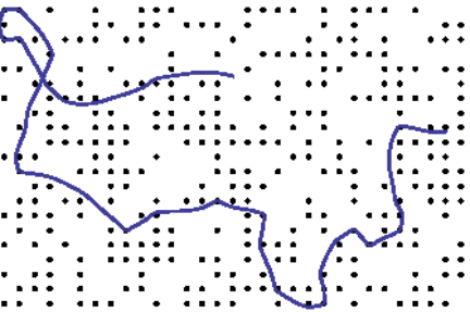
Refer to caption — Figure 4: Motion in the configuration space of a random coulombic potential

We restrict ourselves to dimension $d=2$ . Here for $j\in J$ the single site potentials

\tilde{W}_{j}\in C^{\eta}({\mathbb{R}}^{2}\setminus\{s_{j}\},{\mathbb{R}})

(with $\eta\in{\mathbb{N}}\cup\{\infty\},\eta\geq 2$ ) diverge at the position $s_{j}\in{\cal D}$ in the fundamental domain ${\cal D}:=\{x_{1}\ell_{1}+x_{2}\ell_{2}\mid 0\leq x_{i}<1\}$ of the lattice ${\mathcal{L}}=\mathrm{span}_{\mathbb{Z}}(\ell_{1},\ell_{2})$ .

Our assumptions are:

1.

The decay at infinity is short range, that is for $\alpha\in{\mathbb{N}}_{0}^{2},\ \lvert\alpha\rvert\leq\eta$

$\partial^{\alpha}\tilde{W}_{j}(q)={\cal O}(\lVert q\rVert^{-2-\varepsilon})\qquad(\lVert q\rVert\rightarrow\infty)\text{.}$

The local singularity at $s_{j}\in{\mathbb{R}}^{2}\cong{\mathbb{C}}$ is controlled by

f_{j}\colon{\mathbb{C}}^{*}:={\mathbb{C}}\setminus\{0\}\to{\mathbb{R}}\quad\text{,}\quad f_{j}(z):=\lvert z\rvert^{2}\tilde{W}_{j}(z^{2}+s_{j})

and we assume that for all multi–indices $\alpha\in{\mathbb{N}}_{0}^{2}$ , $\lvert\alpha\rvert\leq\eta$ , $\partial^{\alpha}f_{j}$ can be continuously extended to zero, with $f_{j}(0)<0$ . We allow for an additional single site potential $\tilde{W}_{0}=0$ .

Example 9.1.

The Yukawa Potential with parameters $c_{j},\mu_{j}>0$ is defined via

\tilde{W}_{j}(q)=-c_{j}\frac{\exp(-\mu_{j}\lVert q-s_{j}\rVert)}{\lVert q-s_{j}\rVert}\text{.}

Example 9.2.

Finite range potentials are given by

\tilde{W}_{j}(q):=-\frac{g_{j}(\lVert q-s_{j}\rVert)}{\lVert q-s_{j}\rVert}\text{,}

with $g_{j}\in C_{c}^{\eta}({\mathbb{R}},{\mathbb{R}}),\ g_{j}(0)>0$ .

The random potential is determined by the probability space $(\Omega,{\cal B}(\Omega),\beta)$ with $\Omega={\mathcal{L}}^{J}$ . The probability measure $\beta$ is assumed to be $\vartheta$ –invariant, see equation (2.2), and to give probability $\beta\{\omega_{0}\}=0$ to the configuration $\omega_{0}\in\Omega$ with $\omega_{0}(\ell)=0$ , $\ell\in{\mathcal{L}}$ . No ${\mathcal{L}}$ –ergodicity of $\beta$ is assumed here.

For what follows we fix $\omega\in\Omega$ . The punctured configuration space $\tilde{M}_{\omega}:={\mathbb{C}}\setminus{\cal S}_{\omega}$ now depends on the singularity set ${\cal S}_{\omega}:=\{s_{\omega(\ell)}+\ell\mid\ell\in{\mathcal{L}},\omega(\ell)\neq 0\}$ . The former supports the random potential

\tilde{V}_{\omega}\colon\tilde{M}_{\omega}\to{\mathbb{R}}\quad\text{,}\quad\tilde{V}_{\omega}(q):=\sum_{\ell\in{\mathcal{L}}}\tilde{W}_{\omega(\ell)}(q-\ell)\text{.}

Assumption 1. guarantees the convergence of $\tilde{V}_{\omega}$ and its derivatives, and Assumption 2. implies that the Coulombic singularities are attractive and

\tilde{V}_{\omega,\max}:=\sup\tilde{V}_{\omega}(\tilde{M}_{\omega})<\infty\text{.}

The Hamiltonian flow $\tilde{\Phi}_{\omega}\colon\tilde{U}_{\omega}\to\tilde{P}_{\omega}$ on $\tilde{P}_{\omega}:=T^{*}\tilde{M}_{\omega}={\mathbb{R}}^{2}\times\tilde{M}_{\omega}$ , generated by the Hamiltonian function $\tilde{H}_{\omega}\colon\tilde{P}\to{\mathbb{R}}$ , $(p,q)=\frac{1}{2}\lVert p\rVert^{2}+\tilde{V}_{\omega}(q)$ , is now, due to the Coulombic singularities, incomplete and only defined on a maximal open subset $\tilde{U}_{\omega}\subseteq{\mathbb{R}}\times\tilde{P}_{\omega}$ .

It is known that the flow can be continuously regularised by reflecting collision orbits at their singularity. This is possible, see Prop. 2.3 of [KK92] or Thm. 11.23 of [Kna11], by smoothly extending the incomplete Hamiltonian system

\big(\tilde{P}_{\omega},dq\wedge dp,\tilde{H}_{\omega}\big)\quad\text{ to a Hamiltonian system }\quad\big(P_{\omega},\sigma_{\omega},H_{\omega}\big)\text{,}

with $H_{\omega}\colon P_{\omega}\to{\mathbb{R}}$ generating a complete smooth Hamiltonian flow on the symplectic manifold $(P_{\omega},\sigma_{\omega})$ . In fact, similarly to the construction in Section 2, these data extend continuously to a triple $(P,\sigma,H)$ , with extended phase space $P:=\bigcup_{\omega\in\Omega}\ \{\omega\}\times P_{\omega}$ .

For $d=2$ and energies $E>V_{\max}$ regularization can also be performed, as in [Kna87, KK92], with the help of the twofold covering

\pi_{\omega}\colon\mathbf{M}_{\omega}:=\big\{(q,Q)\in{\mathbb{C}}^{2}\mid f_{\omega}(q)=Q^{2}\big\}\;\longrightarrow\;{\mathbb{C}}

(9.1)

with branch points in the singularity set ${\cal S}_{\omega}$ , where $f_{\omega}\colon{\mathbb{C}}\to{\mathbb{C}}$ is an entire function with simple zeroes in and only in ${\cal S}_{\omega}$ : $f_{\omega}^{-1}\{0\}={\cal S}_{\omega}$ . By a Weierstrass product construction we can choose $(\omega,q)\mapsto f_{\omega}(q)$ as a continuous function. The lift $\mathbf{\tilde{g}}_{\omega,E}:=(\pi_{\omega})^{*}\tilde{g}_{\omega,E}$ of the Jacobi-Maupertius metric

\tilde{g}_{\omega,E}(q):=\bigl(1-E^{-1}\tilde{V}_{\omega}(q)\bigr)g_{\mathrm{Euclid}}(q)\qquad(q\in{\hat{M}}_{\omega})

can be continued to all of $\mathbf{M}_{\omega}$ by taking limits:

\mathbf{g}_{\omega,E}(q,0):=\lim\limits_{\mathbf{M}_{\omega}\ni(q^{\prime},Q)\to(q,0)}\mathbf{\hat{g}}_{\omega,E}(q^{\prime},Q)\qquad(\pi_{\omega}(q)\in{\cal S}_{\omega})\text{,}

see [Kna87, KK92]. This gives a smooth and complete riemannian metric on $\mathbf{M}_{\omega}$ , and its geodesics are, up to a reparametrisation of time and modulo $\pi_{\omega}$ , trajectories of the Hamiltonian flow.

This geometric regularisation allows to take full advantage of riemannian geometry. For two-dimensional compact riemannian manifolds of negative curvature ergodicity of the geodesic flow was established by [Hop41]. The gaussian curvature of $({\hat{M}}_{\omega},\hat{g}_{\omega,E})$ at $q\in{\hat{M}}_{\omega}$ is given by

\begin{split}\tilde{K}_{\omega,E}(q)&=\frac{\bigl(E-\tilde{V}_{\omega}(q)\bigr)\Delta\tilde{V}_{\omega}(q)+\bigl(\nabla\tilde{V}_{\omega}(q)\bigr)^{2}}{2\bigl(E-\tilde{V}_{\omega}(q)\bigr)^{3}}\\ &=\frac{\bigl(1-E^{-1}\tilde{V}_{\omega}(q)\bigr)E^{-1}\Delta\tilde{V}_{\omega}(q)+\bigl(E^{-1}\nabla\tilde{V}_{\omega}(q)\bigr)^{2}}{2E\cdot\bigl(1-E^{-1}\tilde{V}_{\omega}(q)\bigr)^{3}}\text{.}\end{split}

(9.2)

Since $\pi_{\omega}^{-1}(\tilde{M}_{\omega})$ is a local isometry, the curvature of all non–branch points of $\mathbf{M}_{\omega}$ is determined by Equation 9.2. In Example 9.1 it turns out that for high enough energy $E>E_{\text{th}}>\tilde{V}_{\omega,\max}$ the curvature is non–positive. This motivates the following definition.

Definition 9.3.

The pair $(\tilde{V}_{\omega},E)$ is of non–positive (strictly negative) curvature, if $(\mathbf{M}_{\omega},\mathbf{g}_{\omega,E})$ has non–positive (strictly negative) curvature.

A direct consequence of equation (9.2) is, that, given a pair $(\tilde{V}_{\omega},E)$ of non–positive curvature, all $(\tilde{V}_{\omega},E^{\prime})$ with $E^{\prime}\geq E$ are of non–positive curvature, too. As $E\nearrow\infty$ the curvature concentrates in the singularities. In Example 9.2 non–positive curvature can be achieved for all energies above a threshold with suitable choices for $g_{j}$ , e.g.

g_{j}(r):=\begin{cases}-c_{j}\cos^{\eta+1}(\lambda_{j}r)&r<\frac{\pi}{2\lambda}\\ 0&r\geq\frac{\pi}{2\lambda}\end{cases}

with $c_{j},\lambda_{j}>0$ , see [Kna87]. From now on we will assume non–positive curvature. This assumption and the following lemma explain why we allow only $W_{0}=0$ as smooth single site potential.

Lemma 9.4.

If a single site potential $\tilde{W}\colon{\mathbb{C}}\to{\mathbb{R}}$ without singularity and an energy $E$ are of nonpositive curvature, then $\tilde{W}=\tilde{W}_{0}\equiv 0$ .

Proof:

From (2.1) it follows that the curvature of one single site potential is integrable. By the theorem of Gauss–Bonnet the integral of the curvature over ${\mathbb{C}}$ vanishes. Since the curvature is nonpositive, it has to vanish, too, and so does the single site potential. $\Box$

Our goal is

Theorem 9.5.

If $\,(\tilde{V}_{\omega},E)$ is of non–positive curvature, then the geodesic flow $\Phi_{\omega}\colon{\mathbb{R}}\times T_{1}\mathbf{M}_{\omega}\to T_{1}\mathbf{M}_{\omega}$ is topologically transitive $\beta$ –almost surely.

The strategy will be as follows. In Proposition 9.8 we show that the periodic orbits of $\Phi_{\omega}$ are dense in $T_{1}\mathbf{M}_{\omega}$ . Note, that the same is true for Anosov diffeomorphisms on compact manifolds, cf. [Bow75, 3.8]. Then, in the proof of Theorem 9.5 from page Proof on, in order to connect two open subsets of $T_{1}\mathbf{M}_{\omega}$ , we will connect two periodic orbits with an intertwining orbit.

We start with a useful lemma, which singles out the set of full measure on which we establish topological transitivity. We denote the Euclidean cone intersected with the lattice ${\mathcal{L}}$

\vartriangle_{q}^{(\varphi)}\!(x):=\{\ell\in{\mathcal{L}}\mid\sphericalangle(x,\ell-q)<\varphi\}\text{,}

$q\in{\mathbb{C}}$ , $\varphi\in[0,\pi]$ , $x\in T_{1,q}{\mathbb{C}}=S^{1}$ .

Lemma 9.6.

The $\vartheta$ –invariance of $\beta$ and $\beta\{\omega_{0}\}=0$ imply that there are $\beta$ -almost surely no Euclidean cones without nonvanishing single site potential. More precisely:

\beta\bigl\{\omega\in\Omega\bigm|\exists(q,\varphi,x)\in{\mathbb{R}}^{2}\times(0,\pi]\times S^{1}\colon\omega(\vartriangle_{q}^{(\varphi)}\!(x))=\{0\}\bigr\}=0\text{.}

Proof:

We study the sets

A_{q,\varphi,x}:=\bigl\{\omega\in\Omega\bigm|\omega\bigl(\vartriangle_{q}^{(\varphi)}\!(x)\bigr)=\{0\}\bigr\}\text{,}

$(q,\varphi,x)\in{\mathbb{R}}^{2}\times(0,\pi]\times S^{1}$ , first. For $(q,\varphi,\ell)\in{\mathbb{R}}^{2}\times(0,\pi]\times{\mathcal{L}}$ we have

\beta\bigl(A_{q,\varphi,\frac{\ell}{\lVert\ell\rVert}}\bigr)=\lim_{n\to\infty}\beta\bigl(A_{q-n\ell,\varphi,\frac{\ell}{\lVert\ell\rVert}}\bigr)=\beta\Bigl(\bigcap\nolimits_{n\in{\mathbb{N}}}A_{q-n\ell,\varphi,\frac{\ell}{\lVert\ell\rVert}}\Bigr)=\beta\{\omega_{0}\}=0\text{.}

Note now that the set in question can be written as the denumerable union

\bigcup\nolimits_{(q,\varphi,\ell)\in{\mathbb{Q}}^{2}\times{\mathbb{Q}}_{+}\times{\mathcal{L}}}A_{q,\varphi,\frac{\ell}{\lVert\ell\rVert}}\text{.}

$\Box$

We denote the tangent bundle of $\mathbf{M}_{\omega}$ with $\tau_{\mathbf{M}_{\omega}}\colon T\mathbf{M}_{\omega}\to\mathbf{M}_{\omega}$ and the natural length metric on $(\mathbf{M}_{\omega},\mathbf{g}_{\omega,E})$ with $d_{\mathbf{M}_{\omega}}$ .

Lemma 9.7.

For $\beta$ –almost all $\omega\in\Omega$ the following holds. Given a point $q\in\mathbf{M}_{\omega}$ and a nonempty open subset $U\subseteq T_{1,q}\mathbf{M}_{\omega}:=T_{1}\mathbf{M}_{\omega}\cap T_{q}\mathbf{M}_{\omega}$ of the sphere bundle, there exists an initial direction $v\in U$ such that the corresponding geodesic hits a branch point at $t>0$ , i.e.

\exp_{\mathbf{M}_{\omega}}(tv)\in\pi_{\omega}^{-1}({\cal S}_{\omega})\text{.}

Proof:

W.l.o.g. we assume $U\neq T_{1,q}\mathbf{M}_{\omega}$ . For every $\omega\in\Omega$ such that there is an open subset $U\subseteq T_{1,q}\mathbf{M}_{\omega}$ with no branch points in

\blacktriangle:=\exp_{\mathbf{M}_{\omega}}({\mathbb{R}}_{+}U)\;\subseteq\;\mathbf{M}_{\omega}

we will establish the existence of a Euclidean cone $\vartriangle\subseteq{\mathcal{L}}$ with $\omega(\vartriangle)=\{0\}$ . Then Lemma 9.6 applies and gives the desired result.

Fix $v\in U$ . Since the curvature of $(\mathbf{M}_{\omega},\mathbf{g}_{\omega,E})$ is nonpositive, we find a constant $\rho_{0}>0$ such that

d_{\mathbf{M}_{\omega}}\bigl(\exp_{\mathbf{M}_{\omega}}(tv),\,\mathbf{M}_{\omega}\setminus\blacktriangle\bigr)\;\geq\;2\rho_{0}t

(9.3)

for all $t\geq 0$ , see [BBI01]. Note that, due to the absence of branch points in $\blacktriangle$ , $\pi_{\omega}|_{\blacktriangle}$ is a homeomorphism onto its image, and since the conformal factor is bounded by $h:=1-E^{-1}\tilde{V}_{\omega,\max}$ , we know for all $q,q^{\prime}\in\mathbf{M}_{\omega}$

d_{\mathbf{M}_{\omega}}(q,q^{\prime})\;\leq\;h\cdot\lvert\pi_{\omega}(q)-\pi_{\omega}(q^{\prime})\rvert\text{.}

This implies

\blacktriangle^{\prime}\;:=\;\bigcup_{t\geq 0}B_{h^{-1}\rho_{0}t}\bigl(\pi_{\omega}\circ\exp_{\mathbf{M}_{\omega}}(tv)\bigr)\;\subseteq\;\pi_{\omega}(\blacktriangle)\;\subseteq\;{\mathbb{C}}\text{,}

and in $\blacktriangle^{\prime}$ we search our Euclidean cone $\vartriangle$ . All we have to show to this end is that the “axis” of $\blacktriangle^{\prime}$

{\mathbb{R}}_{+}\ni t\;\longmapsto\;\bigl(q_{\omega}(t),p_{\omega}(t)\bigr):=T\pi_{\omega}\circ\Phi_{\omega}(t,v)

converges to a definite direction: $\lim_{t_{0}\to\infty}\sup_{t\geq t_{0}}\lvert p_{\omega}(t+t_{0},v)-p_{\omega}(t_{0},v)\rvert=0$ . But this is clear from Assumption 1, i.e. that all single site potentials are short range, and equation (9.3), which together imply that the curvature along the axis vanishes. $\Box$

With this tools at hand it is easy to prove

Proposition 9.8.

The set of periodic orbits of $\Phi_{\omega}\colon{\mathbb{R}}\times T_{1}\mathbf{M}_{\omega}\to T_{1}\mathbf{M}_{\omega}$ is dense in $T_{1}\mathbf{M}_{\omega}$ for $\beta$ –almost every $\omega\in\Omega$ .

Proof:

To any nonempty open set $U\subseteq T_{1}\mathbf{M}_{\omega}$ we construct a periodic orbit whose trajectory intersects $U$ . Lemma 9.7 guarantees that we hit a branch point at some time $t>0$ . We choose a branch point

x\;\in\;\exp_{\mathbf{M}_{\omega}}(tU)\cap\pi_{\omega}^{-1}({\cal S}_{\omega})\;\subseteq\;\mathbf{M}_{\omega}\text{.}

Now $\Phi_{\omega}$ is continuous, which shows that

U^{\prime}:=-\Phi_{\omega}(t_{1},U)\cap T_{1,x}\mathbf{M}_{\omega}

is open in $T_{1,x}\mathbf{M}_{\omega}$ . Again by Lemma 9.7 we find $v\in U^{\prime}$ and $t^{\prime}>0$ such that $\Phi_{\omega}(t^{\prime},v)$ hits again a branch point. By construction the trajectory of $v$ intersects $U$ and is periodic. $\Box$

To gain more overview we introduce the universal covering $\mathbf{\pi}_{\omega}^{*}\colon\mathbf{M}_{\omega}^{*}\to\mathbf{M}_{\omega}$ of $\mathbf{M}_{\omega}$ and equipp it with the riemannian metric $\mathbf{g}_{\omega,E}^{*}:=(\mathbf{\pi}_{\omega}^{*})^{*}\mathbf{g}_{\omega,E}$ . This makes $\mathbf{M}_{\omega}^{*}$ a Hadamard manifold. We denote the natural length metric with $d_{\mathbf{M}_{\omega}^{*}}$ . The fact that there is a certain amount of negative curvature in $\mathbf{M}_{\omega}^{*}$ is expressed in the following.

Proposition 9.9.

For $\beta$ –almost all $\omega\in\Omega$ the riemannian surface $(\mathbf{M}_{\omega}^{*},\mathbf{g}_{\omega}^{*})$ is a visibility manifold, i.e. for all $p\in\mathbf{M}_{\omega}^{*}$ and $\varepsilon>0$ there exists $r=r(p,\varepsilon)>0$ such that all geodesic segments $\sigma\colon[a,b]\to\mathbf{M}_{\omega}^{*}$ with distance at least $r$ from $p$ are seen from $p$ under an angle less then $\varepsilon$ (cf. [EO73]):

\forall p\in\mathbf{M}_{\omega}^{*},\varepsilon>0\exists r>0\colon\quad d_{\mathbf{M}_{\omega}^{*}}(p,\sigma[a,b])\geq r\quad\implies\quad\sphericalangle_{p}\bigl(\sigma(a),\sigma(b)\bigr)<\varepsilon\text{.}

Proof:

We need to show that the set of all $\omega\in\Omega$ which allow a positive $\varepsilon$ such that we find for all $r>0$ a geodesic segment $\sigma_{r}\colon[a_{r},b_{r}]\to\mathbf{M}_{\omega}^{*}$ with

d_{\mathbf{M}_{\omega}^{*}}(p,\sigma_{r})>r

and 2.

\sphericalangle_{p}\bigl(\sigma_{r}(a_{r}),\sigma_{r}(b_{r})\bigr)\geq\varepsilon

is of $\beta$ –measure $0$ . To do this, we find a cone without singularities and invoke Lemma 9.7.

By compactness of $T_{1,p}\mathbf{M}_{\omega}^{*}$ we get $x,y\in T_{1,p}\mathbf{M}_{\omega}^{*}$ with $\sphericalangle_{p}(x,y)>\varepsilon$ and

d_{\mathbf{M}_{\omega}^{*}}(p,\gamma_{t})\xrightarrow{t\to\infty}\infty\text{,}

where $\gamma_{t}\colon[a_{t},b_{t}]\to\mathbf{M}_{\omega}^{*}$ is the unique geodesic segment connecting $\gamma_{t}(a_{t})=\exp_{\mathbf{M}_{\omega}^{*}}(tx)$ and $\gamma_{t}(b_{t})=\exp_{\mathbf{M}_{\omega}^{*}}(ty)$ .
The theorem of Gauss–Bonnet implies that the curvature integrated over the cone

\blacktriangle:=\bigcup_{t>0}\gamma_{t}[a_{t},b_{t}]

between $x$ and $y$ is bounded by $-\pi$ from below. This means that $\blacktriangle$ cannot cover two singularities, since then $\blacktriangle$ , beeing geodesically convex, would cover the periodic orbit connecting these two, and this would contradict Gauss–Bonnet. Thereby $\blacktriangle$ contains a cone without singularity and Lemma 9.7 applies. $\Box$

Remark 9.10.

Two geodesic rays $\gamma,\gamma^{\prime}\colon{\mathbb{R}}_{+}\to\mathbf{M}_{\omega}^{*}$ are called asymptotic, if their distance is bounded. Being asymptotic is an equivalence relation, and the set of equivalence classes (equipped with a suitable topology, see [EO73]) is the ideal boundary $\partial\mathbf{M}_{\omega}^{*}\equiv\mathbf{M}_{\omega}^{*}(\infty)$ of $\mathbf{M}_{\omega}^{*}$ . A point $\gamma(\infty):=[\gamma]\in\mathbf{M}_{\omega}^{*}(\infty)$ is a zero point, if for all $\gamma^{\prime}\in\gamma(\infty)$ the distance between $\gamma$ and $\gamma^{\prime}$ vanishes. [EO73] explains that a visibility manifold satisfies Axiom 1, i.e. any two distinct boundary points can be connected with a (not necessarily unique) geodesic.

Lemma 9.11.

For all $\omega\in\Omega$ holds the following. Every lift of a periodic geodesic in $\mathbf{M}_{\omega}$ to $\mathbf{M}_{\omega}^{*}$ connects two zero points of $\mathbf{M}_{\omega}^{*}(\infty)$ .

Proof:

Given a periodic geodesic $\gamma\colon S^{1}\to\mathbf{M}_{\omega}$ , its lift $\gamma^{*}\colon{\mathbb{R}}\to\mathbf{M}_{\omega}^{*}$ , and another geodesic $\gamma^{\prime}\colon{\mathbb{R}}\to\mathbf{M}_{\omega}^{*}$ with $\gamma^{*}(\infty)=\gamma^{\prime}(\infty)$ , we integrate curvature over the area bounded by $\gamma^{*}({\mathbb{R}}_{+})$ , $\gamma^{\prime}({\mathbb{R}}_{+})$ and the geodesic segment connecting $\gamma^{*}(0)$ and $\gamma^{\prime}(0)$ . Gauss–Bonnet assures us, that this quantity is bounded, and this is only possible if $\gamma^{*}$ and $\gamma^{\prime}$ have distance $0$ . Otherwise, since $\gamma^{*}$ covers a periodic orbit, the curvature integral is unbounded. $\Box$

Proof (of Theorem 9.5):

Proposition 9.8 tells us that for almost all $\omega\in\Omega$ periodic orbits of $\Phi_{\omega}$ are dense in $T_{1}\mathbf{M}_{\omega}$ . Therefore for any two open and nonempty sets $U,V\subseteq T_{1}\mathbf{M}_{\omega}$ we find two periodic geodesics $\gamma_{U},\gamma_{V}\colon{\mathbb{R}}\to\mathbf{M}_{\omega}$ which intersect $U$ and $V$ , respectively, i.e. $\dot{\gamma}_{U}({\mathbb{R}})\cap U\neq\emptyset$ and $\dot{\gamma}_{U}({\mathbb{R}})\cap V\neq\emptyset$ .

There are lifts $\gamma_{U}^{*},\gamma_{V}^{*}\colon{\mathbb{R}}\to\mathbf{M}_{\omega}^{*}$ of $\gamma_{U}$ and $\gamma_{V}$ to the universal covering $\mathbf{\pi}_{\omega}^{*}\colon\mathbf{M}_{\omega}^{*}\to M_{\omega}$ of $\mathbf{M}_{\omega}$ . By Propositions 9.9 and 9.10 the endpoints $\gamma_{U}^{*}(-\infty)$ and $\gamma_{V}^{*}(\infty)$ can be joined with a geodesic $\gamma^{*}\colon{\mathbb{R}}\to\mathbf{M}_{\omega}^{*}$ , i.e. $\gamma^{*}(-\infty)=\gamma_{U}^{*}(-\infty)$ and $\gamma^{*}(\infty)=\gamma_{V}^{*}(\infty)$ . Lemma 9.11 makes sure that the distance between $\gamma^{*}(t)$ and $\gamma_{U}^{*}\bigl((0,\infty)\bigr)$ respectively $\gamma_{V}^{*}\bigl((-\infty,0)\bigr)$ vanishes, as $t\to\pm\infty$ , respectively:

\lim_{t\to\infty}d_{\mathbf{M}_{\omega}^{*}}\bigl(\gamma^{*}(t),\gamma_{U}^{*}\bigl((0,\infty)\bigr)\bigr)=\lim_{t\to-\infty}d_{\mathbf{M}_{\omega}^{*}}\bigl(\gamma^{*}(t),\gamma_{V}^{*}\bigl((-\infty,0)\bigr)\bigr)=0\text{.}

This implies that $T\mathbf{\pi}_{\omega}^{*}\circ\dot{\gamma}^{*}({\mathbb{R}})$ intersects $U$ and $V$ . $\Box$

10 Ergodicity of the finite factor

Similar to the lattice and the poissonian case, the Coulombic system does have a finite factor. Assuming $(\vartheta,\beta)$ to be ergodic again and the single site potentials to be $\eta\geq 3$ times continuously differentiable, we show ergodicity of this factor. This is analogous to a result in [Len03] in the setting of billiards. Thanks to the smoothness of our system, our proof can rely directly on [Hop41] without the need for technical generalisations to cope with singularities like e.g. in [LW95].

The following construction of the finite factor is carried out in detail in [Sch04, Sch10]. As above the geodesic motion on the energy surface is regularised with the twofold covering (9.1). There is one nontrivial deck transformation

\mathbf{G}_{\omega}\colon\mathbf{M}_{\omega}\to M_{\omega}\text{,}\quad G(q,Q):=(q,-Q)\text{.}

For each $\omega\in\Omega$ and every $\ell\in{\mathcal{L}}$ there exists an isometry

\mathbf{\phi}_{\omega,\ell}\colon\mathbf{M}_{\omega}\to\mathbf{M}_{\vartheta_{\ell}\omega}

that shifts $q$ to $q-\ell$ :

\pi_{\vartheta_{\ell}\omega}\circ\mathbf{\phi}_{\omega,\ell}(q,Q)\;=\;q-\ell\qquad\bigl((q,Q)\in\mathbf{M}_{\omega}\bigr)\text{.}

The deck transformation gives another such map $\mathbf{\phi}_{\omega,\ell}\circ\mathbf{G}_{\omega}=\mathbf{G}_{\vartheta_{\ell}\omega}\circ\mathbf{\phi}_{\omega,\ell}$ . Before we can bundle the maps $\bigl((\mathbf{\phi}_{\omega,\ell})_{\omega\in\Omega}\bigr)_{\ell\in{\mathcal{L}}}$ into a group action of ${\mathcal{L}}$ on $\mathbf{M}:=\bigcup_{\omega\in\Omega}\{\omega\}\times\mathbf{M}_{\omega}$ , we have to divide through the group of deck transformations.

But $\pi_{\omega}$ is a branched covering, so to keep the differentiable structure we first follow [Kna87, KK92] and restrict the geodesic flow to the energy surface

\mathbf{\Sigma}_{\omega,E}:=\big\{(x,v)\in T{\mathbb{C}}^{2}\mid\mathbf{g}_{\omega,E}(v,v)=1\big\}\text{.}

We divide $\mathbf{\Sigma}_{\omega,E}$ by the group ${\mathbb{Z}}_{2}\cong\big\{\mathrm{Id}_{\mathbf{\Sigma}_{\omega,E}},D\mathbf{G}_{\omega}{\upharpoonright}_{\mathbf{\Sigma}_{\omega,E}}\big\}$ and get the smooth manifold

\Sigma_{\omega,E}:=\mathbf{\Sigma}_{\omega,E}/{\mathbb{Z}}_{2}\text{.}

The disjoint union

\mathbf{\Sigma}_{E}:=\bigcup_{\omega\in\Omega}\{\omega\}\times\mathbf{\Sigma}_{\omega,E}

inherits its topology from the embedding into $\Omega\times T{\mathbb{C}}^{2}$ . The quotient

\Sigma_{E}:=\mathbf{\Sigma}_{E}/{\mathbb{Z}}_{2}=\bigcup_{\omega\in\Omega}\{\omega\}\times\Sigma_{\omega,E}

is the phase space for which we can construct the desired group action

\Theta^{E}\colon{\mathcal{L}}\times\Sigma_{E}\to\Sigma_{E}\text{,}\quad\Theta^{E}_{\ell}\bigl(\omega,[x]_{{\mathbb{Z}}_{2}}\bigr):=\bigl(\vartheta_{\ell}\omega,[D\mathbf{\phi}_{\omega,\ell}(x)]_{{\mathbb{Z}}_{2}}\bigr)\text{.}

This group action is continuous. Analogous to Section 2 the quotient

\pi_{\mathcal{L}}\colon\Sigma_{E}\to\hat{\Sigma}_{E}:=\Sigma_{E}/{\mathcal{L}}

is compact and metrizable, inherits the geodesic flow

\hat{\Phi}_{E}\colon{\mathbb{R}}\times\hat{\Sigma}_{E}\to\hat{\Sigma}_{E}

and carries the finite and $\hat{\Phi}_{E}$ –invariant Liouville measure $\hat{\mu}_{E}$ , see [Sch10]. An overview over the different phase spaces including the embedding into $\Omega\times T{\mathbb{C}}^{2}$ and the unit tangent bundle $\mathbf{\Sigma}_{\omega,E}^{*}$ of the universal cover $\mathbf{\pi}_{\omega}^{*}\colon\mathbf{M}_{\omega}^{*}\to\mathbf{M}_{\omega}$ is given in Figure 5.

\begin{CD}\mathbf{\Sigma}_{\omega,E}^{*}@>{\mathbf{\Pi}_{\omega}^{*}}>{}>\mathbf{\Sigma}_{\omega,E}@>{}>{}>\mathbf{\Sigma}_{E}@>{}>{}>\Omega\times T{\mathbb{C}}^{2}\\ &&@V{}V{\pi_{\omega,{\mathbb{Z}}_{2}}}V@V{}V{\pi_{{\mathbb{Z}}_{2}}}V\\ &&\Sigma_{\omega,E}@>{\iota_{\omega,E}}>{}>\Sigma_{E}@>{\pi_{{\mathcal{L}}}}>{}>\hat{\Sigma}_{E}\phantom{\times T{\mathbb{C}}^{2}}\end{CD}

Figure 5: Overview over the relations between the different phase spaces

Theorem 10.1.

Let the shift action $\vartheta\colon{\mathcal{L}}\times\Omega\to\Omega$ be ergodic with respect to $\beta$ , the potential $\tilde{V}_{\omega}$ three times continuous differentiable and $(\tilde{V}_{\omega},E)$ of strictly negative curvature for $\beta$ -almost all $\omega\in\Omega$ .
Then the flow $\hat{\Phi}_{E}$ is ergodic with respect to $\hat{\mu}_{E}$ .

Proof:

In [Hop41] the ergodicity of a recurrent and hyperbolic geodesic flow on a $2$ -dimensional riemannian surface is proven. We use that work here.

We need to show that for every continuous function $\hat{f}\colon\hat{\Sigma}_{E}\to{\mathbb{R}}$ the limits

\bar{f}^{\pm}:=\lim_{T\to\pm\infty}\frac{1}{T}\int_{0}^{T}\hat{f}\circ\hat{\Phi}_{E}(t,\cdot)\,dt

(10.1)

exist and are almost everywhere constant. The existence a.e. of $\bar{f}^{\pm}$ is guaranteed by Birkhoff’s ergodic theorem, and so is $\bar{f}^{+}=\bar{f}^{-}=:\bar{f}$ $\hat{\mu}_{E}$ -a.e..

Via the quotients and embeddings, see Figure 5, we introduce

f_{\omega}^{*}\colon\mathbf{\Sigma}_{\omega,E}^{*}\to{\mathbb{R}}\text{,}\quad f_{\omega}^{*}:=\hat{f}\circ\pi_{\mathcal{L}}\circ\iota_{\omega,E}\circ\pi_{\omega,{\mathbb{Z}}_{2}}\circ\mathbf{\Pi}_{\omega}^{*}\quad(\omega\in\Omega)\text{.}

By Poincaré’s recurrence theorem the finite measure preserving dynamical system $(\hat{\Sigma}_{E},\hat{\Phi}_{E},\hat{\mu}_{E})$ is recurrent, so that $\liminf_{t\to\infty}\lvert f_{\omega}^{*}\circ(\mathbf{\Phi}_{\omega,E}^{*})_{t}-f_{\omega}^{*}\rvert=0$ a.e., see e.g. [Aar97, p. 14–16]. Hyperbolicity is guaranteed by the curvature assumption. Using the a.e. constancy of $\bar{f}_{\omega}^{*}$ along stable and unstable manifolds like in [Hop41] we see, that for each $\omega\in\Omega$ the limit $\bar{f}_{\omega}^{*}$ is almost surely constant.

Finally we use the ergodicity of $(\vartheta,\beta)$ to conclude that $\bar{f}$ ist constant on $\hat{\Sigma}_{E}$ . By denoting this a.e.-value by $F(\omega)$ for $\beta$ -a.a. $\omega\in\Omega$ we define $\beta$ -a.e. a function $F\colon\Omega\to{\mathbb{R}}$ . Since the whole construction depends measurably on $\omega\in\Omega$ , $F$ itself is measurable. To see that $F$ is in fact $\vartheta$ –invariant, we introduce

f_{\Sigma_{E}}:=\bar{f}\circ\pi_{\mathcal{L}}\colon\Sigma_{E}\to{\mathbb{R}}\qquad(\omega\in\Omega)

(10.2)

and write for a.e. $\omega\in\Omega$ , a.e. $x\in\Sigma_{\vartheta_{\ell}\omega}$ and a.e. $y\in\Sigma_{\omega}$

\displaystyle F(\vartheta_{\ell}\omega)

\displaystyle=f_{\Sigma_{E}}\circ\iota_{\vartheta_{\ell}\omega}(x)=f_{\Sigma_{E}}\circ\Theta^{E}\circ\iota_{\omega}(y)=f_{\Sigma_{E}}\circ\iota_{\omega}(y)=F(\omega)\text{,}

using that $f_{\Sigma_{E}}$ by definition is $\Theta^{E}$ –invariant, see Equations 10.1 and 10.2. Therefore, by ergodicity of $(\vartheta,\beta)$ , $F$ is $\beta$ -a.s. constant, which then implies that $\bar{f}$ is constant modulo $\hat{\mu}_{E}$ . $\Box$

The above theorem relates to a geodesic flow on a (extended and compactified) unit tangent bundle. This construction has been made in order to make use of the well-known consequences of negative curvature on the dynamics.
Like in the case of smooth potentials treated in Section 6, we are finally interested in the (analog of) the Hamiltonian flow (6.1) generated by $\hat{H}$ (based on the Hamiltonian $H\colon P\to{\mathbb{R}}$ on the extended phase space $P$ of the first regularization in Section 9). As this flow is related to the geodesic flow of Theorem 10.1 by a continuous time change, we get:

Corollary 10.2.

Under the conditions of Theorem 10.1 the coulombic Hamiltonian flow (6.1) on the compactified energy surface $\hat{\Sigma}_{E}$ is ergodic w.r.t. Liouville measure ${\hat{\lambda}}_{E}$ .

Remark 10.3 (Markov Partition).

In a forthcoming article, one of us (CS) shows for all large energies, under some additional conditions, the existence of Markov partitions for the system, cf. [Sch10].

In [CLS10] Cristadoro, Lenci and Seri show recurrence for random Lorenz tubes. Their configuration spaces are contained in a connected union of translates of a fundamental polygon. We a have similar statement for the Coulomb case.

Again with $H\colon P\to{\mathbb{R}}$ from Section 9, for $\ell\in{\mathcal{L}}\setminus\{0\}$ we define the factors

\check{\Sigma}_{E}:=H^{-1}(E)/\mathrm{span}_{{\mathbb{Z}}}(\ell)\quad\text{and}\quad\check{\Sigma}_{E,\omega}:=H_{\omega}^{-1}(E)/\mathrm{span}_{{\mathbb{Z}}}(\ell)\text{,}

for $\ell$ –periodic $\omega\in\Omega$ . Again we assume $(V_{\omega},E)$ to be of strictly negative curvature $\beta$ –a.s.. As we divided by the free $\Theta$ –action of a subgroup of ${\mathcal{L}}$ , by the analog of (2.4) we obtain smooth flows on the non–compact three–manifolds $\check{\Sigma}_{E,\omega}$ .

We assume for simplicity that $\ell\in{\mathcal{L}}$ is primitive. Then ${\mathcal{L}}/\mathrm{span}_{{\mathbb{Z}}}(\ell)\cong{\mathbb{Z}}$ (and via the element $\ell^{\prime}$ of a positively oriented basis $(\ell,\ell^{\prime})$ of ${\mathcal{L}}$ , this isomorphism is unique). We may consider random potentials indexed by $\Omega_{\ell}:=J^{\mathbb{Z}}$ . ${\mathbb{Z}}$ –ergodic probability measures $\beta_{\ell}$ on $\Omega_{\ell}$ give rise to ${\mathcal{L}}$ –ergodic image measures $\beta$ on $\Omega$ , via the injection $\mathbf{i}\colon\Omega_{\ell}\to\Omega$ , ${\bf i}(\omega)_{a\ell+b\ell^{\prime}}=\omega_{b}$ . These are analogues of the measures considered in [CLS10]. For non–trivial $\beta_{\ell}$ the flow on $\check{\Sigma}_{E}$ is not ergodic w.r.t. the measure induced by $\check{\mu}_{E}$ via the projection $\check{\Sigma}_{E}\to\hat{\Sigma}_{E}$ .

Proposition 10.4 (Ergodicity and Recurrence of Coulomb Tubes).

Under
the conditions of Theorem 10.1

•

$\beta$ –a.s. the motion on $\check{\Sigma}_{E}$ is recurrent.
•

For ${\bf i}(\beta_{\ell})$ –almost all $\omega\in\Omega$ the motion on $\check{\Sigma}_{E,\omega}$ is recurrent and ergodic.

Proof:

By Corollary 10.2 the flow $\hat{\Phi}_{E}$ is ergodic w.r.t. ${\hat{\lambda}}_{E}$ . Thus by the analog of Proposition 6.5 for Coulomb potentials, for $\beta$ –a.e. $\omega$ the asymptotic velocity ${\overline{v}}(x)=0$ a.e. on $\Sigma_{E,\omega}$ , and thus on $\check{\Sigma}_{E}$ . If $\beta$ is of the form ${\bf i}(\beta_{\ell})$ , then for $\beta$ –a.e. $\omega$ the asymptotic velocity ${\overline{v}}(x)=0$ a.e. on $\check{\Sigma}_{E,\omega}$ .

We compare with Schmidt [Sch98] (and the references cited therein). In the case of an ergodic transformation $T$ on a standard probability space $(X,\mu)$ , a Borel map $f\colon X\rightarrow{\mathbb{R}}$ and the induced cocycle (orbit sum) $\hat{f}\colon{\mathbb{Z}}\times X\rightarrow{\mathbb{R}}$ , he defines $\sigma_{k}(A):=\mu(\{x\in X\mid\hat{f}(k,x)/k\in A\})\quad(k\in{\mathbb{N}})$ , for Borel sets $A\subseteq{\mathbb{R}}$ .

Under the assumption that vaguely $\lim_{k\rightarrow\infty}\sigma_{k}=\delta_{0}$ , he notes that $f$ is recurrent, meaning that $\liminf_{k\rightarrow\infty}\lvert\hat{f}(k,x)\rvert=0$ , $\mu$ –a.s..

Here we use a Poincaré map discretization $(X,\mu,T)$ of the flow $\hat{\Phi}_{E}$ on $\hat{\Sigma}_{E}$ (by Remark 10.3 such a discretization exists and is ergodic). For $f(x_{0})$ , with $x_{0}=[(\omega,p_{0},q_{0})]\in X$ , we use the difference $\left\langle q(T(x_{0}))-q_{0},\ell^{\perp}\right\rangle$ in position along the direction $\ell^{\perp}:=\left(\begin{smallmatrix}0&1\\ -1&0\end{smallmatrix}\right)\ell\in{\mathbb{R}}^{2}$ perpendicular to $\ell$ . $f$ is well-defined on $X$ .

The assumptions of [Sch98] apply and $f$ is recurrent. This means that for a.e. $x_{0}$ the motion in the Coulomb tube returns infinitely often to every neighbourhood of the circle in the configuration torus given by $\left\langle q_{0},\ell^{\perp}\right\rangle=0$ . Then one obtains, by Poincaré’s Recurrence Theorem for the induced map, recurrence in the usual sense.

Ergodicity of the flow on $\check{\Sigma}_{E,\omega}$ follows from local ergodicity, using Hopf’s argument [Hop39]. $\Box$

References

[Aar97] Jon Aaronson. An Introduction to Infinite Ergodic Theory, volume 50 of Mathematical Surveys and Monographs. American Mathematical Society, 1997.
[AK98] Joachim Asch and Andreas Knauf. Motion in Periodic Potentials. Nonlinearity, 11(1):175–200, Jan 1998.
[AM78] Ralph Abraham and Jerrold E. Marsden. Foundations of Mechanics. The Benjamin/Cummings Publishing company, Inc., 2nd edition, 1978.
[Arn78] Vladimir Igorevic̆ Arnol’d. Mathematical Methods of Classical Mechanics. Springer-Verlag, Berlin Heidelberg New York, 1978.
[BBI01] Dimitri Burago, Yuri Burago, and Sergei Ivanov. A Course in Metric Geometry, volume 33 of Graduate Studies in Mathematics. American Mathematical Society, 2001.
[Bow75] Rufus Bowen. Equilibrium states and the ergodic theory of Anosov diffeomorphisms. Springer-Verlag, 1975.
[BS81] L. A. Bunimovich and Ya. G. Sinai. Statistical properties of lorentz gas with periodic configuration of scatterers. Communications in Mathematical Physics, 78:479–497, 1981.
[CLS10] Giampaolo Cristadoro, Marco Lenci, and Marcello Seri. Recurrence for quenched random Lorentz tubes. Chaos, 20:023115, 2010.
[DL91] Victor Donnay and Carlangelo Liverani. Potentials on the two–torus for which the Hamiltonian flow is ergodic. Communications in Mathematical Physics, 135:267–302, 1991.
[EO73] P. Eberlein and B. O’Neill. Visibility Manifolds. Pacific Journal of Mathematics, 46:45–109, 1973.
[GHL48] Sylvestre Gallot, Dominique Hulin, and Jaques Lafontaine. Riemannian Geometry. Springer-Verlag, 1948.
[Hir76] Morris W. Hirsch. Differential Topology, volume 33 of Graduate Texts in Mathematics. Springer-Verlag, 1976.
[Hop39] Eberhard Hopf. Statistik der geodätischen Linien in Mannigfaltigkeiten negativer Krümmung. Ber. Verh. Sächs. Akad. Wiss. Leipzig, 91:261–304, 1939.
[Hop41] Eberhard Hopf. Statistik der Lösungen geodätischer Probleme vom unstabilen Typus II. Mathematische Annalen, 117:590–608, 1941.
[Kel98] Gerhard Keller. Equilibrium States in Ergodic Theory, volume 42 of London Mathematical Society Student Texts. Cambridge University Press, 1998.
[KK92] Markus Klein and Andreas Knauf. Classical Planar Scattering by Coulombic Potentials, volume 13 of Lecture Notes in Physics. Springer-Verlag, Berlin Heidelberg New York, 1992.
[KK08] Andreas Knauf and Markus Krapf. The non-trapping degree of scattering. Nonlinearity, 21:2023–2041, 2008.
[Kli95] Wilhelm P. A. Klingenberg. Riemannian Geometry, volume 1 of de Gruyter Studies in Mathematics. de Gruyter, 2nd edition, 1995.
[Kna87] Andreas Knauf. Ergodic and Topological Properties of Coulombic Periodic Potentials. Commun. Math. Phys., 110:89–112, 1987.
[Kna90] Andreas Knauf. Closed orbits and converse KAM theory. Nonlinearity, 3:961–973, 1990.
[Kna11] Andreas Knauf. Mathematische Physik: Klassische Mechanik. Master Class. Springer, 2011.
[Len03] Marco Lenci. Aperiodic Lorentz gas: recurrence and ergodicity. Ergodic Theory and Dynamical Systems, 23:869–883, 2003.
[LMW03] Hajo Leschke, Peter Müller, and Simone Warzel. A survey of rigorous results on random Schrödinger operators for amorphous solids. Markov Processes and Related Fields, 9:729–760, 2003.
[LW95] Carlangelo Liverani and Maciej P. Wojtkowski. Ergodicity in Hamiltonian systems. In Dynamics reported, volume 4 of Dynam. Report. Expositions Dynam. Systems (N.S.), pages 130–202. Springer, Berlin, 1995.
[Nat01] Frank Natterer. The Mathematics of Computerized Tomography. Classics in Applied Mathematics. Society for Industrial Mathematics, 2001.
[PF92] Leonid Andreevich Pastur and Alexander Figotin. Spectra of Random and Almost-Periodic Operators, volume 297 of Grundlehren der mathematischen Wissenschaften. Springer-Verlag, 1992.
[Pös82] Jürgen Pöschel. Integrability of Hamiltonian Systems on Cantor Sets. Commun. Pure Appl. Math., 35:653–695, 1982.
[PP94] Gabriel P. Paternain and Miguel Paternain. On Anosov Energy Levels of Convex Hamiltonian Systems. Mathematische Zeitschrift, 217(1):367–376, September 1994.
[RF11] Wojciech De Roeck and Jürg Fröhlich. Diffusion of a massive quantum particle coupled to a quasi-free thermal medium. Commun. Math. Phys., 303:613–707, 2011.
[Rue87] David Ruelle. A Mathematical Reformulation of Derrida’s REM and GREM. Commun. Math. Phys., 108:225–239, 1987.
[Sch98] Klaus Schmidt. On joint recurrence. C. R. Acad. Sci. Paris, 327:837–842, 1998.
[Sch04] Christoph Schumacher. Klassische Bewegung in zufälligen Potenzialen. Diplomarbeit, 2004.
[Sch10] Christoph Schumacher. Klassische Bewegung in zufälligen Potenzialen mit Coulomb-Singularitäten. PhD Thesis, 2010.
[SKM87] Dietrich Stoyan, W. S. Kendall, and Joseph Mecke. Stochastic Geometry and Its Applications. Applied Probability and Statistics. John Wiley & Sons, 1987.
[Ves08] Ivan Veselić. Existence and regularity properties of the integrated density of states of random Schrödinger operators, volume 1917 of Lecture Notes in Mathematics. Springer-Verlag, Berlin Heidelberg New York, 2008.
[Wal82] Peter Walters. An Introduction to Ergodic Theory, volume 79 of Graduate Texts in Mathematics. Springer-Verlag, 1982.

Classical Motion in Random Potentials

Abstract

1 Introduction

2 The Lattice Case

Remark 2.1.

Remark 2.2 (Non–Existence of Asymptotic Velocity).

Proposition 2.3.

Proof:

Corollary 2.4.

Proof:

3 Distribution of Asymptotic Velocities

Proposition 3.1.

Proof:

Proposition 3.2.

Proof:

Definition 3.3.

Proposition 3.4.

Proof:

Proposition 3.5.

Remark 3.6.

Proof:

Example 3.7 (Random Potential With Non-Zero Asymptotic Velocity).

4 Poisson Potentials

Proposition 4.1.

Proof:

Remark 4.2 (Comparison With Quantum Mechanics).

Lemma 4.3.

Proof:

Proposition 4.4.

Proof:

Remarks 4.5.

5 Singular Values of the Hamiltonian

Proposition 5.1.

Proof:

Example 5.2 (Denseness of Singular Values).

Proposition 5.3.

Proof:

Remark 5.4 (Denseness of Singular Values, Poisson Case).

6 Notions of Ergodicity of Time Evolution

Proposition 6.1.

Proof:

Proposition 6.2.

Remark 6.3.

Proof:

Proposition 6.4.

Proof:

Proposition 6.5.

Proof:

7 No Ergodicity in the Poisson Case

Theorem 7.1.

Lemma 7.2.

Proof:

Proof (The Case I>0I>0):

Proof (The Case I<0I<0):

Proof (The Case I=0I=0):

8 No Hyperbolicity for Bounded Potentials

Example 8.1.

Theorem 8.2 (G. P. and M. Paternain).

Proof:

Remark 8.3 (The Non-Wandering Condition).

Theorem 8.4.

Proof:

9 Random Coulombic Potentials

Example 9.1.

Example 9.2.

Definition 9.3.

Lemma 9.4.

Proof:

Theorem 9.5.

Lemma 9.6.

Proof:

Lemma 9.7.

Proof:

Proposition 9.8.

Proof:

Proposition 9.9.

Proof:

Remark 9.10.

Lemma 9.11.

Proof:

Proof (The Case $I>0$ ):

Proof (The Case $I<0$ ):

Proof (The Case $I=0$ ):