Joint Spectral Radius and
Path-Complete Graph Lyapunov FunctionsThanks: A shorter and preliminary version of this work has been
presented in [4] as a conference paper.
Abstract
We introduce the framework of path-complete graph Lyapunov functions for approximation of the joint spectral radius. The approach is based on the analysis of the underlying switched system via inequalities imposed among multiple Lyapunov functions associated to a labeled directed graph. Inspired by concepts in automata theory and symbolic dynamics, we define a class of graphs called path-complete graphs, and show that any such graph gives rise to a method for proving stability of the switched system. This enables us to derive several asymptotically tight hierarchies of semidefinite programming relaxations that unify and generalize many existing techniques such as common quadratic, common sum of squares, path-dependent quadratic, and maximum/minimum-of-quadratics Lyapunov functions. We compare the quality of approximation obtained by certain classes of path-complete graphs including a family of dual graphs and all path-complete graphs with two nodes on an alphabet of two matrices. We derive approximation guarantees for several families of path-complete graphs, such as the De Bruijn graphs. This provides worst-case perfomance bounds for path-dependent quadratic Lyapunov functions and a constructive converse Lyapunov theorem for maximum/minimum-of-quadratics Lyapunov functions.
keywords
joint spectral radius, stability of switched systems, linear difference inclusions, finite automata, Lyapunov methods, semidefinite programming.1 Introduction
Given a finite set of square matrices , their joint spectral radius is defined as
| (1) |
where the quantity is independent of the norm used in (1). The joint spectral radius (JSR) is a natural generalization of the spectral radius of a single square matrix and it characterizes the maximal growth rate that can be obtained by taking products, of arbitrary length, of all possible permutations of . This concept was introduced by Rota and Strang [48] in the early 60s and has since been the subject of extensive research within the engineering and the mathematics communities alike. Aside from a wealth of fascinating mathematical questions that arise from the JSR, the notion emerges in many areas of application such as stability of switched linear dynamical systems, Leontief input-output model of the economy with uncertain data, computation of the capacity of codes, continuity of wavelet functions, convergence of consensus algorithms, trackability of graphs, and many others. See [33] and references therein for a recent survey of the theory and applications of the JSR.
Motivated by the abundance of applications, there has been much work on efficient computation of the joint spectral radius; see e.g. [21], [11], [10], [36], [43], [38], [25], [26], [24] and references therein. Unfortunately, the negative results in the literature certainly restrict the horizon of possibilities. In [12], Blondel and Tsitsiklis prove that even when the set consists of only two matrices, the question of testing whether is undecidable. They also show that unless P=NP, one cannot compute an approximation of that satisfies , in a number of steps polynomial in the bit size of and the bit size of [50]. It is easy to show that the spectral radius of any finite product of length raised to the power of gives a lower bound on [33]. However, for reasons that we explain next, our focus will be on computing upper bounds for .
There is an attractive connection between the joint spectral radius and the stability properties of an arbitrarily switched linear system; i.e., dynamical systems of the form
| (2) |
where is a map from the set of integers to the set of indices. It is well-known that if and only if system (2) is absolutely asymptotically stable (AAS), that is, (globally) asymptotically stable for all switching sequences. Moreover, it is known [39] that absolute asymptotic stability of (2) is equivalent to absolute asymptotic stability of the linear difference inclusion
| (3) |
where here denotes the convex hull of the set . Therefore, any method for obtaining upper bounds on the joint spectral radius provides sufficient conditions for stability of systems of type (2) or (3). Conversely, if we can prove absolute asymptotic stability of (2) or (3) for the set for some positive scalar , then we get an upper bound of on . (This follows from the scaling property of the JSR: .) One advantage of working with the notion of the joint spectral radius is that it gives a way of rigorously quantifying the performance guarantee of different techniques for stability analysis of systems (2) or (3).
Perhaps the most well-established technique for proving stability of switched systems is the use of a common (or simultaneous) Lyapunov function. The idea here is that if there is a continuous, positive, and homogeneous (Lyapunov) function that for some satisfies
| (4) |
(i.e., decreases no matter which matrix is applied), then the system in (2) (or in (3)) is AAS. Conversely, it is known that if the system is AAS, then there exists a convex common Lyapunov function (in fact a norm); see e.g. [33, p. 24]. However, this function is not in general finitely constructable. A popular approach has been to try to approximate this function by a class of functions that we can efficiently search for using convex optimization and in particular semidefinite programming. Semidefinite programs (SDPs) can be solved with arbitrary accuracy in polynomial time and lead to efficient computational methods for approximation of the JSR. As an example, if we take the Lyapunov function to be quadratic (i.e., ), then the search for such a Lyapunov function can be formulated as the following SDP:
| (5) |
The quality of approximation of common quadratic Lyapunov functions is a well-studied topic. In particular, it is known [11] that the estimate obtained by this method11 1 The estimate is the reciprocal of the largest that satisfies (5) and can be found by bisection. satisfies
| (6) |
where is the dimension of the matrices. This bound is a direct consequence of John’s ellipsoid theorem and is tight [7]. Morover, it is known that applying the common quadratic method to products of increasing length from the set gives an asymptotically exact method for the computation of the JSR [7], [9].
In [43], the use of sum of squares (SOS) polynomial Lyapunov functions of degree was proposed as a common Lyapunov function for the switched system in (2). The search for such a Lyapunov function can again be formulated as a semidefinite program. This method does considerably better than a common quadratic Lyapunov function in practice and its estimate satisfies the bound
| (7) |
where . Furthermore, as the degree goes to infinity, the estimate converges to the true value of [43].
The semidefinite programming based methods for approximation of the JSR have been recently generalized and put in the framework of conic programming [45]. We shall also remark that there are powerful techniques for approximation of the JSR that do not use semidefinite programming, such as approaches based on computation of a polytopic norm [24], [25], [26]. Research in the computation of the JSR continues to be an active area and each novel technique has the potential to enhance not only our ability to solve certain instances more efficiently, but also our understanding of the relations between the different approaches. An increasing number of the currently available methods for JSR approximation are being (or have been) implemented in the JSR Toolbox, a MATLAB based software package freely available for download [17]. Extensive numerical experiments comparing some of the different approaches have been carried out using this toolbox and recently reported in [14].
1.1 Contributions and organization
It is natural to ask whether one can develop better approximation schemes for the joint spectral radius by using multiple Lyapunov functions as opposed to requiring simultaneous contractibility of a single Lyapunov function with respect to all the matrices. More concretely, our goal is to understand in what ways we can write inequalities among, say, different Lyapunov functions that imply absolute asymptotic stability of (2) and can be checked via semidefinite programming.
The general idea of using several Lyapunov functions for analysis of switched systems is a very natural one and has already appeared in the literature (although to our knowledge not in the context of the approximation of the JSR); see e.g. [32], [13], [15], [36], [38], [35], [37], [30], [29], [20]. Perhaps one of the earliest references is the work on “piecewise quadratic Lyapunov functions” in [32]. However, this work is in the different framework of state dependent switching, where the dynamics switches depending on which region of the space the trajectory is traversing (as opposed to arbitrary switching). In this setting, there is a natural way of using several Lyapunov functions: assign one Lyapunov function per region and “glue them together”. Closer to our setting, there is a body of work in the literature that gives sufficient conditions for existence of piecewise Lyapunov functions of the type , , and , i.e., the pointwise maximum, the pointwise minimum, and the convex envelope of a set of quadratic functions [30], [29], [20], [31]. These works are mostly concerned with analysis of linear differential inclusions in continuous time, but they have obvious discrete time counterparts. The main drawback of these methods is that in their greatest generality, they involve solving bilinear matrix inequalities, which are non-convex and in general NP-hard. One therefore has to turn to heuristics, which have no performance guarantees and their computation time quickly becomes prohibitive when the dimension of the system increases. Moreover, these methods solely provide sufficient conditions for stability with no performance guarantees.
Another body of work which utilizes multiple Lyapunov functions and is of particular interest for us appears in [36], [38], [35], [37]. In these papers, several fundamental control problems (e.g. stability, feedback stabilizability, detectability, disturbance attenuation, output regulation, etc.) are addressed for discrete-time switched systems using multiple Lyapunov functions and hierarchies of linear matrix inequality (LMI) conditions. The special case of these results that handles the stability question for arbitrarily switched linear systems is directly relevant for our purposes. This includes some of the LMIs associated with the so-called path-dependent quadratic Lyapunov functions [36], and another family of LMIs that are in a certain sense dual to those of path-dependent quadratic Lyapunov functions; see [38]. In contrast to the piecewise Lyapunov functions discussed previously, these techniques, being naturally SDP-based, do not suffer from computational difficulties associated with solving bilinear matrix inequalities. Moreover, just like the case of sum of squares Lyapunov functions, the hierarchies of LMIs in [36], [38] are asymptotically exact for computation of the JSR. In other words, the infinite family of the LMIs provides necessary and sufficient conditions for switched stability. We will revisit some of these LMIs in this paper, prove approximation guarantees for them, and relate them to common min/max-of-quadratics Lyapunov functions.
Motivated by the premise that techniques combining multiple Lyapunov functions and convex optimization provide powerful tools for stability analysis of switched systems, we believe it is important to establish a systematic framework for deriving convex inequalities among multiple Lyapunov functions that imply stability. Moreover, it is naturally desired to understand the performance of the resulting convex programs in terms of approximation of the JSR, just like we do for several classes of common Lyapunov functions (e.g. common quadratic or common SOS). In more concrete terms, the questions that motivate our paper are as follows: (i) With a focus on conditions that are amenable to convex optimization, what are all the different ways to write a set of inequalities among Lyapunov functions that imply absolute asymptotic stability of (2)? Can we give a unifying framework that includes all the previously proposed Lyapunov functions in the literature? Are there new sets of inequalities that have not appeared before? (ii) Among the different sets of inequalities that imply stability, can we identify some that are more powerful than some other? (iii) The available (finite) convex programs based on multiple Lyapunov functions solely provide sufficient conditions for stability with no guarantee on their approximation quality for the JSR. Can we give converse theorems that guarantee the existence of a feasible solution to our search for a given accuracy of approximation?
The contributions of this paper to these questions are as follows. We propose a unifying framework based on a representation of Lyapunov inequalities with labeled graphs and by making some connections with basic concepts in automata theory. This is done in Section 2, where we define the notion of a path-complete graph (Definition 2) and prove that any such graph provides an approximation scheme for the JSR (Theorem 4). In Section 3, we give examples of families of path-complete graphs and show that the previously proposed techniques come from particular classes of path-complete graphs whose path-completeness is “easy to detect” (e.g., Corollary 8, Corollary 9, and Remark 3.2).22 2 Although there may be other LMIs in the literature that we are unaware of, it is safe for us to assume that they too must form special cases of our framework. In recent work to be reported elsewhere (see [5] for a preliminary version), we have shown that all stability proving Lyapunov inequalities in our setting come from path-complete graphs. We also show that the concept of path-completeness can easily produce new stability proving LMIs not previously present in the literature (e.g. Proposition 10 and Remark 3.3).
In Section 4, we characterize all the path-complete graphs with two nodes for the analysis of the JSR of two matrices. We present a full characterization of the partial order induced on these graphs according to their relative performance in approximation of the JSR (Proposition 12). In Section 5, we study in more depth the approximation properties of a particular pair of “dual” path-complete graphs that seem to perform very well in practice. The LMIs associated with these dual graphs appear in [15], [36], [38]. Subsection 5.1 contains more general results about duality within path-complete graphs and its connection to transposition of matrices (Theorem 13). Subsection 5.2 gives an approximation guarantee for the graphs studied in Section 5 (Theorem 16). Subsection 5.3 contains several numerical examples, in particular some that come from three application domains: (i) asymptotics of overlap-free words, (ii) computation of the Euler ternary partition function, and (iii) continuity of wavelet functions. In Section 6, we prove a converse theorem for the method of max-of-quadratics Lyapunov functions (Theorem 17) which tell us how many quadratic Lyapunov functions suffice in worst case to achieve a given approximation quality on the JSR. We also derive approximation guarantees for a new class of stability proving LMIs that involve matrix products from the set with different lengths (Theorem 18). Finally, our conclusions and some future directions are presented in Section 7.
2 Path-complete graphs and the joint spectral radius
In what follows, we will think of the set of matrices as a finite alphabet and we will often refer to a finite product of matrices from this set as a word. We denote the set of all words of length by . Contrary to the standard convention in automata theory, our convention is to read a word from right to left. This is in accordance with the order of matrix multiplication. The set of all finite words is denoted by ; i.e., .
The basic idea behind our framework is to represent through a graph all the possible occurrences of products that can appear in a run of the dynamical system in (2), and assert via some Lyapunov inequalities that no matter what occurrence appears, the product must remain stable. A convenient way of representing these Lyapunov inequalities is via a directed labeled graph . Each node of this graph is associated with a (continuous, positive definite, and homogeneous) Lyapunov function , and each edge is labeled by a finite product of matrices, i.e., by a word from the set . As illustrated in Figure 1, given two nodes with Lyapunov functions and and an edge going from node to node labeled with the matrix , we write the Lyapunov inequality:
| (8) |
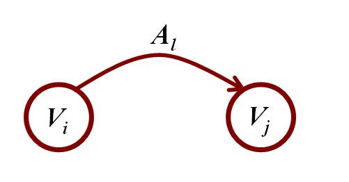
The problem that we are interested in is to understand which sets of Lyapunov inequalities imply stability of the switched system in (2). We will answer this question based on the corresponding graph.
For reasons that will become clear shortly, we would like to reduce graphs whose edges have arbitrary labels from the set to graphs whose edges have labels from the set , i.e., labels of length one. This is explained next.
Definition 1.
Given a labeled directed graph , we define its expanded graph as the outcome of the following procedure. For every edge with label , where , we remove the edge and replace it with new edges , where and .33 3 It is understood that the node index depends on the original nodes and . To keep the notation simple we write instead of . (These new edges go from node through newly added nodes and then to node .) We then label the new edges with respectively.

An example of a graph and its expansion is given in Figure 2. Note that if a graph has only labels of length one, then its expanded graph equals itself. The next definition is central to our development.
Definition 2.
Given a directed graph whose edges are labeled with words from the set , we say that the graph is path-complete, if for all finite words of any length (i.e., for all words in ), there is a directed path in its expanded graph such that the labels on the edges of this path are the labels up to .
In Figure 3, we present seven path-complete graphs on the alphabet . The fact that these graphs are path-complete is easy to see for graphs and , but perhaps not so obvious for graphs and . One way to check if a graph is path-complete is to think of it as a finite automaton by introducing an auxiliary start node (state) with free transitions to every node and by making all the other nodes be accepting states. Then, there are well-known algorithms (see e.g. [28, Chap. 4]) that check whether the language accepted by an automaton is , which is equivalent to the graph being path-complete. Similar algorithms exist in the symbolic dynamics literature; see e.g. [40, Chap. 3]. Our interest in path-complete graphs stems from Theorem 4 below that establishes that any such graph gives a method for approximation of the JSR. We introduce one last definition before we state this theorem.

Definition 3.
Let be a set of matrices. Given a path-complete graph and functions , we say that is a graph Lyapunov function (GLF) associated with if
where is the label associated with edge going from node to node .
Theorem 4.
Consider a finite set of matrices . For a scalar , let . Let be a path-complete graph whose edges are labeled with words from . If there exist positive, continuous, and homogeneous44 4 The requirement of homogeneity can be replaced by radial unboundedness which is implied by homogeneity and positivity. However, since the dynamical system in (2) is homogeneous, there is no conservatism in asking to be homogeneous. functions , one per node of the graph, such that is a graph Lyapunov function associated with , then .
Proof.
We will first prove the claim for the special case where the edge labels of belong to and therefore . The general case will be reduced to this case afterwards. Let be the degree of homogeneity of the Lyapunov functions , i.e., for all . (The actual value of is irrelevant.) By positivity, continuity, and homogeneity of , there exist scalars and with for , such that
| (9) |
for all and for all , where here denotes the Euclidean norm of . Let
| (10) |
Now consider an arbitrary product of length . Because the graph is path-complete, there will be a directed path corresponding to this product that consists of edges, and goes from some node to some node . If we write the chain of Lyapunov inequalities associated with these edges (cf. Figure 1), then we get
which by homogeneity of the Lyapunov functions can be rearranged to
| (11) |
We can now bound the spectral norm of as follows:
where the last three inequalities follow from (9), (11), and (10) respectively. From the definition of the JSR in (1), after taking the -th root and the limit , we get that and the claim is established.
Now consider the case where at least one edge of has a label of length more than one and hence 55 5 A reviewer kindly pointed out an alternative and shorter way of proving the second part of this theorem, without relying on the notion of expanded graphs. We present the proof with expanded graphs because the explicit relationship between the Lyapunov functions of a graph and its expanded version prove to be useful in showing equivalence of certain path-complete graphs in terms of the quality of approximation that they provide on the JSR. We will start with the Lyapunov functions assigned to the nodes of and from them we will explicitly construct Lyapunov functions for the nodes of that satisfy the Lyapunov inequalities associated to the edges in . Once this is done, in view of our preceding argument and the fact that the edges of have labels of length one by definition, the proof will be completed.
For , let us denote the new Lyapunov functions by . We give the construction for the case where The result for the general case follows by iterating this simple construction. Let be the added node in the expanded graph, and be such that and with and as the corresponding labels respectively. Define
| (12) |
By construction, and and subsequently, and are uniquely defined and hence, is well defined. We only need to show that
| (13) | ||||
| (14) |
Inequality (13) follows trivially from (12). Furthermore, it follows from (12) that
where the inequality follows from the fact that for , the functions satisfy the Lyapunov inequalities of the edges of ∎
Remark 2.1.
If the matrix is not invertible, the extended function as defined in (12) will only be positive semidefinite. However, since our goal is to approximate the JSR, we will never be concerned with invertibility of the matrices in . Indeed, since the JSR is continuous in the entries of the matrices [33, p. 18], we can always perturb the matrices slightly to make them invertible without changing the JSR by much. In particular, for any there exist such that
To understand the generality of the framework of “path-complete graph Lyapunov funcitons” more clearly, let us revisit the path-complete graphs in Figure 3 for the study of the case where the set consists of only two matrices. For all of these graphs if our choice for the Lyapunov functions or and are quadratic functions or sum of squares polynomial functions, then we can formulate the well-established semidefinite programs that search for these candidate Lyapunov functions.
Graph , which is clearly the simplest possible one, corresponds to the well-known common Lyapunov function approach. Graph is a common Lyapunov function applied to all products of length two. This graph also obviously implies stability.66 6 By slight abuse of terminology, we say that a graph implies stability meaning that the associated Lyapunov inequalities imply stability. But graph tells us that if we find a Lyapunov function that decreases whenever , , and are applied (but with no requirement when is applied), then we still get stability. This is a priori not obvious and we believe this approach has not appeared in the literature before. Graph is also an example that explains our reasoning behind the expansion process. Note that for the unexpanded graph, there is no path for any word of the form or of the form , for any However, one can check that in the expanded graph of graph , there is a path for every finite word, and this in turn allows us to conclude stability from the Lyapunov inequalities of graph .
The remaining graphs in Figure 3 which all have two nodes and four edges have a connection to the method of min-of-quadratics or max-of-quadratics Lyapunov functions [30], [29], [20], [31]. If Lyapunov inequalities associated with any of these four graphs are satisfied, then either or or both serve as a common Lyapunov function for the switched system. In the next section, we assert these facts in a more general setting (Corollaries 8 and 9) and show that these graphs in some sense belong to “simplest” families of path-complete graphs.
3 Duality and examples of families of path-complete graphs
Now that we have shown that any path-complete graph yields a method for proving stability of switched systems, our next focus is naturally on showing how one can produce graphs that are path-complete. Before we proceed to some basic constructions of such graphs, let us define a notion of duality among graphs which essentially doubles the number of path-complete graphs that we can generate.
Definition 5.
Given a directed graph whose edges are labeled with words in , we define its dual graph to be the graph obtained by reversing the direction of the edges of , and changing the labels of every edge of to its reversed version .

An example of a pair of dual graphs with labels of length one is given in Figure 4. The following theorem relates dual graphs and path-completeness.
Theorem 6.
If a graph is path-complete, then its dual graph is also path-complete.
Proof.
Consider an arbitrary finite word . By definition of path-completeness, our task is to show that there exists a path corresponding to this word in the expanded graph of the dual graph . It is easy to see that the expanded graph of the dual graph of is the same as the dual graph of the expanded graph of ; i.e, . Therefore, we show a path for in . Consider the reversed word . Since is path-complete, there is a path corresponding to this reversed word in . Now if we just trace this path backwards, we get exactly a path for the original word in . This completes the proof. ∎
The next proposition offers a very simple construction for obtaining a large family of path-complete graphs with labels of length one.
Proposition 7.
A graph having any of the two properties below is path-complete.
Property (i): every node has outgoing edges with all the labels in .
Property (ii): every node has incoming edges with all the labels in .
Proof.
If a graph has Property (i), then it is obviously path-complete. If a graph has Property (ii), then its dual has Property (i) and therefore by Theorem 6 it is path-complete. ∎
Examples of path-complete graphs that fall in the category of this proposition include graphs and in Figure 3 and all of their dual graphs. By combining the previous proposition with Theorem 4, we obtain the following two simple corollaries which unify several linear matrix inequalities (LMIs) that have been previously proposed in the literature. These corollaries also provide a link to min/max-of-quadratics Lyapunov functions. Different special cases of these LMIs have appeared in [30], [29], [20], [31], [36], [15], [38]. Note that the framework of path-complete graph Lyapunov functions makes the proof of the fact that these LMIs imply stability immediate. We also remark that the following corollaries, and hence the graphs in Proposition 7, already include infinite subsets of path-complete graphs that are not only sufficient for stability of (2), but also necessary. Examples of such infinite sets of LMIs with their proofs of necessity are given in [36], [38].
Corollary 8.
Proof.
The inequalities in (15) imply that every node of the associated graph has outgoing edges labeled with all the different matrices. Therefore, by Proposition 7 the graph is path-complete, and by Theorem 4 this implies absolute asymptotic stability. The proof that the pointwise minimum of the quadratics is a common Lyapunov function is easy and left to the reader. ∎
Corollary 9.
Proof.
The inequalities in (16) imply that every node of the associated graph has incoming edges labeled with all the different matrices. Therefore, by Proposition 7 the graph is path-complete and the proof of absolute asymptotic stability then follows. The proof that the pointwise maximum of the quadratics is a common Lyapunov function is again left to the reader. ∎
Remark 3.1.
The linear matrix inequalities in (15) and (16) are (convex) sufficient conditions for existence of min-of-quadratics or max-of-quadratics Lyapunov functions. The converse is not true. The works in [30], [29], [20], [31] have additional multipliers in (15) and (16) that make the inequalities non-convex but when solved with a heuristic method contain a larger family of min-of-quadratics and max-of-quadratics Lyapunov functions. Even if the non-convex inequalities with multipliers could be solved exactly, except for special cases where the -procedure is exact (e.g., the case of two quadratic functions), these methods still do not completely characterize min-of-quadratics and max-of-quadratics functions.
Remark 3.2.
The LMIs associated with “path-dependent quadratic Lyapunov functions” of any given path length (see [36]) and the LMIs associated with “parameter dependent Lyapunov functions” [15]—when specialized to the analysis of arbitrarily switched linear systems—are special cases of Corollary 8 and 9 respectively. This observation makes a connection between these techniques and min/max-of-quadratics Lyapunov functions which is not established in [36], [15]. It is also interesting to note that the path-complete graph corresponding to the LMIs of path-dependent quadratic Lyapunov functions of any path length (see Theorem 9 in [36]) is the well-known De Bruijn graph [23]. The “path length” of these Lyapunov functions is interestingly the dimension of the De Bruijn graph. We will analyze the bound on the JSR obtained by analysis via this path-complete graph in later sections since we have empirically observed that path-dependent quadratic Lyapunov functions are among the most powerful ones in comparison to all of our graphs.
The set of path-complete graphs is much broader than the family of graphs constructed in Proposition 7. Indeed, there are many graphs that are path-complete without having outgoing (or incoming) edges with all the labels on every node; see e.g. graph in Figure 5. This in turn means that there are several interesting and unexplored Lyapunov inequalities that we can impose for proving stability of switched systems. Below, we give one particular example of such “non-obvious” inequalities for the case of switching between two matrices.

Proposition 10.
Proof.
The graph associated with the LMIs above and its expanded version are drawn in Figure 5. We leave it as an exercise for the reader to show (e.g. by induction on the length of the word) that there is path for every finite word in . Therefore, is path-complete and in view of Theorem 4 the claim is established. ∎
Remark 3.3.
Proposition 10 can be generalized as follows: If a single Lyapunov function decreases with respect to the matrix products
for some integer , then . We omit the proof of this generalization due to space limitations. We will later prove (Theorem 18) a bound for the quality of approximation of path-complete graphs of this type, where a common Lyapunov function is required to decrease with respect to products of different lengths.
When we have so many different ways of imposing conditions for stability, it is natural to ask which ones are more powerful. The answer clearly depends on the combinatorial structure of the graphs and does not seem to be easy in general. Nevertheless, in the next section, we compare the performance of all path-complete graphs with two nodes for analysis of switched systems with two matrices. Some interesting connections between the bounds obtained from these graphs will arise. For example, we will see that the graphs and always give the same bound on the joint spectral radius; i.e., one graph will succeed in proving stability if and only if the other two will. So, there is no point in increasing the number of decision variables and the number of constraints and impose or in place of . The same is true for the graphs in and , which makes graph preferable to graph . (See Proposition 12.)
4 Path-complete graphs with two nodes
In this section, we characterize the set of all path-complete graphs consisting of two nodes, an alphabet set and edge labels of unit length. We will elaborate on the set of all admissible topologies arising in this setup and compare the performance—in the sense of conservatism of the ensuing analysis—of different path-complete graph topologies.
Before we proceed, we introduce a notation that will prove to be convenient in Subsection 4.2: Given a labeled graph associated with two matrices and , we denote by , the graph obtained by swapping of and in all the labels on every edge.
4.1 The set of path-complete graphs
The next lemma establishes that for thorough analysis of the case of two matrices and two nodes, we only need to examine graphs with four or fewer edges.
Lemma 11.
Let
be a path-complete graph with labels of length one for
. Let
be a graph Lyapunov function for If then, either
(i) there exists such that is a path-complete graph,
or
(ii) either or or both are common Lyapunov functions for
Proof.
If then at least one node has three or more outgoing edges. Without loss of generality let node be a node with exactly three outgoing edges , and let Let denote the destination node of an edge If then (or ) can be removed without changing the output set of words. If assume, without loss of generality, that and Now, if then regardless of its destination node, can be removed. If and , then is a common Lyapunov function for . The only remaining possibility is that and Note that there must be an edge from node to node , otherwise either node would have two self-edges with the same label or would be a common Lyapunov function for . If then it can be verified that is path-complete and thus all other edge can be removed. If there is no edge from node to node with label then and node must have a self-edge with label , otherwise the graph would not be path-complete. In this case, it can be verified that can be removed without affecting the output set of words. ∎
One can easily verify that a path-complete graph with two nodes and fewer than four edges must necessarily place two self-loops with different labels on one node, which necessitates existence of a common Lyapunov function for the underlying switched system. Since we are interested in exploiting the favorable properties of graph Lyapunov functions in approximation of the JSR, we will focus on graphs with four edges.
4.2 Comparison of performance
It can be verified that for path-complete graphs with two nodes, four edges, and two matrices, and without multiple self-loops on a single node, there are a total of nine distinct graph topologies to consider. Of the nine graphs, six have the property that every node has two incoming edges with different labels. These are graphs and (Figure 3). Note that and . The duals of these six graphs, i.e., and have the property that every node has two outgoing edges with different labels. Evidently, and are self-dual graphs, i.e., they are isomorphic to their dual graphs. The self-dual graphs are least interesting to us since, as we will show, they necessitate existence of a common Lyapunov function for (cf. Proposition 12, equation (18)).
Note that all of these graphs perform at least as well as a common Lyapunov function because we can always take . Furthermore, we know from Corollaries 9 and 8 that if Lyapunov inequalities associated with and are satisfied, then is a common Lyapunov function, whereas, in the case of graphs , and , the function would serve as a common Lyapunov function. Clearly, for the self-dual graphs and both and are common Lyapunov functions.
Notation: Given a set of matrices a path-complete graph and a class of functions we denote by the upper bound on the JSR of that can be obtained by numerical optimization of GLFs defined over With a slight abuse of notation, we denote by the upper bound that is obtained by using a common Lyapunov function
Proposition 12.
Consider the set and let , and be the path-complete graphs shown in Figure 3. Then, the upper bounds on the JSR of obtained via the associated GLFs satisfy the following relations:
| (17) |
and
| (18) |
and
| (19) |
and
| (20) |
Proof.
A proof of (17) in more generality is provided in Section 5 (cf. Corollary 15). The proof of (18) is based on symmetry arguments. Let be a GLF associated with ( is associated with node and is associated with node ). Then, by symmetry, is also a GLF for (where is associated with node and is associated with node ). Therefore, letting , we have that is a GLF for and thus, is also a common Lyapunov function for which implies that The other direction is trivial: If is a common Lyapunov function for then is a GLF associated with and hence, Identical arguments based on symmetry hold for and . We now prove the left equality in (19), the proofs for the remaining equalities in (19) and (20) are analogous. The equivalence between and is a special case of the relation between a graph and its reduced model, obtained by removing a node without any self-loops, adding a new edge per each pair of incoming and outgoing edges to that node, and then labeling the new edges by taking the composition of the labels of the corresponding incoming and outgoing edges in the original graph; see [47], [46, Chap. 5]. Note that is an offspring of in this sense. This intuition helps construct a proof. Let be a GLF associated with It can be verified that is a Lyapunov function associated with and therefore, Similarly, if is a Lyapunov function associated with then one can check that is a GLF associated with and hence, ∎

Remark 4.1.
The diagram in Figure 6 summarizes the results of this section. We remark that no relations other than the ones given in Figure 6 can be established among these path-complete graphs. Indeed, whenever there are no relations between two graphs in Figure 6, we have examples of matrices for which one graph can outperform the other. These examples are not presented here but are available online and can be retrieved from [1].
Based on our numerical experiments, the graphs and seem to statistically perform better than all other graphs in Figure 6. For example, we ran experiments on a set of random matrices with elements uniformly distributed in to compare the performance of graphs and . If in each case we also consider the relabeled matrices (i.e., ) as our input, then, out of the total instances, graph produced strictly better bounds on the JSR times, whereas graphs and each produced the best bound of the three graphs only times. (The numbers do not add up to due to ties.) In addition to this superior performance, the bound obtained by analysis via the graph is invariant under (i) permutation of the labels and (obvious), and (ii) transposing of and (Corollary 15). These are desirable properties which fail to hold for and or their duals. Motivated by these observations, we generalize and its dual in the next section to the case of matrices and Lyapunov functions and establish that they have certain appealing properties. We will prove (cf. Theorem 16) that these graphs always perform better than a common Lyapunov function in 2 steps (i.e., the graph in Figure 3), whereas, this is not the case for and or their duals.
5 Further analysis of a particular family of path-complete graphs
The framework of path-complete graphs provides a multitude of semidefinite programming based techniques for the approximation of the JSR whose performance vary with computational cost. For instance, as we increase the number of nodes of the graph, or the degree of the polynomial Lyapunov functions assigned to the nodes, or the number of edges of the graph that instead of labels of length one have labels of higher length, we obtain better results but at a higher computational cost. Many of these approximation techniques are asymptotically tight, so in theory they can be used to achieve any desired accuracy of approximation. For example,
where denotes the class of sum of squares homogeneous polynomial Lyapunov functions of degree . (Recall our notation for bounds from Section 4.2.) It is also true that a common quadratic Lyapunov function for products of higher length achieves the true JSR asymptotically [9], [33]; i.e.77 7 By we denote the class of quadratic homogeneous polynomials. We drop the superscript “SOS” because nonnegative quadratic polynomials are always sums of squares.,
Nevertheless, it is desirable for practical purposes to identify a class of path-complete graphs that provide a good tradeoff between quality of approximation and computational cost. Towards this objective, we propose the use of quadratic Lyapunov functions assigned to the nodes of the De Bruijn graph88 8 The De Bruijn graph of dimension on symbols is a labeled directed graph with nodes and edges whose nodes are indexed by all possible words of length from the alphabet , and whose edges have labels of length one and are obtained by the following simple rule: There is an edge labeled with the letter (or for our purposes the matrix ) going from node to node , and . of dimension on symbols for the approximation of the JSR of a set of matrices. This is precisely the graph of path-dependent quadratic Lyapunov functions of path length [36]. This graph and its dual are particular path-complete graphs with nodes and edges and will be the subject of study in this section. If we denote the quadratic Lyapunov functions by , then we are proposing the use of linear matrix inequalities
| (21) |
or the set of LMIs
| (22) |
for the approximation of the JSR of matrices. We note that the LMIs in (21) have appeared in [15, 38] and those in (22) have appeared in [36]. Throughout this section, we denote the path-complete graphs associated with (21) and (22) with and respectively. (The De Bruijn graph of dimension , by standard convention, is actually the graph .) Observe that and are indeed dual graphs as they can be obtained from each other by reversing the direction of the edges. For the case , our notation is consistent with the previous section and these graphs are illustrated in Figure 4. Also observe from Corollary 8 and Corollary 9 that the LMIs in (21) give rise to max-of-quadratics Lyapunov functions, whereas the LMIs in (22) lead to min-of-quadratics Lyapunov functions. We will prove in this section that the approximation bound obtained by these LMIs (i.e., the reciprocal of the largest for which the LMIs (21) or (22) hold) is always the same and lies within a multiplicative factor of of the true JSR, where is the dimension of the matrices. The relation between the bound obtained by a pair of dual path-complete graphs has a connection to transposition of the matrices in the set . We explain this next.
5.1 Duality and invariance under transposition
In [19], [20], it is shown that absolute asymptotic stability of the linear difference inclusion in (3) defined by the matrices is equivalent to absolute asymptotic stability of (3) for the transposed matrices . Note that this fact is immediately seen from the definition of the JSR in (1), since . It is also well-known that
Indeed, if is a common quadratic Lyapunov function for the set , then it is easy to show that is a common quadratic Lyapunov function for the set . However, this nice property is not true for the bound obtained from some other techniques. For instance, the next example shows that
| (23) |
i.e., the upper bound obtained by searching for a common quartic SOS polynomial is not invariant under transposition.
Example 5.1.
Consider the set of matrices with
We have but (up to three significant digits). This phenomenon is not due to the SOS relaxation and should be attributed to common quartic polynomial Lyapunov functions more generally. We know this because all five polynomial nonnegativity conditions in this problem (on the Lyapunov function and its decrements w.r.t. the four matrices) are imposed on ternary quartic forms. It is known from an old result of Hilbert [27] that all nonnegative ternary quartic forms are SOS.
Similarly, the bound obtained by non-convex inequalities proposed in [19] is not invariant under transposing the matrices. For such methods, one would have to run the numerical optimization twice—once for the set and once for the set —and then pick the better bound of the two. We will show that by contrast, the bound obtained from the LMIs in (21) and (22) are invariant under transposing the matrices. Before we do that, let us prove a general result which states that for path-complete graphs with quadratic Lyapunov functions as nodes, transposing the matrices has the same effect as dualizing the graph. We are grateful to a reviewer who kindly made us aware that an independent and earlier proof of this fact for certain families of path-complete graphs appears in [38].
Theorem 13.
Let be a path-complete graph, and let be its dual graph. Then,
| (24) |
Proof.
For ease of notation, we prove the claim for the case where the edge labels of have length one. The proof of the general case is identical. Pick an arbitrary edge going from node to node and labeled with some matrix . By the application of the Schur complement we have
But this already establishes the claim since we see that and satisfy the LMI associated with edge when the matrix is transposed if and only if and satisfy the LMI associated with edge . ∎
Corollary 14.
if and only if .
Proof.
This is an immediate consequence of the equality in (24). ∎
It is an interesting question for future research to characterize the path-complete graphs for which one has For example, the above corollary shows that this is obviously the case for any path-complete graph that is self-dual. Let us show next that this is also the case for graphs and despite the fact that they are not self-dual.
Corollary 15.
Proof.
The proof of (25) is established by observing that the GLFs associated with and can be derived from one another via (Note that we are relying here on the assumption that the matrices are invertible, which as we noted in Remark 2.1, is not a limiting assumption.) Since (25) in particular implies that , we get the rest of the equalities in (26) immediately from Corollary 14 and this finishes the proof. For concreteness, let us also prove the leftmost equality in (26) directly. Let , satisfy the LMIs in (21) for the set of matrices . Then, the reader can check that
satisfy the LMIs in (21) for the set of matrices . ∎
5.2 An approximation guarantee
The next theorem gives a bound on the quality of approximation of the estimate resulting from the LMIs in (21) and (22). Since we have already shown that it is enough to prove this bound for the LMIs in (21).
Theorem 16.
Let be a set of matrices in with JSR . Let be the bound on the JSR obtained from the LMIs in (21). Then,
| (27) |
Proof.
The right inequality is just a consequence of being a path-complete graph (Theorem 4). To prove the left inequality, consider the set consisting of all products of length two. In view of (6), a common quadratic Lyapunov function for this set satisfies the bound
It is easy to show that
See e.g. [33]. Therefore,
| (28) |
Now suppose for some , is a common quadratic Lyapunov function for the matrices in ; i.e., it satisfies
Then, we leave it to the reader to check that
satisfy (21). Hence,
and in view of (28) the claim is established. ∎
Note that the bound in (27) is independent of the number of matrices. Moreover, we remark that this bound is tighter, in terms of its dependence on , than the known bounds for for any finite degree of the sum of squares polynomials. The reader can check that the bound in (7) goes asymptotically as . Numerical evidence suggests that the performance of both the bound obtained by sum of squares polynomials and the bound obtained by the LMIs in (21) and (22) is much better than the provable bounds in (7) and in Theorem 16. The problem of improving these bounds or establishing their tightness is open. It goes without saying that instead of quadratic functions, we can associate sum of squares polynomials to the nodes of and obtain a more powerful technique for which we can also prove better bounds with the exact same arguments.
5.3 Numerical examples and applications
In the proof of Theorem 16, we essentially showed that the bound obtained from LMIs in (21) is tighter than the bound obtained from a common quadratic applied to products of length two. Our first example shows that the LMIs in (21) can in fact do better than a common quadratic applied to products of any finite length. We remind the reader that these LMIs correspond to the dual of the De Bruijn graph of dimension one and appear in [15], [38].
Example 5.2.
Consider the set of matrices with
This is a benchmark set of matrices that has been studied in [7], [43], [6] because it gives the worst case approximation ratio of a common quadratic Lyapunov function. Indeed, it is easy to show that , but . Moreover, the bound obtained by a common quadratic function applied to the set is
which for no finite value of is exact. On the other hand, we show that the LMIs in (21) give the exact bound; i.e., . Due to the simple structure of and , we can even give an analytical expression for our Lyapunov functions. Given any , the LMIs in (21) with are feasible with
for any and
Example 5.3.
Consider the set of randomly generated matrices with
A lower bound on is . The upper approximations for that we computed for this example are as follows:
| (29) |
The bound matches the lower bound numerically and is most likely exact for this example. This bound is slightly better than . However, a simple calculation shows that the semidefinite program resulting in has 25 more decision variables than the one for . Also, the running time of the algorithm leading to is noticeably larger than the one leading to . In general, when the dimension of the matrices is large, it can often be cost-effective to increase the number of the nodes of our path-complete graphs but keep the degree of the polynomial Lyapunov functions assigned to its nodes relatively low. For example, a path-dependent quadratic Lyapunov function with path length (i.e. the De Bruijn of dimension ) also achieves the exact JSR by solving a system of LMIs with quadratic functions and constraints.
Example 5.4.
Consider the set of matrices with
A lower bound for is . Here are some upper approximations for this example computed via four methods:
| (30) |
This example is interesting because the graph (see Fig. 3) is the cheapest computational method among the four (e.g. it has only one unknown matrix variable and three constraints, versus one unknown and four constraints for two unknowns and four constraints for ), but yet it is the only method that gets the JSR exactly. This shows that the quality of the different methods depends on the particular set of matrices. In particular, the method corresponding to the graph which has not appeared in the literature to the best of our knowledge, can outperform other choices in many randomly generated examples. For this example, if we increase the degree of the common SOS Lyapunov function from to , or the path length of the path-dependent quadratic Lyapunov function from to , then these methods also get the JSR exactly though at a higher computational cost.
Example 5.5.
Consider the set of matrices with
A lower bound for is Here are three upper bounds computed for this example:
| (31) |
Once again, graph , which is an example of a new method, outperforms the other two methods even though it solves a smaller semidefinite program.
What is also interesting in the above example is that it is quite challenging to prove that in fact gives the exact JSR; i.e. it is hard to find a matching upper bound. This goal can be achieved for example by a common SOS Lyapunov function of degree , but not by one of degree or lower. Similarly, path dependent quadratic Lyapunov functions of path lengths , , , or fail to find the exact JSR. However, if we combine the SOS method with path-dependent Lyapunov functions (i.e. assign SOS Lyapunov functions to nodes of the De Bruijn graph), then the exact JSR can be achieved by “{path length, SOS degree} pairs” equal to or or .
If one works with quadratic Lyapunov functions only, then path dependent quadratic Lyapunov functions of path length succeed in getting the JSR exactly. The resulting semidefinite program has unknown Lyapunov functions (matrix variables) and LMIs. By using new path-complete graphs, we were able to get the JSR exactly with only unknown quadratic Lyapunov functions and LMIs. The graph that achieved this (not shown) consists of nodes and edges and is closely related to Remark 3.3. Each node of this graph has outgoing edges with exactly the same label going to the nodes of the graph. The labels on the outgoing edges of the different nodes are respectively . We leave it to the reader to check that this graph is path-complete.
Performance on application-motivated problems. In the remainder of this section, we consider computational problems that arise from three different application scenarios. In all of these applications, the underlying problems have been already shown by the existing literature to be related to the computation of the JSR of certain matrices. We thus focus on the computational aspects, and demonstrate the usefulness of the path-complete graph Lyapunov function framework in situations that arise from practical scenarios.

Before we proceed, we introduce two new graphs and which can be verified to be path-complete99 9 For brevity, we do not provide proofs of path-completeness.. The first graph, , is shown in Figure 7 and is obtained by associating each word in the set with a different node on a complete directed graph of order 3, in which all the outgoing edges from every node have the same label. The second graph, (not shown), is a complete directed graph of order 9, and is obtained by applying the same principle to the set1010 10 The words in this set correspond to paths of length two on . Finally, we will use to denote the De Bruijn graph of dimension . (The number of symbols of the De Bruijn graph will be clear from the context and always equal to the number of matrices whose JSR is under consideration.)
Example 5.6.
Application to Computation of the Number of Overlap-Free Words. It was shown in [34] that the problem of computation of the smallest exponent of growth of the number of overlap-free or repetition-free binary words (see, e.g. [8]) reduces to the computation of the JSR of two sparse matrices and in . These relatively large-size matrices are explicitly presented in [34, 24], and are not repeated here in the interest of brevity. More precisely, letting denote the number of overlap-free binary words of length , we have:
It was conjectured in [34] that This conjecture was recently proven in [24] via a variation of the complex polytope algorithm specialized to non-negative matrices. In Table 1 we report the results of numerical computation of upper bounds on using various path-complete graphs. The approximate solver times are also reported which correspond to the CPU time of a 2.5 Ghz PC running the solver SeDuMi [49] on MATLAB.
| solver time | ||
|---|---|---|
| 2.5259 | 0.25 sec | |
| 2.5223 | 0.16 sec | |
| 2.51793404 | 1.87 sec | |
| 2.51793404 | 1.05 sec | |
| 2.51793404 |
The graphs and indeed provide an exact (up to machine precision) numerical value of the JSR and the running time of the SDP associated with is only second. These computations show that the path-complete graph Lyapunov function framework can provide very efficient methods for computation of the JSR in situations of practical and theoretical interest.
| N=17 | N=19 | solver time | |
|---|---|---|---|
| 0.118781760 | 0.097472458 | 0.15 sec | |
| 0.097471788 | 0.36 sec | ||
| 0.097463499 | 0.46 sec | ||
| 0.097407530 | 0.37 sec | ||
| 0.097403543 | 0.77 sec | ||
| 0.097334910 | 0.75 sec | ||
| 0.097332287 | 1.12 sec | ||
| 0.097306933 | 9.66 sec | ||
| 0.097380084 | 0.60 sec | ||
| 0.097306828 | 3.70 sec | ||
| 0.118781760 | 0.0973017161111 11 This number is only a lower bound on the JSR, given by . We conjecture that it is equal to the true JSR. |
Example 5.7.
Application to Computation of the Euler Ternary Partition Function. The problem of computation of the smallest exponent of growth of the Euler ternary partition function [44] can be reduced to the problem of computation of the JSR of three matrices with binary 0 or 1 entries. Herein, we examine a special case reported in [24], where the complex polytope method is applied to provide the exact value of the JSR of three 7-by-7 matrices with 0 and 1 entries:
In this case, the path-complete DeBruijn graph of dimension 1 yields an upper bound on the JSR with great accuracy in a fraction of a second; we have , and the computation time is 0.15sec on a 2.5 Ghz PC.
Example 5.8.
Application to Continuity of Wavelet Functions. Daubechies’ wavelet functions are orthonormal functions with compact support on satisfying
where, is a positive integer and the coefficients , satisfy certain additional constraints [22, 33]. The problem of computation of the Hölder exponent of continuity of the wavelet functions [16] is closely related to the problem of computation of the JSR of two linear operators, see, e.g., [33, Chap. 5], [42] and [22]. Herein, we are interested in computation of the JSR of the associated matrices for values of The matrix pairs are of dimension and have been posted online in [2] along with annotated MATLAB code for their computation. We remark that the JSR of the associated pairs of matrices for odd values of , were first reported in [22], where it was shown (numerically) that
| (32) |
Our numerical analysis conforms with the results of [22] for and a single common quadratic Lyapunov function () provides the exact (up to machine precision) numerical value of the JSR. For brevity, we do not repeat here the numerical values of the JSR for , and instead present the numerical upper-bound on the JSR for two more values of , i.e., and . Table 2 summarizes1212 12 As before, the approximate solver times correspond to the CPU time of a 2.5 Ghz PC running SeDuMi [49] on MATLAB. our numerical analysis for and . For the pattern holds and a single common quadratic Lyapunov function provides the exact value of the JSR which also satisfies (32). Surprisingly, however, for this pattern breaks and not only (32) does not hold, but also a common quadratic Lyapunov function does not give the exact upper bound! The best upper bound we are providing is obtained by graph which has 9 nodes and 90 LMIs. To the best of our knowledge none of the methods in the existing literature provide a better upper bound at a comparable computation cost.
6 Converse Lyapunov theorems and approximation with arbitrary accuracy
It is well-known that existence of a Lyapunov function which is the pointwise maximum of quadratics is not only sufficient but also necessary for absolute asymptotic stability of (2) or (3); see e.g. [41]. This is perhaps an intuitive fact if we recall that switched systems of type (2) and (3) always admit a convex Lyapunov function. Indeed, if we take “enough” quadratics, the convex and compact unit sublevel set of a convex Lyapunov function can be approximated arbitrarily well with sublevel sets of max-of-quadratics Lyapunov functions, which are intersections of ellipsoids. This of course implies that the bound obtained from max-of-quadratics Lyapunov functions is asymptotically tight for the approximation of the JSR. However, this converse Lyapunov theorem does not answer two natural questions of importance in practice: (i) How many quadratic functions do we need to achieve a desired quality of approximation? (ii) Can we search for these quadratic functions via semidefinite programming or do we need to resort to non-convex formulations? The same questions can naturally be asked for min-of-quadratics Lyapunov functions. The theorem and remark that follow provide an answer to these questions by relying on the connections that we have already established between min/max-quadratics Lyapunov functions and path-dependent Lyapunov functions [36] and their duals [38]. Our results further provides a worst case approximation guarantee for path-dependent quadratic Lyapunov functions of any given path length, and similarly for their duals.
Theorem 17.
Let be a set of matrices in . Given any positive integer , there exists an explicit path-complete graph consisting of nodes assigned to quadratic Lyapunov functions and edges with labels of length one such that the linear matrix inequalities associated with imply existence of a max-of-quadratics Lyapunov function and the resulting bound obtained from the LMIs satisfies
| (33) |
Proof.
Let us denote the quadratic Lyapunov functions by , where is a multi-index used for ease of reference to our Lyapunov functions. We claim that we can let be the graph dual to the De Bruijn graph of dimension on symbols. The LMIs associated to this graph are given by
| (34) |
These LMIs appear in [38] and are known to be asymptotically exact. The fact that is path-complete and that the LMIs imply existence of a max-of-quadratics Lyapunov function follows from Corollary 9. The proof that these LMIs satisfy the bound in (33) is a straightforward generalization of the proof of Theorem 16. By the same arguments we have
| (35) |
Suppose is a common quadratic Lyapunov function for the matrices in ; i.e., it satisfies
Then, it is easy to check that1313 13 The construction of the Lyapunov function here is a special case of a general scheme for constructing Lyapunov functions that are monotonically decreasing from those that decrease only every few steps; see [3, p. 58].
satisfy (34). Hence,
and in view of (35) the claim is established. ∎
Remark 6.1.
Arbitrarily good approximation bounds identical to those in Theorem 17 can be proven for min-of-quadratics Lyapunov functions in a similar fashion. The only difference is that the LMIs in (34) would get replaced by the ones corresponding to the dual graph of , i.e., the De Bruijn graph which is associated with path-dependent Lyapunov functions [36].
Our last theorem establishes approximation bounds for a family of path-complete graphs with one single node but several edges labeled with words of different lengths. Examples of such path-complete graphs include graph in Figure 3 and graph in Figure 5.
Theorem 18.
Let be a set of matrices in Let be a path-complete graph, and be the length of the shortest word in Then provides an estimate of that satisfies
Proof.
The right inequality is obvious, we prove the left one. Since both and are homogeneous in we may assume, without loss of generality, that . Suppose for the sake of contradiction that
| (36) |
We will show that this implies that . Towards this goal, let us first prove that Indeed, if we had , then there would exist1414 14 Here, we are appealing to the well-known fact about the JSR of a general set of matrices : See e.g. [33, Chap. 1]. an integer and a product such that
| (37) |
Since we also have (for some ), it follows that
| (38) |
The inequality in (37) together with gives
But this contradicts (38). Hence we have shown
Now, by our hypothesis (36) above, we have that Therefore, there exists such that It then follows from (6) that there exists a common quadratic Lyapunov function for Hence, which immediately implies that a contradiction. ∎
A noteworthy immediate corollary of Theorem 18 (obtained by setting is the following: If , then there exists a quadratic Lyapunov function that decreases simultaneously for all products of lengths , for any desired value of . Note that this fact is obvious for , but nonobvious for .
7 Conclusions and future directions
We introduced the framework of path-complete graph Lyapunov functions for the formulation of semidefinite programming based algorithms for approximating the joint spectral radius (or equivalently establishing absolute asymptotic stability of an arbitrarily switched linear system). We defined the notion of a path-complete graph, which was inspired by concepts in automata theory. We showed that every path-complete graph gives rise to a technique for the approximation of the JSR. This provided a unifying framework that includes many of the previously proposed techniques and also introduces new ones. (In fact, all families of LMIs that we are aware of are particular cases of our method.) We shall also emphasize that although we focused on switched linear systems because of our interest in the JSR, the analysis technique of multiple Lyapunov functions on path-complete graphs is clearly valid for switched nonlinear systems as well.
We compared the quality of the bound obtained from certain classes of path-complete graphs, including all path-complete graphs with two nodes on an alphabet of two matrices, and also a certain family of dual path-complete graphs. Among the different path-complete graphs considered in this paper, we observed that the De Bruijn graph and its dual, whose LMIs appear in the earlier work [36], [38], have a superior performance on average (but not always). Motivated by this fact, we studied these graphs in further detail. For example, we showed that stability analysis via these graphs is invariant under transposition of the matrices, results in common min/max-of-quadratics Lyapunov functions, and produces upper bounds on the JSR that are always within a multiplicative factor of of the true value, already for the first level of the hierarchy. Finally, we presented two converse Lyapunov theorems, one for the well-known methods of minimum and maximum-of-quadratics Lyapunov functions, and the other for a new class of methods that propose the use of a common quadratic Lyapunov function for a set of words of possibly different lengths.
We believe the methodology proposed in this paper should straightforwardly extend to the case of constrained switching by requiring the graphs to have a path not for all the words, but only the words allowed by the constraints on the switching. A rigorous treatment of this idea is left for future work.
Another question for future research is to determine the complexity of checking path-completeness of a given graph . As we explained in Section 2, well-known algorithms in automata theory (see e.g. [28, Chap. 4]) can check for path-completeness by testing whether the associated finite automaton accepts all finite words. When the automata are deterministic (i.e., when all outgoing edges from every node have different labels), these algorithms are very efficient and have running time of only . However, the problem of deciding whether a non-deterministic finite automaton accepts all finite words is known to be PSPACE-complete [18, p. 265]. Of course, the step of checking path-completeness of a graph is done offline and prior to the run of our algorithms for approximating the JSR. Therefore, while checking path-completeness is in general difficult, the approximation algorithms that we presented indeed run in polynomial time since they work with a fixed (a priori chosen) path-complete graph. Nevertheless, the question on complexity of checking path-completeness is interesting in many other settings, e.g., when deciding whether a given set of Lyapunov inequalities imply stability of an arbitrarily switched system.
Some other interesting questions that can be explored in the future are the following. What are some other classes of path-complete graphs that lead to new techniques for proving stability of switched systems? Can we classify graph operations that preserve path-completeness? How can we compare the performance of different path-complete graphs in a systematic way? Given a set of matrices, a class of Lyapunov functions, and a fixed size for the graph, can we efficiently come up with the least conservative topology of a path-complete graph? What properties of a set of matrices make a particular path-complete graph Lyapunov function better than another one? What are the analogues of the results of this paper for continuous time switched systems? To what extent do the results carry over to the synthesis (controller design) problem for switched systems? These questions and several others show potential for much follow-up work on path-complete graph Lyapunov functions.
References
- [1] URL: http://perso.uclouvain.be/raphael.jungers/contents/LMI_comparisons.txt.
- [2] URL: http://perso.uclouvain.be/raphael.jungers/contents/wavelets.zip.
- [3] A. A. Ahmadi. Non-monotonic Lyapunov functions for stability of nonlinear and switched systems: theory and computation. Master’s Thesis, Massachusetts Institute of Technology, June 2008. Available from http://dspace.mit.edu/handle/1721.1/44206.
- [4] A. A. Ahmadi, R. Jungers, P. A. Parrilo, and M. Roozbehani. Analysis of the joint spectral radius via Lyapunov functions on path-complete graphs. In Hybrid Systems: Computation and Control 2011, Lecture Notes in Computer Science. Springer, 2011.
- [5] A. A. Ahmadi, R. M. Jungers, P. A. Parrilo, and M. Roozbehani. When is a set of LMIs a sufficient condition for stability? arXiv preprint arXiv:1201.3227, 2012.
- [6] A. A. Ahmadi and P. A. Parrilo. Non-monotonic Lyapunov functions for stability of discrete time nonlinear and switched systems. In Proceedings of the 47th IEEE Conference on Decision and Control, 2008.
- [7] T. Ando and M.-H. Shih. Simultaneous contractibility. SIAM Journal on Matrix Analysis and Applications, 19:487–498, 1998.
- [8] J. Berstel. Growth of repetition-free wordsÑa review. Theoretical Computer Science, 340(2):280–290, 2005.
- [9] P. Bliman and G. Ferrari-Trecate. Stability analysis of discrete-time switched systems through Lyapunov functions with nonminimal state. In Proceedings of IFAC Conference on the Analysis and Design of Hybrid Systems, pages 325–330, 2003.
- [10] V. D. Blondel and Y. Nesterov. Computationally efficient approximations of the joint spectral radius. SIAM J. Matrix Anal. Appl., 27(1):256–272, 2005.
- [11] V. D. Blondel, Y. Nesterov, and J. Theys. On the accuracy of the ellipsoidal norm approximation of the joint spectral radius. Linear Algebra and its Applications, 394:91–107, 2005.
- [12] V. D. Blondel and J. N. Tsitsiklis. The boundedness of all products of a pair of matrices is undecidable. Systems and Control Letters, 41:135–140, 2000.
- [13] M. S. Branicky. Multiple Lyapunov functions and other analysis tools for switched and hybrid systems. IEEE Transactions on Automatic Control, 43(4):475–482, 1998.
- [14] C. T. Chang and V. D. Blondel. An experimental study of approximation algorithms for the joint spectral radius. Numerical Algorithms, pages 1–22, 2012.
- [15] J. Daafouz and J. Bernussou. Parameter dependent Lyapunov functions for discrete time systems with time varying parametric uncertainties. Systems and Control Letters, 43(5):355–359, 2001.
- [16] I. Daubechies and J. C. Lagarias. Two-scale difference equations ii. local regularity, infinite products of matrices and fractals. SIAM Journal on Mathematical Analysis, 23(4):1031–1079, 1992.
- [17] J. M. H. G. Vankeerberghen and R. M. Jungers. The JSR toolbox. Matlab Central, http://www.mathworks.com/matlabcentral/fileexchange/33202-the-jsr-toolbox.
- [18] M. R. Garey and D. S. Johnson. Computers and Intractability. W. H. Freeman and Co., San Francisco, Calif., 1979.
- [19] R. Goebel, T. Hu, and A. R. Teel. Dual matrix inequalities in stability and performance analysis of linear differential/difference inclusions. In Current Trends in Nonlinear Systems and Control, pages 103–122. 2006.
- [20] R. Goebel, A. R. Teel, T. Hu, and Z. Lin. Conjugate convex Lyapunov functions for dual linear differential inclusions. IEEE Transactions on Automatic Control, 51(4):661–666, 2006.
- [21] G. Gripenberg. Computing the joint spectral radius. Linear Algebra and its Applications, 234:43–60, 1996.
- [22] G. Gripenberg. Computing the joint spectral radius. Linear Algebra and its Applications, 234:43–60, 1996.
- [23] J. L. Gross and J. Yellen. Handbook of Graph Theory (Discrete Mathematics and Its Applications). CRC Press, 2003.
- [24] N. Guglielmi and V. Protasov. Exact computation of joint spectral characteristics of linear operators. Foundations of Computational Mathematics, 13(1):37–97, 2013.
- [25] N. Guglielmi and M. Zennaro. An algorithm for finding extremal polytope norms of matrix families. Linear Algebra and its Applications, 428:2265–2282, 2008.
- [26] N. Guglielmi and M. Zennaro. Finding extremal complex polytope norms for families of real matrices. SIAM Journal on Matrix Analysis and Applications, 31(2):602–620, 2009.
- [27] D. Hilbert. Über die Darstellung Definiter Formen als Summe von Formenquadraten. Math. Ann., 32, 1888.
- [28] J. E. Hopcroft, R. Motwani, and J. D. Ullman. Introduction to Automata Theory, Languages, and Computation. Addison Wesley, 2001.
- [29] T. Hu and Z. Lin. Absolute stability analysis of discrete-time systems with composite quadratic Lyapunov functions. IEEE Transactions on Automatic Control, 50(6):781–797, 2005.
- [30] T. Hu, L. Ma, and Z. Li. On several composite quadratic Lyapunov functions for switched systems. In Proceedings of the 45th IEEE Conference on Decision and Control, 2006.
- [31] T. Hu, L. Ma, and Z. Lin. Stabilization of switched systems via composite quadratic functions. IEEE Transactions on Automatic Control, 53(11):2571 – 2585, 2008.
- [32] M. Johansson and A. Rantzer. Computation of piecewise quadratic Lyapunov functions for hybrid systems. IEEE Transactions on Automatic Control, 43(4):555–559, 1998.
- [33] R. Jungers. The joint spectral radius: theory and applications, volume 385 of Lecture Notes in Control and Information Sciences. Springer, 2009.
- [34] R. M. Jungers, V. Y. Protasov, and V. D. Blondel. Overlap-free words and spectra of matrices. Theoretical Computer Science, 410(38):3670–3684, 2009.
- [35] J. W. Lee and G. E. Dullerud. Optimal disturbance attenuation for discrete-time switched and Markovian jump linear systems. SIAM Journal on Control and Optimization, 45(4):1329–1358, 2006.
- [36] J. W. Lee and G. E. Dullerud. Uniform stabilization of discrete-time switched and Markovian jump linear systems. Automatica, 42(2):205–218, 2006.
- [37] J. W. Lee and P. P. Khargonekar. Optimal output regulation for discrete-time switched and Markovian jump linear systems. SIAM Journal on Control and Optimization, 47(1):40–72, 2008.
- [38] J. W. Lee and P. P. Khargonekar. Detectability and stabilizability of discrete-time switched linear systems. IEEE Transactions on Automatic Control, 54(3):424–437, 2009.
- [39] H. Lin and P. J. Antsaklis. Stability and stabilizability of switched linear systems: a short survey of recent results. In Proceedings of IEEE International Symposium on Intelligent Control, 2005.
- [40] D. Lind and B. Marcus. An Introduction to Symbolic Dynamics and Coding. Cambridge University Press, 1995.
- [41] A. Molchanov and Y. Pyatnitskiy. Criteria of asymptotic stability of differential and difference inclusions encountered in control theory. Systems and Control Letters, 13:59–64, 1989.
- [42] I. I. Novikov, V. I. Protasov, and M. A. Skopina. Wavelet Theory, volume 239. AMS Bookstore, 2011.
- [43] P. A. Parrilo and A. Jadbabaie. Approximation of the joint spectral radius using sum of squares. Linear Algebra and its Applications, 428(10):2385–2402, 2008.
- [44] V. Y. Protasov. Asymptotic behaviour of the partition function. Sbornik: Mathematics, 191(3):381, 2000.
- [45] V. Y. Protasov, R. M. Jungers, and V. D. Blondel. Joint spectral characteristics of matrices: a conic programming approach. SIAM Journal on Matrix Analysis and Applications, 31(4):2146–2162, 2010.
- [46] M. Roozbehani. Optimization of Lyapunov invariants in analysis and implementation of safety-critical software systems. PhD thesis, Massachusetts Institute of Technology, 2008.
- [47] M. Roozbehani, A. Megretski, E. Frazzoli, and E. Feron. Distributed Lyapunov functions in analysis of graph models of software. Springer Lecture Notes in Computer Science, 4981:443–456, 2008.
- [48] G. C. Rota and W. G. Strang. A note on the joint spectral radius. Indag. Math., 22:379–381, 1960.
- [49] J. F. Sturm. Using SeDuMi 1.02, a MATLAB toolbox for optimization over symmetric cones. Optimization Methods and Software, 11(12):625–653, 1999. URL: http://sedumi.ie.lehigh.edu/.
- [50] J. N. Tsitsiklis and V. Blondel. The Lyapunov exponent and joint spectral radius of pairs of matrices are hard- when not impossible- to compute and to approximate. Mathematics of Control, Signals, and Systems, 10:31–40, 1997.