Spin interfaces in the Ashkin-Teller model and SLE

The scaling limit of interfaces in statistical models has attracted much attention since the early developments of conformal field theory (CFT). Starting from a local, classical spin model – e.g. the ${\rm O}(n)$, Potts, $\mathbb{Z}_{N}$, XY models – there are essentially two ways of defining extended interfaces. One may consider the polygons in a graphical high-temperature expansion, or the spin interfaces (or domain walls) separating regions with different spin values.

As far as exact solutions are concerned, the situation turns out to be very different for these two kinds of interfaces. On one hand, in several models, including the ${\rm O}(n)$ and Potts models, the high-temperature polygons are described by a Coulomb gas (CG) [1, 2], i.e. in the scaling limit, they become the level lines of a free compact boson CFT. Many geometric properties of these polygons can then be computed exactly through their mapping to correlation functions in this CFT. This yielded also solid conjectures (and, in some cases, rigorous proofs [3]) about their convergence to a Schramm-Loewner Evolution (SLE) model. On the other hand, despite some recent progress [4, 5], no consistent theory was identified as the scaling limit of spin interfaces, even in well-studied models such as the Potts model (except in the particular case of the Ising model), and very few scaling properties of these interfaces are actually known analytically.

Another current research direction is the study of “extended” SLEs, which are curve models determined by two random processes: the driving process of the Loewner chain, and an additional process corresponding, in the associated statistical model, to local variables which are not fixed locally by the presence of the curve. It was argued [6, 7] that the martingale conditions for this pair of processes correspond to null-state equations in an extended CFT. In particular, the presence of the additional process affects the relation between the central charge $c$ and the SLE parameter $\kappa$. An important point that needs to be considered in this context, is that in the presence of additional variables, the lattice interface no longer satisfies the Markov property, which is an essential ingredient of the SLE model.

The Ashkin-Teller (AT) model is a simple local spin model, with a critical line of constant central charge $c=1$ and varying exponents. We believe it presents the two features described above: first, although it has been much studied with both lattice and CFT techniques, the scaling theory for its spin interfaces is not identified, and second, these interfaces leave some fluctuating variables, which makes them good candidates for extended SLEs.

This paper presents two advances in the study of spin interfaces, on the particular example of the AT model. First, we introduce some specific boundary conditions (BCs) which ensure that the spin interface satisfies the Markov property, even in the presence of an additional variable. We then verify numerically that our interface relates to SLE, and for this purpose, we introduce a new algorithm allowing the measurement of the left-passage probability [8] in the transfer-matrix formalism. Our results also include an accurate numerical determination of the fractal dimension $d_{f}$ of spin interfaces, also by means of the transfer matrix, which supports a conjecture for $d_{f}$ stated in [9]. Second, we identify a specific value on the critical line of the AT model, where the temperature tends to zero, and at this point, we describe an exact mapping of the AT model onto an integrable 19-vertex model. Although this second result does not give direct access to spin interface exponents, this represents an alternative way of solving exactly the AT model, and may lead to additional exact results on this model.

The Ashkin-Teller model is a two-parameter model with a self-dual, critical line along which the central charge is constant $c=1$ and the critical exponents vary. Its local correlation functions are described by the $\mathbb{Z}_{2}$-orbifold of the compact boson CFT. However, like for the Potts model, this CG description only yields results for a specific class of interfaces, which does not include the spin DWs. A striking fact illustrating this is the absence of an exact result (except at specific values of the couplings) for the fractal dimension of spin DWs along the critical line!

To be more precise, let us summarize here the current knowledge on spin interfaces in the AT model. On the square lattice, the AT model consists of two spin variables $\sigma_{j}$ and $\tau_{j}$ at each site $j$, taking the values $\pm 1$, and with the Boltzmann weight

$$W[\sigma,\tau]=\prod_{\langle ij\rangle}\exp\left[\beta(\sigma_{i}\sigma_{j}+\tau_{i}\tau_{j})+\alpha\ \sigma_{i}\sigma_{j}\ \tau_{i}\tau_{j}\right]\,,$$

(1)

where the product is on all pairs of neighbouring sites. The critical line for the square lattice is given by the condition:

$$\sinh 2\beta=e^{-2\alpha}\,,$$

(2)

which we parametrize as

$$2-{\rm\coth}\ 2\beta=1-e^{4\alpha}=2\cos\pi g\,,\qquad\text{with $0\leq g\leq 1$.}$$

(3)

To exhibit the $\mathbb{Z}_{4}$ invariance of the model, it is convenient to introduce the complex variables $S_{j}:=\frac{\sigma_{j}-i\tau_{j}}{1-i}$, satisfying $S_{j}^{4}=1$, so that one can write (1) as

$$W[S]=\prod_{\langle ij\rangle}\exp\left\{\beta(S_{i}^{*}S_{j}+S_{j}^{*}S_{i})+\frac{\alpha}{2}\ \left[(S_{i}^{*}S_{j})^{2}+(S_{j}^{*}S_{i})^{2}\right]\right\}\,.$$

(4)

This Boltzmann weight is invariant under the global rotation $S_{j}\to e^{\frac{i\pi}{2}}S_{j}$ and reflection $S_{j}\to S_{j}^{*}$. A non-branching spin interface in the AT model is specified by the partition into two sets of the four possible spin configurations $(\sigma,\tau)$:

$$1:(++)\qquad 2:(+-)\qquad 3:(--)\qquad 4:(-+)\,.$$

(5)

For example, $(14|23)$ denotes the interface between sites with values $1$ or $4$, and sites with values $2$ or $3$. The symmetries of (4) only leave three possible nonequivalent non-branching spin interfaces:

• •

  The case $(13|24)$ corresponds to domain walls for the variable $\tau^{\prime}=\sigma\tau$. The associated operator has constant conformal dimension $h=\frac{1}{4}$ throughout the critical line, and hence the fractal dimension is $\frac{3}{2}$. In a previous work [10], we constructed a discrete holomorphic parafermion $\psi_{s}$ of spin $s$ in the AT model, which allowed us to relate the $(13|24)$ interface to $\rm SLE(4,\rho,\rho)$, where the value of $\rho$ was derived from the knowledge of $s$. The problem of the $(13|24)$ interface with various boundary conditions was also addressed numerically in [11] and [12], yielding a set of conjectured relations to $\rm SLE(4,\rho^{\prime},\rho^{\prime})$, and confirming the above results.

• •

  The case $(1|234)$ is not understood for general couplings, but for $g=3/4$ (where the AT model coincides with the integrable Fateev-Zamolodchikov $\mathbb{Z}_{4}$ spin model), the associated operator satisfies a null-state equation in the $\mathbb{Z}_{4}$-parafermionic CFT, and is argued [13] to have fractal dimension $\frac{17}{12}$.

• •

  The case $(12|34)$ corresponds to domain walls for the variable $\sigma$. Its fractal dimension is only known for a few values of the parameter $g$:

  $g$	univ. class	$d_{f}$
  $1/4$	${\rm O}(n=2)$	${3}/{2}$
  $1/2$	Ising	${11}/{8}$
  $3/4$	$\mathbb{Z}_{4}$-parafermions	${17}/{12}$
  $1$	four-state Potts	${3}/{2}$

  The fractal dimension cannot be simply obtained from the CG analysis. However, based on the above exact values and Monte-Carlo simulations (in the region between Ising and Potts points), the following expression was proposed [9] for $d_{f}$:

  $$d_{f}=\frac{7}{8}+\frac{g}{2}+\frac{1}{8g}\,.$$

  (6)

The value $g=1/3$ on the self-dual line (3) corresponds to the limit

$$\alpha\to-\infty,\qquad\beta\to\infty,\qquad e^{\alpha+\beta}=\sqrt{2}\,.$$

The Boltzmann weights then take the form

$$e^{-(2\beta+\alpha){\cal N}}\ W[\sigma,\tau]=\prod_{\langle ij\rangle}\left[\delta_{\sigma_{i},\sigma_{j}}\ \delta_{\tau_{i},\tau_{j}}+\frac{1}{2}\delta_{\sigma_{i},\sigma_{j}}\ (1-\delta_{\tau_{i},\tau_{j}})+\frac{1}{2}(1-\delta_{\sigma_{i},\sigma_{j}})\ \delta_{\tau_{i},\tau_{j}}\right]\,,$$

(12)

where $\cal N$ is the number of edges in $\Omega$. The corresponding $\sigma$ and $\tau$ domain walls thus form a two-colour loop model on the dual lattice, where a black (resp. gray) loop represents a $\sigma$ (resp. $\tau$) domain wall. Each edge of the dual lattice bears at most one colour of loop, and the weight of a loop configuration is $K^{\ell}$, where $K=1/2$, and $\ell$ is the total length of the loops. For completeness, we depict in Fig. 4 all the possible loop configurations around a vertex.

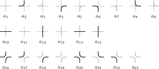
Let us now expose an exact equivalence of this two-colour loop model of AT spin interfaces with an integrable 19-vertex (19V) model. As a first stage, we map the 19V model onto a dilute Brauer model with loop weight $n=2$. The vertices of the latter model are shown in Fig. 5. Each of the Brauer loops can be oriented clockwise or anti-clockwise independently: this leads to a 19V model with weights

	$\displaystyle\omega_{1}$	$\displaystyle=$	$\displaystyle t$		(13)
	$\displaystyle\omega_{2}=\omega_{3}=\omega_{4}=\omega_{5}$	$\displaystyle=$	$\displaystyle u_{1}$		(14)
	$\displaystyle\omega_{6}=\omega_{7}=\omega_{8}=\omega_{9}$	$\displaystyle=$	$\displaystyle u_{2}$		(15)
	$\displaystyle\omega_{10}=\omega_{11}=\omega_{12}=\omega_{13}$	$\displaystyle=$	$\displaystyle v$		(16)
	$\displaystyle\omega_{14}=\omega_{15}$	$\displaystyle=$	$\displaystyle w_{1}+x$		(17)
	$\displaystyle\omega_{16}=\omega_{17}$	$\displaystyle=$	$\displaystyle w_{2}+x$		(18)
	$\displaystyle\omega_{18}=\omega_{19}$	$\displaystyle=$	$\displaystyle w_{1}+w_{2}\,,$		(19)

where we have used the standard notations $(\omega_{1},\dots,\omega_{19})$ as in [14]. If we take the FZ integrable weights [14] of the 19V, we obtain the dilute Brauer weights:

$$\begin{array}[]{rcl}t&=&\sin\mu\sin 2\mu-\sin u\sin(\mu-u)\\ u_{1}&=&\sin 2\mu\sin(\mu-u)\\ u_{2}&=&\sin 2\mu\sin u\\ v&=&\sin u\sin(\mu-u)\\ w_{1}&=&\sin 2\mu\sin(\mu-u)\cos u\\ w_{2}&=&\sin 2\mu\sin u\cos(\mu-u)\\ x&=&-\cos 2\mu\sin u\sin(\mu-u)\,.\end{array}$$

(20)

It turns out that setting $\mu=\frac{2\pi}{3}$ and $u=\mu/2$, and letting $v\to-v$ (because $v$ configurations always appear in even number) yields

$$\begin{array}[]{rcl}t&=&1\\ u_{1}=u_{2}=v&=&K\\ w_{1}=w_{2}&=&K^{2}\\ x&=&-K^{2}\,.\end{array}$$

(21)

The dilute Brauer model is, in turn, mapped to our two-colour loop model in the following way. Each of the Brauer loops can be coloured black or gray independently. Then, consider a vertex whose four adjacent edges bear the same colour. Since the coloured loops have weight unity, the overall Boltzmann weight of the configuration is the same for vertices $w_{1}$,$w_{2}$ and $x$. Thus the dilute Brauer model is equivalent to the two-colour loop model provided the following relations hold

$$\begin{array}[]{rcl}a_{1}&=&t\\ a_{2}=\dots=a_{5}&=&u_{1}\\ a_{6}=\dots=a_{9}&=&u_{2}\\ a_{10}=\dots=a_{13}&=&v\\ a_{14}=a_{15}&=&\pm x\\ a_{16}+a_{20}=w_{19}+w_{23}&=&w_{1}+w_{2}+x\\ a_{17}=a_{18}&=&w_{1}\\ a_{21}=a_{22}&=&w_{2}\end{array}$$

(22)

The integrable weights (21) satisfy these relations, and hence we have proved the equivalence.

For the parameters $\mu=\frac{2\pi}{3}$ and $u=\mu/2$, the 19V model is described [16] in the continuum limit by a $c=1$ compact boson CFT with the spectrum of conformal dimensions

$$x_{n,m}=\frac{\mu}{2\pi}n^{2}+\frac{\pi}{2\mu}m^{2}\,,\qquad n,m\in\mathbb{Z}^{2}\,.$$

(23)

It turns out that the excitations described by this spectrum describes are not directly related to those of the colored loops. In particular, they do not include the conjectured two-leg exponent $x_{2}=7/12$. However, the mapping to a 19V model may be exploited to obtain new exact results on the AT model at zero temperature.

In the present work, we have presented a set of new results on spin interfaces in the AT model.

By a numerical study based on transfer-matrix diagonalisation, we have given a precise numerical determination of the fractal dimension $d_{f}$, in a parameter regime that could not be accessed previously by a Monte-Carlo simulation [9]. Our results on $d_{f}$ bring more support to the conjectural expression (6) introduced in [9]. Moreover, we have shown, for the first time, how to adapt the transfer-matrix method to measure numerically the left-passage probability $P_{\rm left}$, which is a natural quantity in the SLE literature.

On the analytical side, we introduce a general way of choosing BCs which preserve the discrete Markov property of a path, even in the presence of additional degrees of freedom which are not fixed locally by the path. This construction is quite general, and may be extended to any lattice model with interfaces of this sort. The left-passage probability $P_{\rm left}$ is then computed numerically with these “Markovian” BCs, and the results for $P_{\rm left}$ confirm that the resulting measure on curves becomes SLE in the continuum limit.

We have also identified a specific point on the critical line of the AT model, the point where all the couplings diverge, where there is a mapping of the AT model onto an integrable 19-vertex model. At this point the interfaces of the $\sigma$ and $\tau$ spins live in different bonds and so the corresponding two-color loop model has a simpler form. At this particular point one can also find a dilute Brauer model representation of the critical spin interfaces of the AT model. Since the loop model has a simpler form at this particular point, we believe it is a good place to look for a Coulomb gas representation of the AT spin interfaces, and extend it to the critical line afterwards.

Our work presents conclusive numerical arguments that the spin interfaces in AT model are conformally invariant and their fractal dimension follow the formula (6), motivating further the search for an analytic argument which would account for (6). This is a simple example of the more general notion of spin interfaces, for which very few analytical results are available. On top of the recent methods for the study of lattice models, like discrete holomorphic parafermions, our construction of “Markovian” BCs seems an interesting starting point for this search.

In this Appendix, we present a numerical procedure for the computation of the left-passage probability in a loop model defined on the infinite strip of width $L$ sites. Let us describe how our method works on a simple loop model, such as the square-lattice ${\rm O}(n)$ loop model (defined by the vertices in Fig. 5, with $x=0$). The generalization to other loop models, such as the two-colour loop model studied in this paper, is straightforward.

The basis elements $\alpha$ generating the space of states $V_{L}$ are labelled by planar pairings of the points $\{1,\dots,L\}$, with one point paired with $\star$, as depicted in Fig. 6. The space $V_{L}$ is also equipped with a scalar product $\langle\cdot,\cdot\rangle$, defined as follows. We say that two pairings $\alpha,\beta$ are compatible if they have the same subset of paired points, and we denote $\bar{\alpha}\beta$ the figure obtained by gluing the $\pi$-rotation of $\alpha$ to $\beta$. Then

$$\langle\alpha,\beta\rangle:=\begin{cases}n^{\#{\rm closed\ loops\ in}\ \bar{\alpha}\beta}&\text{if $\alpha$ and $\beta$ are compatible,}\\ 0&\text{otherwise.}\end{cases}$$

(24)

Let us recall briefly how the transfer matrix $T$ acts on $V_{L}$ [15]. We take the convention that $T$ acts from bottom to top, and adds one row to the system. When starting from a pairing configuration $|\beta\rangle$, the addition of one row gives rise to a linear combination of pairings $\sum_{\alpha}T_{\alpha\beta}|\alpha\rangle$, where the matrix element $T_{\alpha\beta}$ is given by the product of Boltzmann weights inside the row, including a factor $n$ for each loop that got closed in the process.

We denote the dominant eigenstate of $T$ in the sector with a propagating path as

$$|\psi\rangle=\sum_{\alpha}\psi_{\alpha}|\alpha\rangle\,.$$

(25)

If we cut the system into two half-infinite strips above and below a given horizontal section, then the $L$ dangling edges of the top half have a pairing $\bar{\alpha}$, and those of the bottom half have a pairing $\beta$. If we assume that the local Boltzmann weights in $T$ are invariant under a rotation of angle $\pi$, then the probability of a pair $(\bar{\alpha},\beta)$ is

$$\mathbb{P}(\bar{\alpha},\beta)=\frac{\psi_{\alpha}\psi_{\beta}\langle\alpha,\beta\rangle}{Z}\,,\qquad\text{where}\qquad Z=\sum_{\alpha,\beta}\psi_{\alpha}\psi_{\beta}\langle\alpha,\beta\rangle$$

(26)

For any pair $(\bar{\alpha},\beta)$, we denote $\gamma_{\bar{\alpha},\beta}$ the open path appearing in $\bar{\alpha}\beta$. For a given position $j\in\{0,\dots,L\}$, we introduce the modified scalar product $\langle\cdot,\cdot\rangle_{j}$:

$$\langle\alpha,\beta\rangle_{j}:=\begin{cases}n^{\#{\rm closed\ loops\ in}\ \bar{\alpha}\beta}&\text{if $\alpha$ and $\beta$ are compatible and $\gamma_{\bar{\alpha},\beta}$ passes between $0$ and $j$,}\\ 0&\text{otherwise.}\end{cases}$$

(27)

This allows us to express the left-passage probability $P_{\rm left}$ as

$$P_{\rm left}(j)=\frac{1}{Z}\sum_{\alpha,\beta}\psi_{\alpha}\psi_{\beta}\ \langle\alpha,\beta\rangle_{j}\,.$$

(28)

Our method consists in the following steps

1. 1.

   Determine the eigenstate (25) by the power method (iteration of $T$ on a random initial vector).

2. 2.

   Compute (28) by performing the double sum on configurations.

Since the computation of $\langle\alpha,\beta\rangle_{j}$ takes ${\rm O}(L)$ operation, the overall complexity of step 2 is ${\rm O}[L({\rm dim}\ V_{L})^{2}]$. The cost in memory is ${\rm O}({\rm dim}\ V_{L})$, since only a finite number of vectors are stored in memory, as usual in transfer-matrix algorithms.

References

- [1] B. Nienhuis, J. Stat. Phys. 34 (1984) 731
- [2] P. di Francesco, H. Saleur and J. B. Zuber, J. Stat. Phys. 49 (1987) 57
- [3]
S. Smirnov,
C. R. Acad. Sci. Paris 333 (2001) 239;
S. Smirnov, Conformal invariance in random cluster models: I. Holomorphic fermions in the Ising model, arXiv:0708.0039;
D. Chelkak and S. Smirnov, Universality in the 2D Ising model and conformal invariance of fermionic observables, arXiv:0910.2045 - [4] A. Gamsa and J. Cardy, J. Stat. Mech. (2007) P08020
- [5] J. Dubail, J. L. Jacobsen and H. Saleur, J. Phys. A 43 (2010) 482002
- [6] E. Bettelheim, I. A. Gruzberg, A. W. W. Ludwig and P. Wiegmann, Phys. Rev. Lett. 95 (2005) 251601
- [7] R. Santachiara, Nucl. Phys. B 793 (2008) 396
- [8] O. Schramm, Electronic Comm. Probab. 8 (2001), paper no. 12
- [9] M. Caselle, S. Lottini and M. A. Rajabpour, J. Stat. Mech. 1102 (2011) P02039
- [10] Y. Ikhlef and M. A. Rajabpour, J. Phys. A 44 (2011) 042001
- [11] M. Picco, R. Santachiara, Phys. Rev. E 83 (2011) 061124
- [12] D. Wilson, XOR-Ising Loops and the Gaussian Free Field, arXiv:1102.3782
- [13] M. Picco and R. Santachiara, J. Stat. Mech. 1007 (2010) P07027
- [14] B. Nienhuis, Int. J. Mod. Phys. B 4 (1990) 929
- [15] H. W. J. Blöte and B. Nienhuis, J. Phys. A 22 (1989) 1415
- [16] F. C. Alcaraz and M. J. Martins, Phys. Rev. Lett. 63 (1989) 708