Chebyshev-Type Quadrature Formulas for New Weight Classes

Armen Vagharshakyan Address:
Mathematics Department,
Brown University,
151 Thayer St,
Providence, RI 02912 USA Email address: armen@math.brown.edu

Abstract.

We give Chebyshev-type quadrature formulas for certain new weight classes. These formulas are of highest possible degree when the number of nodes is a power of 2. We also describe the nodes in a constructive way, which is important for applications. One of our motivations to consider these type of problems is the Faraday cage phenomenon for discrete charges as discussed by J. Korevaar and his colleagues.

Keywords: Chebyshev quadrature, Faraday cage phenomenon

AMS subject classification: 65D32 (primary), 78A30 (secondary)

1. Introduction

Let us denote by $Pol(m)$ the family of polynomials of degree $\leq m$ .

Definition 1.1.

Let $\rho(x)$ be a nonnegative function on $[-1,1]$ . Denote by:

M_{n}(\rho)

the biggest natural number for which there exists a choice of distinct points $\{x_{k}\}_{k=1}^{n}\subset[-1,1]$ so that the equality:

(1.2)

\int_{-1}^{1}P(x)\rho(x)dx=\frac{1}{n}\sum_{k=1}^{n}P(x_{k})

is valid for an arbitrary polynomial $P\in Pol(M_{n}(\rho))$ .

Remark 1.3.

A quadrature formula of the form (1.2) is called Chebyshev-type quadrature formula, and the points $\{x_{k}\}_{k=1}^{n}\subset[-1,1]$ are called the nodes of the quadrature formula. One can consider quadrature formulas of a more general form:

(1.4)

\int_{-1}^{1}P(x)\rho(x)dx=\frac{1}{n}\sum_{k=1}^{n}A_{k}P(x_{k})

where $A_{k}$ are certain nonnegative numbers. These are known as Gauss type quadrature formulas.

It is well known (see [10], p. 97) that a Gauss type quadrature formula with $n$ nodes cannot be valid for an arbitrary $P\in Pol(2n)$ . For completeness, we provide the proof of that fact here:

Remark 1.5.

Let $\rho(x)\geq 0$ be a nontrivial function on $-1\leq x\leq 1$ . Then there are no points $x_{k}\in[-1,1],\,\,k=1,\dots,n$ and numbers $A_{k},\,\,k=1,2,\dots,n$ such that the formula (1.4) is valid for an arbitrary $P\in Pol(2n)$ .

Proof.

Assume the converse, for some points $x_{k}\in[-1,1],\,\,k=1,2,\dots,n$ and numbers $A_{k},\,\,k=1,2,\dots,n$ the formula (1.4) is true. Then for the polynomial:

P_{0}(x)=\prod_{k=1}^{n}(x-x_{k})^{2}

of degree $2n$ we must have:

0<\int_{-1}^{1}P_{0}(x)\rho(x)dx=\frac{1}{n}\sum_{k=1}^{n}A_{k}P(x_{k})=0.

∎

Remark 1.6.

Remark (1.5) implies that $M_{n}(\rho)<2n$ .

The first Chebyshev-type formula was first discovered by Mehler in 1864 (see [10], p. 185):

Theorem 1.7 (Mehler).

The formula

\frac{1}{\pi}\int_{-1}^{1}\frac{P(x)}{\sqrt{1-x^{2}}}dx=\frac{1}{n}\sum_{k=1}^{n}P\left(\cos\frac{2k-1}{2n}\pi\right)

is valid for an arbitrary polynomial $P\in Pol(2n-1)$ .

On the other hand in 1875 K. Posse proved that (see [11] and [10], p.186):

Theorem 1.8.

(Posse) If for a weight function

\rho(x),\,\,\,x\in[-1,1],

we have that $M_{n}(\rho)=2n-1$ for all $n\in N$ then:

(1.9)

\rho(x)=\frac{1}{\pi\sqrt{1-x^{2}}}.

The first weight function different from (1.9) for which $M_{n}(\rho)\geq n$ was given by Ullman (see [5]):

\mu(x)=\frac{2}{\pi\sqrt{1-x^{2}}}\cdot\frac{1+bx}{1+b^{2}+2bx},\quad|b|<\frac{1}{2}

where

M_{n}(\mu)=n.

Later new examples of weights for whom $M_{n}(\rho)=n$ were found (see the survey article [6] and the references given there). These examples of weight functions are mainly of the following form:

\rho(x)=\frac{w(x)}{\sqrt{1-x^{2}}},

where $w(x)$ is a certain positive analytic function on $[-1,\,1]$ .

Examples for whom $w$ has a singularity at $0$ have been found, too (see [4]).

The main result of this article - theorem (4.2) provides Chebyshev-type quadrature formulas for certain new weight classes ${\bf W}_{n}$ .

All these classes include not only the weight:

(1.10)

\rho(x)=\frac{1}{\pi\sqrt{1-x^{2}}}

(see remark (3.18)), but also many others (see remark (3.13)).

Our result compares to the above-mentioned results by (3.19).

The Chebyshev-type quadrature formulas for ${\bf W}_{n}$ are of highest possible degree when the number of nodes is a power of 2 (see remark (4.4)). Thus, even though (1.10) is the only weight for which the Chabyshev type quadrature formula is of the highest possible degree $M_{n}(\rho)=2n-1$ (see theorem (1.8)), yet we prove that for every $n$ which is a power of 2 there are many more weights for whom there exists a Chebyshev-type quadrature formula of the highest possible degree.

Also note that the nodes in theorem (4.2) are described in a constructive way, which is important for applications.

2. The Case $\rho\equiv 1/2$

Let us discuss the case $\rho\equiv 1/2$ separately. S. Bernstein (see [10], page 197) proved that if $n=8$ or $n\geq 10$ then one cannot choose points $x_{k,n},\,\,k=1,2,\dots,n$ in the segment $[-1,1]$ so that the following formula:

\frac{1}{2}\int_{-1}^{1}P(x)dx=\frac{1}{n}\sum_{k=1}^{n}P(x_{k,n})

is valid for all polynomials of degree $n$ .

S. Bernstein (see [9]) proved the following inequality $M_{n}(1/2)$ :

M_{n}(1/2)<\pi\sqrt{2n}.

A. Kuijlaars [3] (using the methods of S. Bernstein [8] ) proved that:

Theorem 2.1.

There exists an absolute constant $c>0$ such that:

M_{n}(1/2)>c\sqrt{n}.

Today the interest into Chebyshev-type quadrature formulas is explained not only by numerous nontrivial conjectures relating to the issue (see [4],[1] for a list of open problems) but also a connection between the Faraday cage phenomenon for discrete charges and Chebyshev-type quadrature formulas, as explained by J. Korevaar and his colleagues (see [2]). For a more detailed explanation we refer the reader to the article [2].

This problem is also related to the discrepancy theory (see [7]).

3. Auxiliary Constructions

Let us denote by $x_{0}=-1$ and

x_{n+1}=\sqrt{\frac{1+x_{n}}{2}},\,\,\,n=0,1,2,\dots

This sequence is increasing and

\lim_{n\to\infty}x_{n}=1.

Definition 3.1.

For an arbitrary natural $n$ let us denote by $P_{n}(x)$ the polynomial of degree $n$ , defined in the following way:
1. we put:

P_{0}(x)=1,\quad P_{2}(x)=2x^{2}-1,

2. for an odd number $q$ let:

P_{q}(x)=x^{q},

3. for a natural number $n=2^{p}$ let:

P_{2^{p}}(x)=P_{2}\left(P_{2^{p-1}}(x)\right),

4. For an arbitrary natural number $n=2^{p}q$ , where $q=1(mod2)$ and $3\leq q$ let:

P_{n}(x)=\left(P_{2^{p}}(x)\right)^{q}.

For $n=2^{p}q$ , where $q=1(mod2)$ denote:

|P_{n}|=p.

Example 3.2.

We have:

P_{0}(x)=1,\quad P_{1}(x)=x,\quad P_{2}(x)=2x^{2}-1,\quad P_{3}(x)=x^{3},

P_{4}(x)=2\left(2x^{2}-1\right)^{2}-1,\quad P_{5}(x)=x^{5},\quad P_{6}(x)=\left(2x^{2}-1\right)^{3},

P_{7}(x)=x^{7},\quad P_{8}(x)=2\left(2\left(2x^{2}-1\right)^{2}-1\right)^{2}-1

Theorem 3.3.

For an arbitrary natural $n$ we have:

\max_{0\leq k\leq n}|P_{k}|=[\log_{2}n].

Proof.

We present each number $1\leq k\leq n$ n the form $k=2^{p_{k}}q_{k}$ , where $q_{k}=1(mod2)$ . Then:

\max_{0\leq k\leq n}|P_{k}|=\max_{0\leq k\leq n}|p_{k}|=[\log_{2}n].

∎

Example 3.4.

We have:

|P_{2^{k}}|=k,\quad|P_{2^{k}-1}|=k-1.

Theorem 3.5.

For an arbitrary natural $1\leq p$ we have:

P_{2^{p}}(x_{p})=-1,\quad P_{2^{p}}(x_{p+1})=0,\quad P_{2^{p}}(1)=1.

On the interval $[x_{p},\,\,1]$ the polynomial $P_{2^{p}}(x)$ is an increasing function.

Definition 3.6.

Let

S_{0}:\left[x_{1},1\right]\rightarrow\left[x_{0},x_{1}\right],

and for each $x\in\left[x_{1},1\right]$ ,

S_{0}(x)=-x.

For a natural $n$ let us denote by:

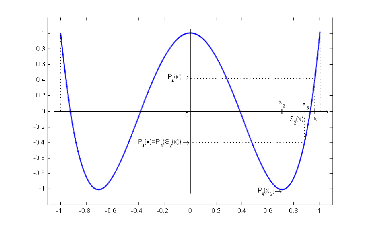
S_{n}:\left[x_{n+1},1\right]\rightarrow\left[x_{n},x_{n+1}\right].

the one-to-one mapping, such that:

P_{2^{n}}\left(x\right)=-P_{2^{n}}\left(S_{n}(x)\right),\,\,\,x_{n+1}\leq x\leq 1.

We have:

S_{n}(x_{n+1})=x_{n+1},\quad S_{n}(1)=x_{n},\,\,\,n=1,2,\dots

Refer to caption — Figure 1. The mapping $S_{2}$

Example 3.7.

We have:

S_{1}(y)=-y,\quad\frac{dS_{1}(y)}{dy}=-1,\quad x_{2}<y<1,

S_{2}(y)=\sqrt{1-y^{2}},\quad\frac{dS_{2}(y)}{dy}=-\frac{y}{\sqrt{1-y^{2}}},\quad x_{3}<y<1,

S_{3}(y)=\frac{y+\sqrt{1-y^{2}}}{\sqrt{2}},\quad\frac{dS_{3}(y)}{dy}=-\frac{y-\sqrt{1-y^{2}}}{\sqrt{2(1-y^{2})}},\quad x_{4}<y<1.

Definition 3.8.

For an arbitrary integral number $0\leq n$ and a function $f(x)$ defined on the interval $x_{n}\leq x\leq 1,$ let us denote by $R_{n}(f)$ the function defined on the interval $x_{n+1}<y<1$ by:

R_{n}(f)(y)=\frac{f\left(S_{n}(y)\right)+f(y)}{2}.

Remark 3.9.

If the function $f$ is constant on the interval $[-1,1]$ then for an arbitrary $0\leq n$ we have:

R_{n}(f)(y)=f(y),\quad\text{on}\quad x_{n+1}<y<1.

Remark 3.10.

For any of the polynomials $P_{k}(x),\,\,\,k=0,1,2,\dots$ which we constructed, we have:

R_{0}(P_{k})(x)=P_{k}(x),\quad k=0(mod2),

and

R_{0}(P_{k})(x)=0,\quad k=1(mod2).

Remark 3.11.

For any of the polynomials $P_{2^{p}k}(x),\,\,\,k,p=1,2,\dots$ , which we constructed, we have:

R_{p}(P_{2^{p}k})(x)=P_{2^{p}k}(x),\quad k=0(mod2),

and

R_{p}(P_{2^{p}k})(x)=0,\quad k=1(mod2).

Definition 3.12.

For natural $n$ we’ll denote by ${\bf W}_{n}$ the family of nonnegative functions $\rho(x),\,\,\,-1<x<1$ satisfying the following conditions:

\int_{-1}^{1}\rho(x)dx=1

and

\rho(y)=-\rho(S_{k}(y))\frac{dS_{k}(y)}{dy},\,\,x_{k}<y\leq 1,

for $k=0,1,2,\dots,n-1$ .

Remark 3.13.

Let us note that for an arbitrary weight function $\rho(x)\in{\bf W}_{n}$ we have:

(3.14)

\int_{x_{n}}^{1}\rho(y)dy=2^{-n}.

Moreover, an arbitrary nonnegative function defined on $[x_{n},\,1]$ satisfying the condition (3.14), coincides with a weight function from ${\bf W}_{n}$ on $[x_{n},\,1]$ .

Example 3.15.

Note, that:

S_{0}(y)=-y,\quad x_{1}\leq y\leq 1,

therefore for the weight function $\rho\in{\bf W}_{1}$ we get the condition:

\rho(y)=\rho(-y),\,\,x_{0}<y\leq 1.

Example 3.16.

We have:

S_{1}(y)=\sqrt{1-y^{2}},\quad x_{2}\leq y\leq 1,

therefore for the weight function $\rho\in{\bf W}_{2}$ we get the conditions:

\rho(y)=\rho(-y),\,\,x_{0}=-1<y\leq 1,

and

\rho(y)=\rho\left(\sqrt{1-y^{2}}\right)\frac{y}{\sqrt{1-y^{2}}},\,\,x_{1}<y\leq 1,

In particular, the function:

\rho(y)=\frac{1}{\pi\sqrt{1-y^{2}}}

satisfies these conditions.

Example 3.17.

We have:

S_{2}(y)=\frac{y+\sqrt{1-y^{2}}}{\sqrt{2}},\quad x_{3}\leq y\leq 1,

therefore for the weight function $\rho\in{\bf W}_{3}$ we get the conditions:

\rho(y)=\rho(-y),\,\,x_{0}<y\leq 1,

and

\rho(y)=\rho\left(\sqrt{1-y^{2}}\right)\frac{y}{\sqrt{1-y^{2}}},\,\,x_{1}<y\leq 1,

and

\rho(y)=\rho\left(\frac{y+\sqrt{1-y^{2}}}{\sqrt{2}}\right)\frac{y-\sqrt{1-y^{2}}}{\sqrt{2(1-y^{2})}},\quad x_{2}<y<1.

In particular, the following function:

\rho(y)=\frac{1}{\pi\sqrt{1-y^{2}}}

satisfies all the three conditions.

Remark 3.18.

By a reasoning similar to (3.16) and (3.17) one can prove that:

\rho(y)=\frac{1}{\pi\sqrt{1-y^{2}}}\in{\bf W}_{n}\;\text{for}\;n=1,2,\dots.

Remark 3.19.

The class ${\bf W}_{n}$ coincides with the family of non-negative functions $\rho(x)$ whose integral is equal to $1$ and who permit the following representation:

\rho(x)=\frac{w(x)}{\sqrt{1-x^{2}}},

where $w(x)$ satisfies the conditions:

w(x)=w(S_{k}(x)),\quad\text{for all}~k=0,1,\dots,n-1,~\text{and}~x_{k+1}<x\leq 1.

4. Main Results

Theorem 4.1.

Let $n\geq 1$ be a natural number. Let $\rho(x)\in{\bf W}_{n}$ . Then for an arbitrary function $f(x)$ we have:

\int_{-1}^{1}f(x)\rho(x)dx=2^{n}\int_{x_{n}}^{1}(R_{n-1}\circ\dots\circ R_{0})(f)(x)\cdot\rho(x)dx.

Proof.

If $\rho(x)\in{\bf W}_{1}$ we have $\rho(y)=\rho(-y)$ so,

\int_{-1}^{1}f(x)\rho(x)dx=\int_{-1}^{0}f(x)\rho(x)dx+\int_{0}^{1}f(x)\rho(x)dx=

=\int_{0}^{1}f(x)\rho(x)dx-\int_{0}^{1}f\left(S_{0}(y)\right)\rho\left(S_{0}(y)\right)\frac{dS_{0}(y)}{dy}dy=

=\int_{0}^{1}(f(x)+f(-x))\rho(x)dx=2\int_{x_{1}}^{1}R_{0}(f)(y)\rho(y)dy.

If $\rho(x)\in{\bf W}_{2}$ then we have $\rho(y)=\rho(-y)$ and

\rho(y)=-\rho\left(S_{1}(y)\right)\frac{dS_{1}(y)}{dy},\,\,x_{2}\leq y\leq 1.

Thus, for an arbitrary function $f(x)$ we have:

\int_{-1}^{1}f(x)\rho(x)dx=2\int_{x_{1}}^{1}R_{0}(f)(x)\rho(x)dx=2\int_{x_{1}}^{x_{2}}R_{0}(f)(x)\rho(x)dx+2\int_{x_{2}}^{1}R_{0}(f)(x)\rho(x)dx=

=2\int_{x_{2}}^{1}R_{0}(f)(x)\rho(x)dx-2\int_{x_{2}}^{1}R_{0}(f)\left(S_{1}(y)\right)\rho\left(S_{1}(y)\right)\frac{dS_{1}(y)}{dy}dy=

=2\int_{x_{2}}^{1}\left(R_{0}(f)\left(S_{1}(y)\right)+R_{0}(f)(y)\right)\rho(y)dy=2^{2}\int_{x_{2}}^{1}(R_{1}\circ R_{0})(f)(y)\rho(y)dy.

We prove the theorem for the other values of $n$ in an analogous way. ∎

Theorem 4.2.

Let $\rho(x)\in{\bf W}_{n}$ . Let $X=\{{t_{j}\}}_{j=1}^{m}$ be a certain set of points, for whom:

-1<t_{1}<t_{2}<\dots<t_{m}<1.

Let $X\cap\left[x_{n},1\right]\neq\emptyset$ and

S_{k}\left(X\cap\left[x_{k+1},1\right]\right)=X\cap\left[x_{k},x_{k+1}\right],\quad\text{for all}\quad k=0,1,2,\dots,n-1.

Then for an arbitrary polynomial $P(x)\in Pol(2^{n}-1)$ we have:

\int_{-1}^{1}P(x)\rho(x)dx=\frac{1}{m}\sum_{k=1}^{m}P(t_{k}).

Proof.

Remark (3.11) implies that:

\left(R_{n-1}\circ\dots\circ R_{0}\right)P_{k}=0,\quad\text{for}\quad k=1,\dots,2^{n}-1.

So, for each polynomial $P(x)\in Pol\left(2^{n}-1\right)$ we have $\left(R_{n-1}\circ\dots\circ R_{0}\right)P=const$ .

Thus, by theorem (4.1) we have:

\int_{-1}^{1}P(x)\rho(x)dx=(R_{n-1}\circ\dots\circ R_{0})(P)(t)\cdot 2^{n}\int_{x_{n}}^{1}\rho(x)dx,

for any $x_{n}\leq t<1$ . Further, by (3.13) we get:

\int_{-1}^{1}P(x)\rho(x)dx=(R_{n-1}\circ\dots\circ R_{0})(P)(t),

for any $x_{n}\leq t<1$ . This is why,

\int_{-1}^{1}P(x)\rho(x)dx=\frac{1}{|X\cap\left[x_{n},1\right]|}\sum_{x_{n}\leq t_{j}<1}(R_{n-1}\circ\dots\circ R_{0})(P)(t_{j}).

At this moment let’s consider the particular case $n=1$ . From (3.8) we have:

\frac{1}{|X\cap\left[0,1\right]|}\sum_{0\leq t_{j}<1}R_{0}(P)(t_{j})=\frac{1}{2|X\cap\left[0,1\right]|}\sum_{0\leq t_{j}<1}\left(P(t_{j})+P(-t_{j})\right)=\frac{1}{m}\sum_{k=1}^{m}P(t_{k}).

For the other values of $n$ the equality:

\frac{1}{|X\cap\left[x_{n},1\right]|}\sum_{x_{n}\leq t_{j}<1}(R_{n-1}\circ\dots\circ R_{0})(P)(t_{j})=\frac{1}{m}\sum_{k=1}^{m}P(t_{k}).

is proved in an analogous way.

∎

Remark 4.3.

Theorem (4.2) implies that for any $\rho\in\bf W_{n}$ we have:

m=|X|\geq 2^{n-1}.

If we additionally impose that:

t_{m}=x_{n},

then we get that $|X|=m=2^{n-1}$ and the quadrature formula is valid for an arbitrary poynomial $P(x)\in Pol\left(2^{n}-1\right)$ . Hence,

M_{2^{n-1}}(\rho)\geq 2^{n}-1

M_{m}(\rho)\geq 2m-1,\quad\text{for}\quad m=2^{n-1}.

But taking into account the remark (1.6), we get that:

M_{m}(\rho)=2m-1,\quad\text{for}\quad m=2^{n-1}.

Remark 4.4.

Remark (4.3) shows that we found a Chebyshev - type quadrature formula for $\rho\in\bf W_{n}$ of the highest possible degree $2^{n}-1$ , where the number of nodes is $m=2^{n-1}$ .

References

[1] J. Korevaar and J.L.H. Meyers, Spherical Faraday cage for the case of equal point charges and Chebyshev-type quadrature on the sphere, Integral Transform. Spec. Funct. 1 (1993), no. 2, 105–117.
[2] J. Korevaar and M.A. Monterie, Approximation of the equilibrium distribution by distributions of equal point charges with minimal energy, Trans. Amer. Math. Soc. 350 (1998), no. 6, 2329–2348.
[3] A. Kuijlaars, The minimal number of nodes in Chebyshev type quadrature formulas, Indag. Math. (N.S.) 4 (1993), no. 3, 339–362.
[4] A. B. J. Kuijlaars, Chebyshev quadrature for measures with a strong singularity, Proceedings of the International Conference on Orthogonality, Moment Problems and Continued Fractions (Delft, 1994), J. Comput. Appl. Math. 65 (1995), no. 1-3, 207-214.
[5] J.L. Ullman, A class of weight functions that admit Tchebycheff quadrature, Michigan Math. J. 13 (1966), 417–423.
[6] K.-J. Förster, Variace in quadrature - a survey, Numerical Integration 4 (Birkhauser, Basel) (1993), pp 91-110.
[7] E. B. Saff and A. B. J. Kuijlaars, Distributing many points on a sphere, Math. Intelligencer 19 (1997), no. 1, 5-11.
[8] S.N. Bernstein, On quadrature formulas with positive coefficients (in Russian), Izv. Akad. Nauk SSSR Ser. Mat. 4 (1937), 479-503.
[9] S.N. Bernstein, Sur la formule de quadrature approche de Tchebycheff , Comptes Rendus 203 (1936), 1305-1306.
[10] V. I. Krilov, Priblizhennoe vychislenie integralov (in Russian), Moscow, (1959).
[11] K.A. Posse, Sur les quadratures, Nouv. Ann. de Math. 26 (1875), 49-62.

Chebyshev-Type Quadrature Formulas for New Weight Classes

Abstract.

1. Introduction

Definition 1.1.

Remark 1.3.

Remark 1.5.

Proof.

Remark 1.6.

Theorem 1.7 (Mehler).

Theorem 1.8.

2. The Case ρ≡1/2\rho\equiv 1/2

Theorem 2.1.

3. Auxiliary Constructions

Definition 3.1.

Example 3.2.

Theorem 3.3.

Proof.

Example 3.4.

Theorem 3.5.

Definition 3.6.

Example 3.7.

Definition 3.8.

Remark 3.9.

Remark 3.10.

Remark 3.11.

Definition 3.12.

Remark 3.13.

Example 3.15.

Example 3.16.

Example 3.17.

Remark 3.18.

Remark 3.19.

4. Main Results

Theorem 4.1.

Proof.

Theorem 4.2.

Proof.

Remark 4.3.

Remark 4.4.

References

2. The Case $\rho\equiv 1/2$