From hardcore Bosons to free Fermions with Painlevé V

Denoting an eigenfunction of the Hamiltonian (1) by $\Psi(x_{1},\ldots,x_{N},y)$, we require it to be antisymmetric in the first $N$ arguments. This and the fact that there is no interaction between the particles of the Fermi-sea suggest to write $\Psi(x_{1},\ldots,x_{N},y)$ as a determinant

Note that $\Psi(x_{1},\ldots,x_{N},y)$ has all required symmetries i.e. is antisymmetric under the exchange of all quasimomenta, antisymmetric in the particle postions $x_{l}$ , $l=,1,\ldots,N$ and has no well defined symmetry when the distinguishable particle and a particle of the Fermi–sea are exchanged. As shown in Sec. 3.2 the normalization constant $C_{N}$ is for periodic boundary conditions determined by (see Eq. (75))

In Eq. (2) $\{k_{j}\}_{j=1,\ldots,N+1}$ are the ”quasimomenta” and $\Lambda$ is an additional parameter (not present in [14, 15]).

The wave function (2) is an eigenfunction of the Hamiltonian (1) to the eigenvalue

Furthermore the eigenvalue to the center of mass momentum operator is

The form (2) is crucial for our approach, since it allows us to employ powerful methods of matrix algebra to manipulate determinants. Equations (2)-(5) can be proved straightforwardly by acting with $\hat{H}$ on $\Psi$.

In order to acquire results for finite particle density we impose periodic boundary conditions

The first condition yields the transcendental equations

which after taking the logarithm on both sides translates to

As can be seen by considering the limit $c\to 0$ of Eq. (9) the numbers $n_{j}$ have to be half-integers and $-\pi/2$ $<\arctan(x)$ $<\pi/2$. The second condition (7) yields

where $\tilde{n}_{j}$ are half-integers for $N$ odd and integers for $N$ even. In the following we will for convenience always assume $N$ to be odd.

Combining Eq. (8) and Eq. (10) yields quantization rules for the quasimomenta $k_{j}$ and $\Lambda$ which are known as Bethe–Ansatz equations

Now the $m_{j}$ are unequal integers. According to Eq. (12) the integer $J_{\Lambda}$ is bounded by

The quantities $m_{j},J_{\Lambda}$ are the quantum numbers labeling an eigenstate of the system. For $J_{\Lambda}=\Lambda$ $=0$ an expression equivalent to Eq. (11) was derived in Ref. [14]. For a derivation of Eqs. (11) and (12) from the Bethe–Ansatz wave function we refer to Ref. [7].

The Bethe-Ansatz equations are coupled algebraic equations which in general do not permit a closed solution. In our case the situation is more favorable, since the equations for $k_{j}$ only couple via $\Lambda$. For $c\to 0$ and for $c\to$ $\infty$ they can be solved exactly.

Let $\{m_{j}\}_{j=1,\ldots,N+1}$ be a set of ordered integers $m_{j}>m_{j+1}$. Then in the limit $c\to 0^{+}$ a solution to the Bethe–Ansatz equations (11) and (12) is given by

and $\Lambda\in[m_{j},m_{j+1}+1]$. The superscript $\pm$ indicates that $k_{j}$ is approaching its value from above/below. For $c\to 0^{+}$ the solution for $\Lambda$ is in general not unique. We come back to this point below.

Since the quantum numbers $m_{j}$ and $J_{\Lambda}$ for the ground state are the same for $c=0$ and $c>0$, the quantum numbers $m_{j}$ of the interacting ground state can be extracted from Eq. (2.2)

This yields for $c=0$ the set of quasimomenta

Since the distinguishable particle can occupy the same state as a sea-particle, in the ground state the single particle quasimomentum with the lowest energy is double occupied. Thus for the ground state $J_{\Lambda}=0$. The allowed interval for $\Lambda$ shrinks to a point and the solution for $\Lambda$ becomes unique $\Lambda=0$. The same happens for any other state for which $m_{J_{\Lambda+(N+1)/2}}$ and $m_{(J_{\Lambda+(N+1)/2}+1)}$ are adjacent integers.

In the hardcore limit $c\rightarrow\infty$ Eqs. (11) and (12) become

where the dimensionless factor $\lambda$ takes into account that $\Lambda$ scales like $c$ for $c\rightarrow\infty$. From the definition in Eq. (20) it is seen that $\lambda$ can range between $-\infty$ and $\infty$ when $J_{\Lambda}$ varies according to Eq. (13).

For finite $c$ the Bethe–Ansatz equations can be calculated numerically. As $c$ increases the quasimomenta $k_{j}$ evolve smoothly from $2\pi(m_{j}+\theta(\Lambda-m_{j}))/L$ to $2\pi(m_{j}+{\scriptstyle\frac{1}{2}}\textrm{sgn}(\Lambda-m_{j}))L$, i. e. from multiple integer to multiple half–integer values of $2\pi/L$. The additional parameter $\Lambda$ evolves smoothly from its initial value to $\pm\infty$ as the interaction increases.

In the following we assume that the sea–particles are in the ground state but the extra particle may occupy an arbitrary single particle state. Two cases have to be distinguished:

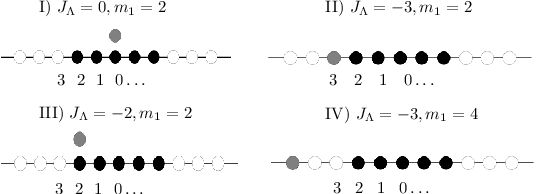
Either the quasimomentum of the extra particle lies inside the Fermi–sea. Then the quantum numbers $m_{j}$ of the state are given by the set of integers in Eq. (17). The non–interacting extra particle shares its momentum with one of the particles of the Fermi–sea. The additional quantum number $J_{\Lambda}$ indicates the double occupied quasimomentum. For $J_{\Lambda}=(N-1)/2$ or $J_{\Lambda}$ $=-(N-1)/2$ the Fermi–momentum of the sea is double occupied. The non–interacting eigenfunctions for a given set of quasimomenta $\{k_{j}\}_{j=1,\ldots,N+1}$ is uniquely determined and the energy–eigenvalue is non–degenerate. Thus for $c=0$ the energy increases quadratically with $J_{\Lambda}$.

In the second case the quasimomentum of the extra particle lies outside the Fermi–sea. The quantum number $J_{\Lambda}$ takes its value at the upper edge $J_{\Lambda}=(N+1)/2$ or at the lower edge $J_{\Lambda}=-(N+1)/2$ of its spectrum. For vanishing interaction all $N+1$ quasimomenta are different. If the highest/lowest quantum number is $m_{1}=(N-1)/2$ respectively $m_{N+1}=-(N+1)/2$ the extra particle’s momentum borders the Fermi–sea. If $m_{1}>(N-1)/2$ or $m_{N+1}<-(N+1)/2$ the extra particle’s momentum is outside the Fermi sea. For a given set of quasimomenta there exist $N+1$ orthogonal eigenfunctions since the extra particle might carry any of the $k_{n}$’s without changing the systems energy. These eigenfunctions are distinguished by $J_{\Lambda}$. Thus at the Fermi–edge the energy becomes independent of $J_{\Lambda}$ and the density of states has a singularity. The different cases are illustrated in Fig. 1.

Summation over Eq. (11) from $j=1$ to $j=N+1$ yields in combination with Eq. (12) for the overall momentum of the system

If the set $\{m_{j}\}_{j=1,\ldots,N+1}$ is given by Eq. (17) the sum vanishes and the quantum number $J_{\Lambda}=-\frac{LK}{2\pi}$ is directly related with the center of mass momentum $K$. The latter in turn is identified with the momentum of the extra particle in the lab frame where the Fermi–sea is at rest.

For a dense set of quantum numbers as in Eq. (17) the density of states $\varrho(k)=\partial m(k)/\partial k$ can be derived by taking the derivative of Eq. (11)

This expression has a rather natural interpretation: The first term corresponds to the density of states of a non-interacting Fermi–sea. The second term appears due to the presence of the distinguishable particle. It has the form of a Lorentzian distribution centered around $\Lambda$ with width $c$. For $c\rightarrow 0$ it becomes a $\delta$-function at $k=\Lambda$.

In the thermodynamic limit, where $N,L\rightarrow\infty$ such that the particle density $\rho=N/L$ remains finite there are different choices for the scaling of the interaction strength

The Lorentzian part in Eq. (22) is outscaled by the part due to the Fermi-sea in all three cases. This implies that in the thermodynamic limit the single particle does not affect the spectrum of the Fermi-sea. The effect of the particle onto the bath should therefore be negligible. This is of course an essential requirement for a bona fide dissipative quantum system.

The system’s total energy is

For the energy shift due to the interaction this yields up to corrections of order $1/N$

where the Fermi-momentum is $k_{\rm F}=\pi\rho+{\cal O}(N^{0})$ and

corresponds to the energy of the non–interacting system. In the thermodynamic limit where the quasimomenta are distributed according to Eq. (17), it proves useful to define the quantity $\hat{K}=K/k_{\rm{F}}=2J_{\Lambda}/N$. It corresponds to the overall momentum in units of $k_{\rm F}$ and measures the position, where the extra particle’s momentum is located in the Fermi–sea . For $\hat{K}=0$ the extra particle’s momentum is in the center, for $\hat{K}=\pm 1$ it is at the upper or lower edge.

Since it appears frequently troughout the following we introduced in Eq. (25) the abbreviation

Note that the parameter $\Lambda$ in Eq. (25) is not independent but relates via the second Bethe-Ansatz equation (12) to $J_{\Lambda}$, $k_{\rm F}$ and $c$

From this equation follows in particular that $\Lambda|_{c=0}=-2\pi J_{\Lambda}/L$.

Although the integral can be evaluated the resulting transcendental equation can not be solved analytically for $\Lambda$. Therefore the energy shift can in general not be expressed as function of the three independent quantities $J_{\Lambda}$, $k_{\rm F}$ and $c$ and has to be calculated numerically. For the ground state where $J_{\Lambda}=\Lambda=0$, the situation is more favorable and the expression (25) simplifies to

The mean interaction energy

can be obtained using Pauli’s trick (see Ref. [29]) as

The interaction energy is given by the interaction strength times the probability to find a sea-particle at the same position as the extra particle. The latter is identical with the equal time density–density correlation function $R(x,y)$ at $x=y=0$. Thus we have, by definition,

Equating Eqs. (31) and (32) yields

Thus the probability to find a sea particle at the position of the extra particle vanishes as $c^{-2}$ for $c\to\infty$. Therefore the interaction energy vanishes in the weak coupling limit as well as in the strong coupling limit.

In Sec. 4, where the full density–density correlation function is studied, we derive an expression for $R(0,0)$ for $J_{\Lambda}\neq 0$, see Eq. (92). This allows us to calculate the interaction energy in this case as well. In Fig.  2 the ground state energy shift and interaction energy are plotted versus the interaction strength for three different values of $\hat{K}$.

It is seen that the interaction energy has a maximum as predicted. The ground state energy shift increases monotonously and saturates at a value $E_{\rm max}=$ $k_{\rm F}^{2}-K^{2}$. This means that for the extra particles momentum located right at the edge of the Fermi–sea the energy shift vanishes for arbitrary interaction strength.

Using the wave function (2) the mean expectation value of the extra particles energy can be calculated. Up to corrections of order $1/N$ we obtain

For the ground state this simplifies to

From Eq. (35) it is seen that the extra particles energy increases monotonically from $\langle\hat{p}_{y}^{2}\rangle=0$ to $\langle\hat{p}_{y}^{2}\rangle=k_{\rm F}^{2}/3$ as $\hat{c}$ varies from zero to $+\infty$.

For $c\rightarrow\infty$ the wave function (2) becomes

where we recall $\lambda=\Lambda/c$. For $\lambda=0$ the expression resembles the wave function of $N+1$ hardcore Bosons [6]. The only difference consists in the product of sign–functions: The wave function for hardcore Bosons is a Slater determinant multiplied not with a single product of sign-functions but with a double product $\prod_{i<j}\textrm{sgn}(x_{i}-x_{j})$. For the equal time Green’s function this difference is irrelevant and it is identical with those of hardcore Bosons. A large body of literature has been devoted to the studies of the latter [30, 24, 31, 32, 26, 27, 28, 33, 34, 35].

On the other hand for $|\lambda|\rightarrow\infty$ the wave function and therefore also the Green’s function coincides with that of free Fermions. This is already reflected in the Bethe-Ansatz equations (19) and (20). The quasimomenta are integer multiples of $2\pi/L$ with an offset $\arctan(\lambda)/\pi$ which ranges from zero to $\pm{\scriptstyle\frac{1}{2}}$ for $|\lambda|\rightarrow\infty$.

Hence varying $\lambda$ from $\lambda=0$ to $\lambda=\infty$ we expect the extra particle to undergo a transition from a hardcore Boson to a free Fermion. This transition should be reflected in the equal time Green’s function. As there are two fundamental formulations of the Green’s function for impenetrable Bosons we will go for two different ways to study it. The first approach is based on the theory of Töplitz determinants [30, 24, 25, 27] and will be reviewed in the appendix A.

The second approach is the description of the Green’s function via solutions of a Painlevé equation [26, 28]. In the following we are going to show that the above mentioned transition is for zero temperature described by a change in the initial condition of the solution of one and the same Painlevé equation.

We plug Eq. (45) into the definition (36) of the equal time Green’s function. This yields

The crucial point is that for zero temperature, or – more precisely – if the Fermi–sea is in the ground state, the integral can be interpreted as an average over the unitary group. We rewrite the last line of the equation above according to

In the present case the first product can be identified with the measure of the unitary group $U(N)$ [36]

The Green’s function can again be written like in Eq. (42), where the part $G_{\rm{I}}$, which includes the effects of interaction, is identified with the average of the function

with respect to the measure $d\mu(U)$. Here we have introduced the indicator function

and the parameter

Averages over the unitary group of functions of the type (49) were studied by Forrester, Frankel, Garoni and Witte [37, 27, 28] and they have been related to solutions of the Painlevé VI non–linear differential equation. Defining

we follow Proposition 3 and Corollary 1 of Ref. [28] in order to deduce the relation

for the interaction part of the Green’s function. The function $\sigma_{N}(u)$ is a solution of the particular $P_{\rm{VI{}}}$ $\sigma$-form due to Okamato [38]

The initial conditions are fixed by expanding $G_{\rm I}(y^{-})$ for small distances like in Ref. [28]. We find that in terms of the variable $u$ the solution of Eq. (54), quested for, has the small distance expansion

In the thermodynamic limit the expressions simplify further. First, Painlevé VI converts in the limit $N\to\infty$ to the Jimbo–Miwa–Okamoto form [26, 39] of the Painlevé V differential equation

where $x=k_{\rm F}y^{-}$. Second, the initial condition for $\sigma_{{V{}}}(x)$ becomes

Thus the Green’s function reads in the thermodynamic limit

The long distance behavior of $G_{\rm{I}}(x)$ can be related to the short distance behavior (57), i. e. to $\lambda$ with a connection formula for Painlevé equations. The case of Painlevé V has been solved by McCoy and Tang [40, 41, 42]. We employ the results obtained in Ref. [41] for hardcore Bosons:

Let the solution of Painlevé V in the Jimbo-Miwa-Okamoto sigma form as given in Eq. (56) be regular at $x=0$ with the expansion

Then for general $\xi\in{\mathbb{C}}$ the asymptotic expansion for $x\to\infty$ is different for $\xi\in(1,\infty)$ (case I) and for $\xi\in{\mathbb{C}}\setminus(1,\infty)$ (case II). In the first case it its given by

where the parameters $k_{\rm I},\phi_{\rm I}$ depend on $\xi$ as

References

- (1) T. Gianmarchi. Quantum Physics in one dimension. Oxford University Press, Oxford, 2004.
- (2) A. Imambekov, T. L. Schmidt, and L. I. Glazman. One-Dimensional Quantum Liquids: Beyond the Luttinger Liquid Paradigm. arXiv:1110.1374, 2011.
- (3) F. D. M. Haldane. Luttinger Liquid theory of one–dimensional quantum fluids. J. Phys. C, 14:2585, 1981.
- (4) G. Barak, H. Steinberg, Loren N. Pfeiffer, Ken W. West, L. Glazman, F. von Oppen, and A. Yacoby. Interacting electrons in one dimension beyond the Luttinger-liquid limit. Nature Physics, 6:489, 2010.
- (5) T. Kinoshita, T. Wenger, and David S. Weiss. A quantum Newton’s cradle. Nature Letters, 900:1005, 2006.
- (6) E. Lieb and W. Liniger. Exact Analysis of an Interacting Bose Gas. I. The General Solution and the Ground State. Phys. Rev., 130:1605, 1963.
- (7) M. Takahashi. Thermodynamics of One–dimensional Solvable Models. Cambridge University Press, Cambridge, 1999.
- (8) M.A. Cazalilla. Bosonizing one-dimensional cold atomic gases. J. Phys. B, 37:1, 2004.
- (9) C. N. Yang. Some Exact Results for the Many-Body Problem in one Dimension with Repulsive Delta-Function Interaction. Phys. Rev. Lett., 19:1312, 1967.
- (10) Gaudin. Un systeme a une dimension de Fermions en interaction. Phys. Lett., 24A:55, 1966.
- (11) V. E. Korepin, N. M. Bogoliubov, and A. G. Izergin. Quantum Inverse Scattering Method and Correlation Functions. Cambridge University Press, Cambridge, 1st edition, 1993.
- (12) V. V. Cheianov and M. B. Zvonarev. Zero temperature correlation functions for the impenetrable fermion gas. Phys. Rev. A, 37:2261, 2004.
- (13) A. Imabekov and E. Demler. Exactly solvable case of a one-dimensional Bose˘Fermi mixture. Phys. Rev. A, 73:021602, 2006.
- (14) J. B. McGuire. Interacting Fermions in One Dimension. I. Repulsive Potential. J. Math. Phys., 6:432, 1965.
- (15) J. B. McGuire. Interacting Fermions in One Dimension. II. Attractive Potential. J. Math. Phys., 7:123, 1966.
- (16) C.K. Lai and C.N. Yang. Ground-State Energy of a Mixture of Fermions and Bosons in One Dimension with a Repulsive -Function Interaction. Phys. Rev. A, 3:393, 1971.
- (17) A. Imabekov and E. Demler. Ann. Phys., 321:2390, 2006.
- (18) K. B. Gubbels and H. T. C. Stoof. Renormalization Group Theory for the Imbalanced Fermi Gas. Phys. Rev. Lett., 100:140407, 2008.
- (19) Z.-J. Ying, M. Cuoco, C. Noce, and H.-Q. Zhou. Exact Solution for a trapped Fermi Gas with Population Imbalance and BCS Pairing. Phys. Rev. Lett., 100:140406, 2008.
- (20) M. Klaus. Bose Condensates and Fermi Gases at Zero Temperature. Phys. Rev. Lett., 80:1804, 1998.
- (21) A. G. Truscott, K.E. Strecker, W.I. McAlexander, G.B. Partridge, and R.G. Hulet. Observation of Fermi Pressure in a Gas of Trapped Atoms. Science, 291:2570, 2001.
- (22) K. Pilch et al. Observation of interspecies Feshbach resonances in an ultracold Rb-Cs mixture. Phys. Rev. A, 79:042718, 2009.
- (23) M.L. Olsen, J.D. Perreault, T.D. Cumby, and D.S. Jin. Coherent atom-molecule oscillations in a Bose-Fermi mixture. Phys. Rev. A, 80:030701, 2009.
- (24) A. Lenard. Some remarks on large Toeplitz determinants. Pacific J. Math, 42:137, 1972.
- (25) H. Widom. Toeplitz determinants with singular generating functions. Am. J. Math., 95:333, 1973.
- (26) M. Jimbo, T. Miwa, Y. Mori, and M. Sato. Density matrix of an impenetrable Bose gas and the fifth Painleve transcendent . Phys. D, 1:80, 1980.
- (27) P. J. Forrester, N. E. Frankel, T. M. Garoni, and N. S. Witte. Finite one-dimensional impenetrable Bose systems: Occupation numbers. Phys. Rev. A, 67:043607, 2003.
- (28) P. J. Forrester, N.E. Frankel, T.M. Garoni, and N.S. Witte. Painleve transcendent evaluations of finite systems density matrices for 1d impenetrable Bosons. Communications in Mathematical Physics, 238:257–285, 2003.
- (29) A.L. Fetter and J.D. Walecka. Quantum theory of many particle systems. McGraw-Hill, New York, 1971.
- (30) A. Lenard. Momentum Distribution in the Ground State of the One-Dimensional System of Impenetrable Bosons. J. Math. Phys., 5:930, 1964.
- (31) H. G. Vaidya and C. A. Tracy. One particle reduced density matrix of impenetrable bosons in one dimension at zero temperature. J. Math. Phys., 20:2291, 1979.
- (32) H.G. Vaidya and C.A. Tracy. One particle reduced density matrix of impenetrable bosons in one dimension at zero temperature. Phys. Rev. Lett., 42:3, 1979.
- (33) P.J. Forrester, N.E. Frankel, and T.M. Garoni. Random matrix averages and the impenetrable Bose gas in Dirichlet and Neumann boundary conditions. J. Math. Phys, 44:4157, 2003.
- (34) P.J. Forrester, N.E. Frankel, and I.M. Makin. Analytic solutions of the one-dimensional finite-coupling delta-function Bose gas. Phys. Rev. A, 74:043614, 2006.
- (35) T. Papenprock. Ground-state properties of hard-core bosons in one-dimensional harmonic traps. Phys. Rev. A, 67:41601, 2003.
- (36) M.L. Metha. Random Matrices. Academic Press Inc., New York, 2004.
- (37) P. J. Forrester and N. S. Witte. Application of the -Function Theory of Painlevé Equations to Random Matrices: PIV, PII and the GUE. Comm. Math. Phys., 219:357, 2001.
- (38) K. Okamato. Studies on the Painlevé equations I.-Sixth Painlevé equation PVI. Annali di Matematica Pura ed Applicata, 146:337, 1986.
- (39) Okamoto K. Studies on the Painlevé equations. II. Fifth Painlevé equation . Japan. J. Math. (N.S.), 13(1):7, (1987).
- (40) B.M. McCoy and S. Tang. Connection formulae for Painlevé V functions. Physica D, 19:42–72, 1986.
- (41) B.M. McCoy and S. Tang. Connection formulae for Painlevé V functions II, the function Bose gas problem. Physica D, 20:187–216, 1986.
- (42) B.M. McCoy and S. Tang. Connection formulae for Painlevé functions. Physica D, 18:190–6, 1986.
- (43) D. M. Gangardt and G. Shlyapnikov. Local correlations in a strongly interacting one-dimensional Bose gas. New Jour. Phys., 5:79, 2003.
- (44) Dennis B. Creamer, H.B. Thacker, and D. Wilkinson. Some exact results for the two point function of an integrable quantum field theory. Phys. Rev. D, 23:3081, 1981.