Dynamical (super)symmetry vacuum properties of the supersymmetric Chern-Simons-matter model

One of the main reasons for incorporating supersymmetry (susy) in realistic quantum field theories (the standard model of particle physics) is that this solves the gauge hierarchy problem, stabilizing the Higgs mass against quadratic radiative corrections. However, since supersymmetry has not been observed in Nature so far, it must be realized only in its broken form. In this context dynamical supersymmetry breaking (DSB), a beautiful phenomenon that occurs when the supersymmetry of the vacuum at tree-level is broken by dynamical (perturbative or non-perturbative) effects, has a privileged place in today’s physics. Indeed, DSB not only explains the stability of the Higgs boson, but also the origin of the small mass ratios in the theory [1]. In four dimensions (4D) DSB by perturbative effects (also known as Coleman-Weinberg’s mechanism) is forbidden by nonrenormalization theorems [2]. These theorems state that if supersymmetry is unbroken at tree level, then it remains so to all orders in perturbation theory. DSB therefore can only occur in 4D by nonperturbative effects (instantons, for example).

The nonexistence of such theorems in three dimensions (3D), in contrast, opens the door for investigating this phenomenon owing to radiative corrections in 3D supersymmetric field theories. In this paper, in particular, we study the dynamical (super)symmetry properties of the vacuum of the three dimensional $\mathcal{N}=1$ susy Chern-Simons model minimally coupled to a massless self interacting matter field (SCSM₃).

Our interest in this kind of models is motivated in part by their involvement in the construction of more complicated theories such as the Bagger-Lambert-Gustavsson (BLG) theory [3] and the Aharony-Bergman-Jafferis-Maldacena (ABJM) theory [4] in connection with the AdS₄/CFT₃ correspondence. In fact, in [5] and [6] it was shown that the BLG/ABJM theory in terms of 3D $\mathcal{N}=1$ superfields [7] involves two non-Abelian supersymmetric Chern-Simons fields with opposite signs and matter fields in the fundamental representation of the groups, coupled to the two Chern-Simons fields (bifundamental matter). Moreover, 3D gauge Chern-Simons theories are important in their own right, as they exhibit some remarkable features such as their topological nature [8] (quantization of the Chern-Simons coupling constant) and their link with three dimensions through the $\epsilon_{\mu\nu\rho}$-tensor. As far as physical applications are concerned, they play a significant role in condensed-matter phenomena, e. g., in quantum Hall effect [9] and high-T_c superconductivity [10].

In this paper the behavior of the vacuum in SCSM₃ under radiative corrections has been investigated by analyzing the minimum (or minima) of the effective potential computed up to two loops in the superfield perturbative formalism. The one-loop correction to the effective potential was calculated by the tadpole method [11], while the two-loop correction was calculated by the vacuum bubble method [12]. Since in both methods the scalar superfields must be shifted by their $\theta$ dependent vacuum expectation values, we have to face the difficulty of dealing with an explicit breakdown of supersymmetry in the intermediate stages of the calculation. Fortunately, the projection operator method developed in [13] and recently extended in [14] allows us to derive the supergraph Feynman rules, in particular, the superpropagators for the broken susy theory. With this method, each superpropagator of the shifted theory is expressed in terms of a basis of operators in the respective sector.

The paper is structured as follows. In Sec. II the three-dimensional $\mathcal{N}=1$ supersymmetric Chern-Simons model coupled to matter is introduced in the superfield formalism and its corresponding shifted theory is constructed. The superpropagators of the shifted theory are derived via the projection operator method. In Sec. III the evaluation of the effective potential (in the Landau gauge $\alpha\rightarrow 0$ and $\sigma_{2}$-linear approximation) is carried out by means of the tadpole method and the vacuum bubble method. As argued in the body of the paper these approximations are sufficient for our purposes. The Appendices contain some details of the calculations.

In the $D=3$ $\mathcal{N}=1$ superfield formalism, the building blocks of supersymmetric Abelian gauge theories are (1) a complex scalar (matter) superfield $\Phi\left(x,\,\theta\right)$ and (2) a spinor gauge potential $A_{\alpha}\left(x,\,\theta\right)$. Adopting the notation of [15], the component-field contents of these superfields are given by

$$\Phi(x,\,\theta)=\varphi\left(x\right)+\theta^{\alpha}\psi_{\alpha}\left(x\right)-\theta^{2}F\left(x\right)$$

(1)

and

$$A_{\alpha}\left(x,\,\theta\right)=\chi_{\alpha}\left(x\right)-\theta_{\alpha}B(x)+i\theta^{\beta}V_{\alpha\beta}\left(x\right)-\theta^{2}\left(2\lambda_{\alpha}+i\partial_{\alpha\beta}\chi^{\beta}\right).$$

(2)

Using these superfields along with the supersymmetric gauge covariant derivative $\nabla_{\alpha}\doteq D_{\alpha}-ieA_{\alpha}$, with $D_{\alpha}\doteq\partial_{\alpha}+i\theta^{\beta}\partial_{\alpha\beta}$, the three-dimensional $\mathcal{N}=1$ supersymmetric Chern-Simons model coupled to matter (SCSM₃) is described by the action

$$S=\int d^{5}z\left\{A^{\alpha}W_{\alpha}-\frac{1}{2}\overline{\nabla}^{\alpha}\overline{\Phi}\nabla_{\alpha}\Phi-g\left(\overline{\Phi}\Phi\right)^{2}\right\},$$

(3)

where $W_{\alpha}\doteq\frac{1}{2}D^{\beta}D_{\alpha}A_{\beta}$ is the superfield strength that satisfies the Bianchi identity $D^{\alpha}W_{\alpha}=0$.

The action (3) is invariant under the following infinitesimal gauge transformations

$$\Phi^{\prime}=\left(1+ieK\right)\Phi,\qquad A^{\prime}_{\alpha}=A_{\alpha}+D_{\alpha}K,$$

(4)

with $K\left(x,\,\theta\right)$ denoting an arbitrary real scalar superfield,

$$K\left(x,\,\theta\right)=\omega\left(x\right)+\theta^{\alpha}\sigma_{\alpha}\left(x\right)-\theta^{2}\tau\left(x\right).$$

(5)

Notice that under these transformations the superfield strength $W_{\alpha}$ is invariant $\left(W^{\prime}_{\alpha}=W_{\alpha}\right)$, whereas the derivative $\nabla_{\alpha}$ transforms like a covariant object, namely, $\nabla^{\prime}_{\alpha}\Phi^{\prime}=\left(1+ieK\right)\nabla_{\alpha}\Phi$.

Since our purpose is to calculate the two-loop effective potential by means of the tadpole method [11] at one-loop order and the vacuum bubble method [12] at two-loop order, we must appropriately choose the gauge fixing term in order to quantize the theory. The simplest choice compatible with both methods is the Lorentz-like gauge fixing term,

$\displaystyle S_{FG}$

$\displaystyle=$

$\displaystyle\int d^{5}z\,\left(-\frac{1}{4\alpha}\right)D^{\alpha}A_{\alpha}D^{\beta}A_{\beta},$

(6)

where $\alpha$ is a dimensionless parameter. The advantage of fixing the gauge in this way is that the Faddeev-Popov ghosts remain free and can be ignored.

Writing the complex matter superfield $\Phi$ in terms of two real superfields $\Sigma$ and $\Pi$,

$$\Phi=\frac{1}{\sqrt{2}}\left(\Sigma+i\Pi\right),$$

(7)

and adding (6) to (3), the classical action reads

	$\displaystyle S$	$\displaystyle=$	$\displaystyle\int d^{5}z\left\{\frac{1}{2}A_{\alpha}\left[-D^{\beta}D^{\alpha}-\frac{1}{2\alpha}D^{\alpha}D^{\beta}\right]A_{\beta}+\frac{1}{2}\Sigma D^{2}\Sigma+\frac{1}{2}\Pi D^{2}\Pi-\frac{e}{2}D^{\alpha}\Sigma A_{\alpha}\Pi\right.$		(8)
			$\displaystyle\left.+\frac{e}{2}D^{\alpha}\Pi A_{\alpha}\Sigma-\frac{e^{2}}{2}\left(\Sigma^{2}+\Pi^{2}\right)A^{2}-\frac{g}{4}\left(\Sigma^{2}+\Pi^{2}\right)^{2}\right\}.$

A simple dimensional analysis ($c=\hbar=1$) shows that all theory’s parameters, i.e. $\alpha$, $e$ and $g$ are dimensionless. Hence this model is a kind of 3D susy version of the conformally invariant Coleman-Weinberg model [16] (for this reason it is sometimes called, in the literature, the 3D susy Coleman-Weinberg model). Furthermore, it should be noted that the quadratic term in the gauge superfield $A_{\alpha}$ is not the Maxwell term, but instead the well-known Chern-Simons term

$$-\int d^{5}z\frac{1}{2}A_{\alpha}D^{\beta}D^{\alpha}A_{\beta}=-\int d^{3}x\frac{1}{2}\epsilon^{\mu\nu\rho}v_{\mu}\partial_{\nu}v_{\rho}+\cdots,$$

(9)

where the ellipsis represents other terms, $\epsilon^{\mu\nu\rho}$ $\left(\epsilon^{012}\doteq 1\right)$ is the completely antisymmetric tensor in the Minkowski space, and $v_{\mu}$ is the three vector given by $v_{\mu}\doteq\left(\gamma_{\mu}\right)^{\alpha\beta}V_{\alpha\beta}$.

In order to compute the effective potential by using the tadpole [11] and the vacuum bubble [12] methods, we must shift in (8) both scalar superfields ($\Sigma$, $\Pi$):

$$\Sigma\rightarrow\Sigma+\sigma\left(\theta\right),\qquad\Pi\rightarrow\Pi+\pi\left(\theta\right),$$

(10)

where $\sigma\left(\theta\right)\doteq\sigma_{1}-\theta^{2}\sigma_{2}$ and $\pi\left(\theta\right)\doteq\pi_{1}-\theta^{2}\pi_{2}$, with $\sigma_{i}$ and $\pi_{i}$ being $x$-constant classical fields ($\sigma_{1}$ and $\pi_{1}$are dynamical component fields and $\sigma_{2}$and $\pi_{2}$ are auxiliary fields, whose non-null values imply in breakdown of susy in the intermediate steps of the calculations). However, we can make use of the rotational $SO(2)$ symmetry, $\sigma^{\prime}_{i}+i\pi^{\prime}_{i}=\exp\left(i\,e\,\omega\right)\left(\sigma_{i}+i\pi_{i}\right)$, that the effective potential inherits from the classical action, to simplify the calculations. By taking advantage of this symmetry we will only shift the real scalar superfield $\Sigma$. At the end of calculations, for the analysis of the results, the rotational symmetry $SO(2)$ will be restored by performing the following substitutions:

$$\sigma_{i}^{2}\rightarrow\sigma_{i}^{2}+\pi_{i}^{2},\qquad\sigma_{1}\sigma_{2}\rightarrow\sigma_{1}\sigma_{2}+\pi_{1}\pi_{2}$$

(11)

After performing the $\Sigma$ shift in (8), the shifted action $S^{\prime}$ may be written as

	$\displaystyle S^{\prime}$	$\displaystyle=\int d^{5}zd^{5}z^{\prime}\biggl[\frac{1}{2}A_{\alpha}\left(z\right)\mathcal{O}^{\alpha\beta}\left(z,\,z^{\prime}\right)A_{\beta}\left(z^{\prime}\right)+\frac{1}{2}\Sigma\left(z\right)\mathcal{O}^{(\Sigma)}\left(z,\,z^{\prime}\right)\Sigma\left(z^{\prime}\right)+\frac{1}{2}\Pi\left(z\right)\mathcal{O}^{(\Pi)}\left(z,\,z^{\prime}\right)\Pi\left(z^{\prime}\right)$
		$\displaystyle+A^{\alpha}\left(z\right)\mathcal{O}_{\alpha}\left(z,\,z^{\prime}\right)\Pi\left(z^{\prime}\right)\biggr]+\int d^{5}z\biggl[-\frac{e}{2}\left(D^{\alpha}\Sigma\Pi-D^{\alpha}\Pi\Sigma\right)A_{\alpha}-e^{2}\sigma\left(\theta\right)\Sigma A^{2}$
		$\displaystyle-g\sigma\left(\theta\right)\left(\Sigma^{3}+\Sigma\Pi^{2}\right)-\frac{e^{2}}{2}\left(\Sigma^{2}+\Pi^{2}\right)A^{2}-\frac{g}{4}\left(\Sigma^{2}+\Pi^{2}\right)^{2}+\left(D^{2}\sigma-g\sigma^{3}\right)\Sigma+\frac{1}{2}\sigma D^{2}\sigma-\frac{g}{4}\sigma^{4}\biggr],$		(12)

where we have introduced the supermatrices

	$\displaystyle\mathcal{O}_{\alpha\beta}\left(z,\,z^{\prime}\right)$	$\displaystyle=$	$\displaystyle\left[-D_{\beta}D_{\alpha}-\frac{1}{2\alpha}D_{\alpha}D_{\beta}+\frac{e^{2}}{2}\sigma^{2}\left(\theta\right)C_{\alpha\beta}\right]\delta^{5}\left(z-z^{\prime}\right)$
	$\displaystyle\mathcal{O}^{(\Sigma)}\left(z,\,z^{\prime}\right)$	$\displaystyle=$	$\displaystyle\left[D^{2}-3g\sigma^{2}\left(\theta\right)\right]\delta^{5}\left(z-z^{\prime}\right)$
	$\displaystyle\mathcal{O}^{(\Pi)}\left(z,\,z^{\prime}\right)$	$\displaystyle=$	$\displaystyle\left[D^{2}-g\sigma^{2}\left(\theta\right)\right]\delta^{5}\left(z-z^{\prime}\right)$
	$\displaystyle\mathcal{O}_{\alpha}\left(z,\,z^{\prime}\right)$	$\displaystyle=$	$\displaystyle\left[\frac{e}{2}\left(\sigma\left(\theta\right)D_{\alpha}-D_{\alpha}\sigma\left(\theta\right)\right)\right]\delta^{5}\left(z-z^{\prime}\right).$		(13)

From these equations, as we shall see below, the superpropagators of the shifted theory are calculated. Linear terms in $\Sigma$ and $x$-constant terms are retained in the action because they define the $\Sigma$-tadpole and the vacuum bubble at tree level, respectively. Moreover, from now on we will assume that the vacuum expectation values of the new scalar superfields are zero: $\left\langle\Sigma\right\rangle=\left\langle\Pi\right\rangle=0$.

As it can be seen from the above action (12), the effect of the shift is to induce “masses” for the scalar superfields $\left(\Sigma,\,\Pi\right)$. Due to the non-null value of the auxiliary field $\sigma_{2}$ the mass of the scalar and the fermionic components of each superfield are different and susy is broken (this fact can be explicitly seen by calculating the component field propagators of the superfields). Another effect is the induction of a mixing between $A_{\alpha}$ and $\Pi$. It is worth mentioning that this mixture is unavoidable (when the classical auxiliary fields $\sigma_{2}$ and/or $\pi_{2}$ are non-null) even if one employs an extension of the $R_{\xi}$ gauge. So, in the intermediate stages of the calculation, the non-null $\sigma_{2}$ auxiliary field implies in the breakdown of susy, giving different masses for the bosonic and fermionic components of the superfields (as we will see at the end of the calculation, the minimum of the effective potential, in fact occurs for $\sigma_{2}=0=\pi_{2}$, implying in the conservation of susy).

Before starting with the calculation of the effective potential up to two-loop order, it is necessary to establish the supergraph Feynman rules for the shifted theory (12), in particular to derive its shifted superpropagators. As is usual in quantum field theory, they are derived by explicitly integrating the free generating functional $\mathcal{Z}_{0}\left[J,\,G\,\eta\right]$ of the shifted theory,

$$\mathcal{Z}_{0}\left[J,\,G,\,\eta\right]=\mathcal{N}\,\int\mathcal{D}\Sigma\,\mathcal{D}\Pi\,\mathcal{D}A_{\alpha}\exp i\left\{S_{bil}\left[\Sigma,\,\Pi,\,A_{\alpha}\right]+J\cdot\Sigma+G\cdot\Pi+\eta^{\alpha}\cdot A_{\alpha}\right\},$$

(14)

where $S_{bil}$ stands for the bilinear part of the shifted action (12) and $\left\{J,\,G,\,\eta^{\alpha}\right\}$ are external sources for $\Sigma$, $\Pi$ and $A_{\alpha}$, respectively. In addition, the dot mark in $X\cdot Y$ means $X\cdot Y\doteq\int d^{5}zX\left(z\right)Y\left(z\right)$.

In this way after taking the appropriate functional derivatives of the integrated free functional $\mathcal{Z}_{0}\left[J,\,G\,\eta\right]$, the shifted superpropagators are given by

	$\displaystyle\left\langle T\,A_{\alpha}\left(z\right)A_{\beta}\left(z^{\prime}\right)\right\rangle$	$\displaystyle=$	$\displaystyle i\,\Theta^{-1}{}_{\alpha\beta}\left(z,\,z^{\prime}\right)$
	$\displaystyle\left\langle T\,\Pi\left(z\right)\Pi\left(z^{\prime}\right)\right\rangle$	$\displaystyle=$	$\displaystyle i\,\mathcal{O}^{(\Pi)-1}\left(z,\,z^{\prime}\right)+i\int\int_{z_{1},\,z_{2}}\mathcal{O}^{(\Pi)-1}\left(z,\,z_{1}\right)H\left(z_{1},\,z_{2}\right)\mathcal{O}^{(\Pi)-1}\left(z_{2},\,z^{\prime}\right)$
	$\displaystyle\left\langle T\,\Pi\left(z\right)A_{\alpha}\left(z^{\prime}\right)\right\rangle$	$\displaystyle=$	$\displaystyle-i\int\int_{z_{1},\,z_{2}}\ \mathcal{O}^{(\Pi)-1}\left(z,\,z_{1}\right)\mathcal{O}^{\beta}\left(z_{2},\,z_{1}\right)\Theta^{-1}{}_{\beta\alpha}\left(z_{2},\,z^{\prime}\right)$
	$\displaystyle\left\langle T\,\Sigma\left(z\right)\Sigma\left(z^{\prime}\right)\right\rangle$	$\displaystyle=$	$\displaystyle i\,\mathcal{O}^{(\Sigma)-1}\left(z,\,z^{\prime}\right),$		(15)

with

	$\displaystyle\Theta_{\alpha\beta}\left(z,\,z^{\prime}\right)$	$\displaystyle=$	$\displaystyle\mathcal{O}_{\alpha\beta}\left(z,\,z^{\prime}\right)+Q_{\alpha\beta}\left(z,\,z^{\prime}\right)$
	$\displaystyle Q_{\alpha\beta}\left(z,\,z^{\prime}\right)$	$\displaystyle=$	$\displaystyle\int\int_{z_{1},z_{2}}\mathcal{O}_{\alpha}\left(z,\,z_{1}\right)\mathcal{O}^{(\Pi)-1}\left(z_{1},\,z_{2}\right)\mathcal{O}_{\beta}\left(z^{\prime},\,z_{2}\right)$
	$\displaystyle H\left(z,\,z^{\prime}\right)$	$\displaystyle=$	$\displaystyle\int\int_{z_{1},z_{2}}\mathcal{O}^{\alpha}\left(z_{1},\,z\right)\Theta^{-1}{}_{\alpha}^{\hskip 6.0pt\beta}\left(z_{1},\,z_{2}\right)\mathcal{O}_{\beta}\left(z_{2},\,z^{\prime}\right).$		(16)

From these expressions one sees that the gauge-scalar mixture in (12) has two effects. Firstly, this gives rise to a mixing propagator between $\Pi$ and $A_{\alpha}$, and secondly, it changes the pure superpropagators for $A_{\alpha}$ and $\Pi$ which the theory would have without the presence of the mixture.

By carrying out all the algebraic operations involved in (15-16) through the projection operators method developed in [13] and recently enlarged (in the gauge sector) in [14], the superpropagators of the shifted theory can be written as

	$\displaystyle\left\langle T\,A_{\alpha}\left(k,\theta\right)A_{\beta}\left(-k,\theta^{\prime}\right)\right\rangle$	$\displaystyle=i\left\{\mbox{$\sum\limits_{i=0}^{5}\left(r_{i}R_{i,\alpha\beta}+s_{i}S_{i,\alpha\beta}\right)+$$m$}M_{\alpha\beta}+nN_{\alpha\beta}\right\}\delta^{2}\left(\theta-\theta^{\prime}\right)$		(17a)
	$\displaystyle\left\langle T\,\Pi\left(k,\,\theta\right)\Pi\left(-k,\,\theta^{\prime}\right)\right\rangle$	$\displaystyle=i\,\left(\sum\limits_{i=0}^{5}a_{i}\,P_{i}\right)\delta^{2}\left(\theta-\theta^{\prime}\right)$		(17b)
	$\displaystyle\left\langle T\,\Pi\left(k,\,\theta\right)A_{\alpha}\left(-k,\,\theta^{\prime}\right)\right\rangle$	$\displaystyle=i\left(\sum_{i=1}^{8}b_{i}\,T_{\alpha}^{i}\right)\delta^{2}\left(\theta-\theta^{\prime}\right)$		(17c)
	$\displaystyle\left\langle T\,\Sigma\left(k,\,\theta\right)\Sigma\left(-k,\,\theta^{\prime}\right)\right\rangle$	$\displaystyle=i\,\left(\sum\limits_{i=0}^{5}c_{i}\,P_{i}\right)\delta^{2}\left(\theta-\theta^{\prime}\right),$		(17d)

where the set

$$P_{0}\doteq 1,\,\,P_{1}\doteq D^{2},\,\,P_{2}\doteq\theta^{2},\,\,P_{3}\doteq\theta^{\alpha}D_{\alpha},\,\,P_{4}\doteq\theta^{2}D^{2},\,\,P_{5}\doteq k_{\alpha\beta}\theta^{\alpha}D^{\beta}$$

(18)

forms an operator basis in the scalar sector, the set

$$R_{i}^{\alpha\beta}\doteq k^{\alpha\beta}P_{i},\,S_{i}^{\alpha\beta}\doteq C^{\alpha\beta}P_{i},\,M^{\alpha\beta}\doteq\theta^{\alpha}D^{\beta}+\theta^{\beta}D^{\alpha},\,N^{\alpha\beta}\doteq k^{\alpha\gamma}\theta^{\beta}D_{\gamma}+k^{\beta\gamma}\theta^{\alpha}D_{\gamma},$$

(19)

an operator basis in the gauge sector and the set

$$\begin{array}[]{cccccccccc}T_{\alpha}^{1}\doteq\theta_{\alpha},&&&T_{\alpha}^{2}\doteq k_{\alpha\beta}\theta^{\beta},&&&T_{\alpha}^{3}\doteq\theta_{\alpha}D^{2},&&&T_{\alpha}^{4}\doteq k_{\alpha\beta}\theta^{\beta}D^{2},\\ \\ T_{\alpha}^{5}\doteq D_{\alpha},&&&T_{\alpha}^{6}\doteq k_{\alpha\beta}D^{\beta},&&&T_{\alpha}^{7}\doteq\theta^{2}D_{\alpha},&&&T_{\alpha}^{8}\doteq k_{\alpha\beta}\theta^{2}D^{\beta},\end{array}$$

(20)

an operator basis in the mixing sector. For more details about these bases the reader is referred to [14].

The coefficients $r_{i},\cdots,c_{i}$ in the $\left(\alpha,\,\sigma_{2}\right)$-linear approximation are collected in Appendix A. These approximations are sufficient to study the vacuum properties of the SCSM₃ model. Indeed, the $\sigma_{2}$-linear approximation as discussed in [17] and reproduced in our paper [18] is enough to study the possibility of susy breaking by radiative corrections, while the $\alpha$-linear approximation (taking the Landau gauge $\alpha\rightarrow 0$ in the final stage) is merely a technical one since the coefficients for a generic gauge parameter are very intricate. Nevertheless, even though the effective potential of gauge theories is a gauge-dependent quantity [19] (explicitly dependent of the gauge parameter $\alpha$), its vacuum properties are gauge independent, as assured by the Nielsen identities [20].

In what follows we are going to compute the two-loop contribution to the effective potential of the SCSM₃ model. The classical potential is defined (in the vacuum bubble method) by the $x$-constant terms which appear in (12), that is,

	$\displaystyle U_{cl}\left(\sigma_{1},\,\sigma_{2}\right)$	$\displaystyle=$	$\displaystyle-\int d^{2}\theta\left\{\frac{1}{2}\sigma\left(\theta\right)D^{2}\sigma\left(\theta\right)-\frac{g}{4}\sigma^{4}\left(\theta\right)\right\}$		(21)
		$\displaystyle=$	$\displaystyle-\frac{1}{2}\sigma_{2}^{2}+g\sigma_{1}^{3}\sigma_{2},$

where an overall spacetime factor $\left(\int d^{3}x\right)$ was dropped. Solving the Euler-Lagrange equation for $\sigma_{2}$ we get $\sigma_{2}(\sigma_{1})=g\sigma_{1}^{3}$ and $U_{cl}(\sigma_{1})=g^{2}\sigma_{1}^{6}/2.$ For future use we write the two expressions for $U_{cl}$ after restoring the rotational symmetry in the scalar superfields. The results are

$$U_{cl}\left(\sigma_{i},\,\pi_{i}\right)=-\frac{1}{2}(\sigma_{2}^{2}+\pi_{2}^{2})+g(\sigma_{1}^{2}+\pi_{1}^{2})(\sigma_{1}\sigma_{2}+\pi_{1}\pi_{2})$$

(22)

and

$$U_{cl}\left(\sigma_{1},\,\pi_{1}\right)=\frac{g^{2}}{2}(\sigma_{1}^{2}+\pi_{1}^{2})^{3}.$$

(23)

The above results can also be achieved by using the tadpole method. In this case, the tree-level $\Sigma$ supertadpole is read directly from (12),

	$\displaystyle\Gamma_{cl}^{\left(\Sigma\right)}$	$\displaystyle=$	$\displaystyle\int d^{3}xd^{2}\theta\left(D^{2}\sigma-g\sigma^{3}\right)\Sigma\left(x,\,\theta\right)$		(24)
		$\displaystyle=$	$\displaystyle\int d^{3}x\left[-3g\sigma_{1}^{2}\sigma_{2}\Sigma_{1}\left(x\right)+\left(\sigma_{2}-g\sigma_{1}^{3}\right)\Sigma_{2}\left(x\right)\right],$

where the second line results from integrating over $\theta$, using the fact that $\Sigma\left(x,\,\theta\right)\doteq\Sigma_{1}\left(x\right)+\theta^{\alpha}\Psi_{\alpha}\left(x\right)-\Sigma_{2}\left(x\right)\theta^{2}$. Identifying the tree-level $\Sigma_{1}\left(\Sigma_{2}\right)$ tadpoles from this last expression, it is straightforward to set up the tadpole equations

	$\displaystyle\frac{\partial U_{cl}}{\partial\sigma_{1}}$	$\displaystyle=$	$\displaystyle 3g\sigma_{1}^{2}\sigma_{2},$		(25)
	$\displaystyle\frac{\partial U_{cl}}{\partial\sigma_{2}}$	$\displaystyle=$	$\displaystyle-\left(\sigma_{2}-g\sigma_{1}^{3}\right),$		(26)

which in turn consistently provide the same solution as before: $U_{cl}=-\frac{1}{2}\sigma_{2}^{2}+g\sigma_{1}^{3}\sigma_{2}$.

In the one-loop level the $\Sigma$ supertadpoles that contribute to the effective action are shown in Figure 1. Their corresponding integrals are given by

	$\displaystyle\Gamma_{1}^{(\Sigma)}$	$\displaystyle=$	$\displaystyle\int d\widetilde{p}\frac{d^{3}k}{\left(2\pi\right)^{3}}\int d^{2}\theta\Bigl[-3g\sigma\left(\theta\right)\left\langle\Sigma\left(k,\theta\right)\Sigma\left(-k,\theta\right)\right\rangle-g\sigma\left(\theta\right)\left\langle\Pi\left(k,\theta\right)\Pi\left(-k,\theta\right)\right\rangle$		(27)
			$\displaystyle-\frac{e^{2}}{2}\sigma\left(\theta\right)\left\langle A^{\alpha}\left(k,\theta\right)A_{\alpha}\left(-k,\theta\right)\right\rangle+e\left\langle D^{\alpha}\Pi\left(k,\theta\right)A_{\alpha}\left(-k,\theta\right)\right\rangle$
			$\displaystyle+\frac{e}{2}\left\langle D^{\alpha}A_{\alpha}\left(k,\theta\right)\Pi\left(-k,\theta\right)\right\rangle\Bigr]\widetilde{\Sigma}\left(p,\,\theta\right),$

with $d\widetilde{p}\doteq\frac{d^{3}p}{\left(2\pi\right)^{3}}\left(2\pi\right)^{3}\delta^{2}\left(p\right)$.

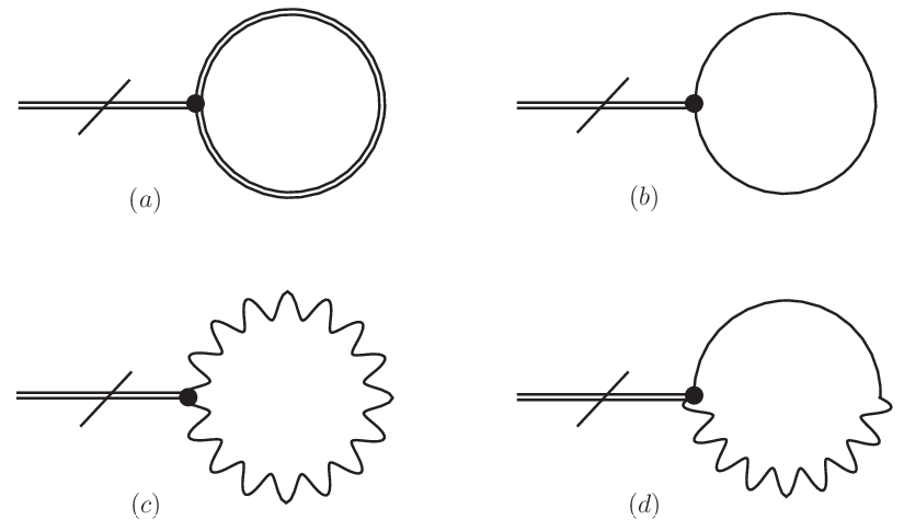
Inserting the superpropagators (17) into the expression above and integrating over $\theta$, one obtains

	$\displaystyle\Gamma_{1}^{(\Sigma)}$	$\displaystyle=$	$\displaystyle i\int d^{3}\widetilde{p}\frac{d^{3}k}{\left(2\pi\right)^{3}}\Bigl[\Bigl(e^{2}\sigma_{1}s_{1}\left(k\right)+eb_{5}\left(k\right)-2eb_{3}\left(k\right)-g\sigma_{1}a_{1}\left(k\right)-3g\sigma_{1}c_{1}\left(k\right)\Bigr)\widetilde{\Sigma}_{2}(p)+$		(28)
			$\displaystyle-\Bigl(-e^{2}\sigma_{2}s_{1}\left(k\right)+e^{2}\sigma_{1}s_{4}\left(k\right)+eb_{7}\left(k\right)+g\sigma_{2}a_{1}\left(k\right)-g\sigma_{1}a_{4}\left(k\right)$
			$\displaystyle+3g\sigma_{2}c_{1}\left(k\right)-3g\sigma_{1}c_{4}\left(k\right)\Bigr)\widetilde{\Sigma}_{1}(p)\Bigr].$

It is important to note that it was not necessary to consider the explicit form of the propagator coefficients in order to perform the Grassmann integration (i.e. the D-algebra). This is always possible since the propagator coefficients are merely functions on $k^{2}$ and the parameters of the shifted theory, while the D-algebra entails $(\theta_{\alpha},\,D_{\alpha},\,k_{\alpha\beta})$ manipulations which are explicit in the definitions of the bases (18-20).

To proceed, as was made in the tree-level case, we set up the tadpole equations by reading directly the $\Sigma_{1}\left(\Sigma_{2}\right)$ tadpoles from (28). This leads to

	$\displaystyle\frac{\partial U_{1}}{\partial\sigma_{1}}$	$\displaystyle=$	$\displaystyle i\int\frac{d^{3}k}{\left(2\pi\right)^{3}}\left[-e^{2}\sigma_{2}s_{1}\left(k\right)+e^{2}\sigma_{1}s_{4}\left(k\right)+eb_{7}\left(k\right)+g\sigma_{2}a_{1}\left(k\right)-g\sigma_{1}a_{4}\left(k\right)\right.$		(29)
			$\displaystyle\left.+3g\sigma_{2}c_{1}\left(k\right)-3g\sigma_{1}c_{4}\left(k\right)\right]$
	$\displaystyle\frac{\partial U_{1}}{\partial\sigma_{2}}$	$\displaystyle=$	$\displaystyle-i\int\frac{d^{3}k}{\left(2\pi\right)^{3}}\left[e^{2}\sigma_{1}s_{1}\left(k\right)+eb_{5}\left(k\right)-2eb_{3}\left(k\right)-g\sigma_{1}a_{1}\left(k\right)-3g\sigma_{1}c_{1}\left(k\right)\right],$		(30)

where the coefficients $\left\{a_{i},\,b_{i},\,c_{i},\,s_{i}\right\}$ are functions on $\sigma_{1}$ and $\sigma_{2}$ (see Appendix A ).

Solving this system of differential equations, the one-loop contribution (in the Landau gauge $\alpha=0$) is

	$\displaystyle U_{1}\left(\sigma_{i}\right)$	$\displaystyle=$	$\displaystyle\frac{\sigma_{1}\sigma_{2}}{4}i^{2}\int\frac{d^{3}k_{E}}{\left(2\pi\right)^{3}}\frac{-3e^{2}g^{3}\sigma_{1}^{8}\left(e^{2}-3g\right)-g\sigma_{1}^{4}\left(e^{4}-10e^{2}g+48g^{2}\right)k_{E}^{2}+\left(e^{2}-16g\right)k_{E}^{4}}{\left(k_{E}^{2}+\mu_{1}^{2}\right)\left(k_{E}^{2}+\mu_{2}^{2}\right)\left(k_{E}^{2}+\mu_{3}^{2}\right)}$		(31)
		$\displaystyle=$	$\displaystyle\frac{1}{64\pi}\left(e^{4}-160g^{2}\right)\sigma_{1}^{3}\sigma_{2}+\mathcal{O}\left(\sigma_{1},\,\sigma_{2}^{2}\right).$

Here $k_{E}$ represents the Euclidean momentum. As is seen from the sum of (21) and (31), neither the supersymmetry nor the internal $U\left(1\right)$ symmetry are broken up to this order.

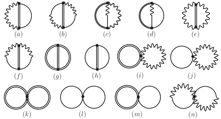
Now let us go to the two-loop approximation. In this order, the vacuum bubbles which contribute to the effective potential are displayed in Figure 2. Their respective integrals after performing the D-algebra, with the aid of the SusyMath package [21], are collected in Appendix B.

Using dimensional regularization to integrate over the internal momenta and specifically the formulas found in [22, 23], we obtain for the two-loop contribution the following result

$\displaystyle U_{2}\left(\sigma_{1},\sigma_{2}\right)$

$\displaystyle=$

$\displaystyle\frac{1}{512\pi^{2}}\left[\frac{2a_{1}}{\epsilon}+a_{2}-4a_{1}\ln\left(\frac{\sigma_{1}^{2}}{\mu}\right)\right]\sigma_{1}^{3}\sigma_{2}+B_{ct}\sigma_{1}^{3}\sigma_{2},$

(32)

where $\epsilon=3-D$ and $\mu$ is an arbitrary mass scale introduced in the dimensional regularization. The constant $B_{ct}$, chosen as $B_{ct}=-\frac{2a_{1}}{512\pi^{2}}$$\frac{1}{\epsilon}+B_{fin}$ is a tree-level counterterm to the coupling constant $g$ that will cancel the two-loop infinite and adjust the coupling constant to the required renormalization condition. The constants $a_{1}$ and $a_{2}$ are given by

$\displaystyle a_{1}$

$\displaystyle\doteq$

$\displaystyle e^{6}+7e^{4}g-16e^{2}g^{2}-1024g^{3},$

(33)

and

	$\displaystyle a_{2}$	$\displaystyle\doteq$	$\displaystyle a_{1\,}2\left(1-\gamma+\ln(4\pi)\right)+32g^{3}\left[-47\ln 2+243\ln 3+20\left(5+\ln 5\right)\right]+3936g^{3}\ln g$		(34)
			$\displaystyle+4e^{4}g\left(-5+\ln 256\right)+\left(4\ln 2-1\right)e^{6}-4\left(e^{2}-6g\right)\left(e^{2}+6g\right)^{2}\ln\left(e^{2}+6g\right)$
			$\displaystyle+16e^{2}g^{2}\left(\ln 2-5\right)+\left[12e^{4}g-144e^{2}g^{2}-1728g^{3}+e^{6}\right]\ln\left(e^{2}+12g\right)$
			$\displaystyle-\left(e^{2}-8g\right)\left(e^{2}+8g\right)\left(e^{2}+16g\right)\ln\left(e^{2}+16g\right),$

where $\gamma=0.5772\cdots$ is the Euler’s constant. Defining the constants

$$Y\left(e,g\right)\doteq\frac{a_{1}}{128\pi^{2}}\qquad\mbox{and}\qquad X\left(e,g\right)\doteq\frac{e^{4}-160g^{2}}{64\pi}+\frac{a_{2}}{512\pi^{2}}+B_{fin},$$

(35)

the effective potential up to two-loops (in the Landau gauge $\alpha\rightarrow 0$ and $\sigma_{2}$-linear approximation in the loop corrections) is given by the sum of (21), (31) and (32)

$\displaystyle U\left(\sigma_{1},\,\sigma_{2}\right)$

$\displaystyle=$

$\displaystyle-\frac{1}{2}\sigma_{2}^{2}+\left[g+X\left(e,g\right)-Y\left(e,g\right)\ln\frac{\sigma_{1}^{2}}{\mu}\right]\sigma_{1}^{3}\sigma_{2}+\mathcal{O}\left(\sigma_{1},\,\sigma_{2}^{2}\right).$

(36)

Eliminating the auxiliary field $\sigma_{2}$ by using its Euler-Lagrange equation $\partial U/\partial\sigma_{2}=0$ we get

$$\sigma_{2}(\sigma_{1})=\left[g+X\left(e,g\right)-Y\left(e,g\right)\ln\frac{\sigma_{1}^{2}}{\mu}\right]\sigma_{1}^{3},$$

(37)

which substituted in $U\left(\sigma_{1},\,\sigma_{2}\right)$ results in

$$U(\sigma_{1})=\frac{1}{2}\sigma_{2}^{2}(\sigma_{1})=\frac{\sigma_{1}^{6}}{2}\left[g+X\left(e,g\right)-Y\left(e,g\right)\ln\frac{\sigma_{1}^{2}}{\mu}\right]^{2}.$$

(38)

Besides the usual minimum at $\sigma_{1}=0$, this potential has a possible new minimum at $\sigma_{1}=\eta\neq 0$ satisfying $g+X\left(e,g\right)-Y\left(e,g\right)\ln\frac{\eta^{2}}{\mu}=0.$ By imposing the renormalization condition:

$$\left.\frac{\partial^{6}U}{\partial\sigma_{1}^{6}}\right|_{\sigma_{1}=\eta}=\frac{\partial^{6}U_{cl}}{\partial\sigma_{1}^{6}}=360g^{2},$$

(39)

we obtain the relation

$$\sqrt{\frac{45}{812}}g=Y=\frac{1}{128\pi^{2}}(e^{6}+e^{4}g+\cdots)$$

(40)

between the two coupling constants. Up to order $e^{6}\ll 1,$ this condition implies that $Y=\frac{e^{6}}{128\pi^{2}}=\sqrt{\frac{45}{812}}g.$ This is the Coleman-Weinberg condition that guarantees that the new minimum $\sigma_{1}=\eta$ is in the range of the perturbative calculations of our approach. In the renormalization process the constant $X\left(e,\,g\right)$ and the finite counterterm $B_{fin}$ get automatically fixed and disappear from the expression of $U_{ren}$. The dependence on logaritms of the coupling constants (present in $X$) completely disappeared from the result. The renormalized effective potential only relies on $Y$ which is a polynomial in the coupling constants. The result is

$$U_{ren}=\frac{Y^{2}}{2}\sigma_{1}^{6}\ln^{2}\left[\frac{\sigma_{1}^{2}}{\eta^{2}}\right].$$

(41)

The new minimum $\sigma_{1}=\eta$ implies in $\sigma_{2}=0=U_{ren}.$ This result means that supersymmetry is preserved but the gauge $U\left(1\right)$ symmetry is broken through a Higgs mechanism that is radiatively induced. In order to analyse the spectrum of the resulting quantum excitations we now restore the rotational symmetry by performing the substitution $\sigma_{1}^{2}\rightarrow\sigma_{1}^{2}+\pi_{1}^{2}$. The above potential becomes

$$U_{ren}(\sigma_{1},\,\pi_{1})=\frac{1}{2}\left[\frac{e^{6}}{128\pi^{2}}\right]^{2}(\sigma_{1}^{2}+\pi_{1}^{2})^{3}\,\ln^{2}\left[(\sigma_{1}^{2}+\pi_{1}^{2})/\eta^{2}\right].$$

(42)

A continuous set of new vacua are given by $\sigma_{1}^{2}+\pi_{1}^{2}=\eta^{2}.$ Let us choose the vacuum $\sigma_{1}=\eta$ and $\pi_{1}=0$. The quantum fields around this new vacuum present a Higgs mechanism [24]. The mass of the Higgs superfield $\Sigma$ and the Goldstone superfield $\Pi$ are got from the second derivatives of the effective potential at the vacuum:

$$m_{\Sigma}^{2}=\left.\frac{\partial^{2}U_{ren}}{\partial\sigma_{1}^{2}}\right|_{(\sigma_{1},\pi_{1})=(\eta,0)}=4\,\left[\frac{e^{6}}{128\pi^{2}}\right]^{2}\eta^{4}$$

(43)

$$m_{\Pi}^{2}=\left.\frac{\partial^{2}U_{ren}}{\partial\pi_{1}^{2}}\right|_{(\sigma_{1},\pi_{1})=(\eta,0)}=0$$

(44)

The mass generation for the gauge superfield $A_{\alpha}$ can be seen in the following way. After renormalization and restoration of the rotational symmetry, (36) becomes

$$U_{ren}=-\frac{1}{2}(\sigma_{2}^{2}+\pi_{2}^{2})-Y(\sigma_{1}\sigma_{2}+\pi_{1}\pi_{2})(\sigma_{1}^{2}+\pi_{1}^{2})\ln\left[(\sigma_{1}^{2}+\pi_{1}^{2})/\eta^{2}\right].$$

(45)

As shown above, the first term comes from the kinetic terms of $\Sigma$ and $\Pi$ in the action of (8). The second term replaces the classical interaction potential $U_{cl}=g(\sigma_{1}^{2}+\pi_{1}^{2})(\sigma_{1}\sigma_{2}+\pi_{1}\pi_{2})$ that, in turn, comes from the term

$$\delta S_{cl}=-\int d^{5}z\,\frac{g}{4}\left(\Sigma^{2}+\Pi^{2}\right)^{2}$$

(46)

in (8). In the same way, the second term of $U_{ren}$ in (45) can be obtained from

$$\delta S_{eff}=\int d^{5}z\,\frac{Y}{4}\,(\Sigma^{2}+\Pi^{2})^{2}\left\{\ln\left[(\Sigma^{2}+\Pi^{2})/\eta^{2}\right]+\frac{1}{2}\right\},$$

(47)

after shifting the fields by their classical expectation values $\sigma$ and $\pi$ and integrating in $d^{2}\theta$.

The effect of the radiative corrections is to change the classical potential by the effective one. Forgetting other possible radiative corrections to the kinetic terms, the effective action is then given by (8) with the classical interaction potential (46) substituted by the effective one (47). By doing the shift $\Sigma\longrightarrow\Sigma+\eta$ in this effective action, we see that a mass term $m_{A}A^{\alpha}A_{\alpha}/2$ with $m_{A}=e^{2}\eta^{2}/2$ is induced for the gauge superfield (besides the mass term $-\frac{1}{2}m_{\Sigma}\Sigma^{2}$ for $\Sigma$). Yet, a bilinear mixing term of the form $\frac{e}{2}\eta\Pi D_{\alpha}A^{\alpha}$ is also induced in the action. These two facts are features of the Higgs mechanism [24]: the gauge field combines with the “would-be” Goldstone scalar superfield, absorbing its degrees of freedom and becoming massive. In our case the originally non propagating gauge superfield $A_{\alpha}$ absorbs the degrees of freedom of the super-Goldstone field $\Pi$, becoming a massive propagating superfield.

References

- [1] E. Witten, Nucl. Phys. B188, 513 (1981).
- [2] M. T. Grisaru, M. Rocek, and W. Siegel, Nucl. Phys. B159, 429 (1979).
- [3] J. Bagger and N. Lambert, Phys. Rev. D 75, 045020 (2007); Phys. Rev. D 77, 065008 (2008); J. High Energy Phys. 02 (2008) 105; A. Gustavsson, J. High Energy Phys. 04 (2008) 083; Nucl. Phys. B811, 66 (2009).
- [4] O. Aharony, O. Bergman, D. L. Jafferis, and J. Maldacena, J. High Energy Phys. 10 (2008) 091.
- [5] M. van Raamsdonk, J. High Energy Phys. 05 (2008) 105.
- [6] S. V. Ketov and S. Kobayashi, Phys. Rev. D 83, 045003 (2011).
- [7] A. Mauri and A. C. Petkou, Phys. Lett. B 666, 527 (2008).
- [8] S. Deser, R. Jackiw and S. Templeton, Ann. Phys. 140, 372 (1982); Phys. Rev. Lett. 48, 975 (1982).
- [9] S. M. Girvin, in The quantum Hall effect, edited by R. E. Prange and S. M. Girvin, Springer-Verlag, New York (1990), 2nd ed.
- [10] F. Wilczek, Fractional statistics and anyon superconductivity, World Scientific, Singapore (1990).
- [11] S. Weinberg, Phys. Rev. D 7, 2887 (1973).
- [12] R. Jackiw, Phys. Rev. D 9, 1686 (1974).
- [13] J. L. Boldo, L. P. Colatto, M. A. De Andrade, O. M. Del Cima and J. A. Helayël-Neto, Phys. Lett. B 468, 96 (1999).
- [14] E. A. Gallegos and A. J. da Silva, Phys. Rev. D 84, 065009 (2011).
- [15] S. J. Gates, M. T. Grisaru, M. Rocek, and W. Siegel, Superspace or one thousand and one lessons in supersymmetry, Benjamin-Cummnings, Massachusetts (1983).
- [16] S. Coleman and E. Weinberg, Phys. Rev. D 7, 1888 (1973).
- [17] L. Alvarez-Gaumé, D. Z. Freedman and M. T. Grisaru, Harvard HUTMP No 81/B111, 1982; C. P. Burgess, Nucl. Phys. B 216, 459 (1983).
- [18] A. F. Ferrari, E. A. Gallegos, M. Gomes, A. C. Lehum, J. R. Nascimento, A. Yu. Petrov, and A. J. da Silva, Phys. Rev. D 82, 025002 (2010); A. C. Lehum and A. J. da Silva, Phys. Lett. B, 693, 393 (2010).
- [19] L. Dolan and R. Jackiw, Phys. Rev. D 9, 2904 (1974).
- [20] N. K. Nielsen, Nucl. Phys. B101, 173 (1975); I. J. R. Aitchison and C. M. Fraser, Ann. of Phys. (N.Y.) 156, 1 (1984); D. Johnston, Nucl. Phys. B253, 687 (1985).
- [21] A. F. Ferrari, Comput. Phys. Commun. 176, 334 (2007).
- [22] P. N. Tan, B. Tekin, and Y. Hosotani, Phys. Lett. B 388, 611 (1996); Nucl. Phys. B502, 483 (1997).
- [23] A. G. Dias, M. Gomes, and A. J. da Silva, Phys. Rev. D 69, 065011 (2004).
- [24] F. Englert and R. Brout, Phys. Rev. Lett. 13, 321 (1964); P. Higgs, Phys. Lett. 12, 132 (1964); G. S. Guralnik, C. R. Hagen, and T. W. B. Kibble, Phys. Rev. Lett. 13, 585 (1964); P. Higgs, Phys. Rev. 145, 1156 (1966); T. W. B. Kibble, ibid. 155, 1554 (1967).