Mean-field Density Functional Theory of a Three-Phase Contact Line

In this paper, we treat a ternary system under the constraint of constant and uniform total molar volume. We obtain a tractable problem by introducing an explicit potential that is symmetric with respect to the three chemical components.

For a ternary system, $c=3$. Under the simplifying constraint of constant total molar volume,

With this constraint, the system we treat is actually a pseudo-binary system that can be described by two independent concentrations, say $\rho_{1}$ and $\rho_{2}$. Moreover, this constraint means that the conjugate thermodynamic variables of $\rho_{1}$ and $\rho_{2}$ are the chemical potential differences $M_{1}=\mu_{1}-\mu_{3}$ and $M_{2}=\mu_{2}-\mu_{3}$, where the $\mu_{i}$ would correspond to a system with variable molar volume. In symmetric form, our potential is

where $B$ is constant with the units of energy per unit volume, and $\rho_{a}$ and $\rho_{b}$ are parameters (units of concentration), which may depend on $T$ and the $M_{i}$. By imposing the constraint $\rho_{a}+2\rho_{b}=\rho$, we locate the three wells at symmetric positions.

We introduce the notation $X_{i}\equiv\rho_{i}/\rho$ as the mole fraction of chemical constituent $i$ ranging from 0 to 1, $a=\rho_{a}/\rho$, and $b=\rho_{b}/\rho=(1-a)/2$. The constraint (11) reduces to $X_{1}+X_{2}+X_{3}=1$. The potential (12) can be expressed as

The function $f(X_{1},X_{2},X_{3})$ was originally introduced by Eldred [36]. In terms of independent variables, one has a two-variable function,

The combination of $(X_{1},X_{2},X_{3})$ can be illustrated by a point in the Gibbs triangle as shown in Fig. 2. The compositions of the bulk phases are $(a,b,b)$, $(b,a,b)$, and $(b,b,a)$. When $a>1/3$, the three minima are located between vertices and the center of the Gibbs triangle, as illustrated in Fig. 3(a). The potential has a local maximum at $X_{1}=X_{2}=X_{3}=1/3$. For $a<1/3$, the three minima are rotated by $30^{\circ}$ to positions between mid edges and the center of the Gibbs triangle, as illustrated in Fig. 3(b).

In the reduced approximation (10) of $\psi(\mathbf{x})$, we assume that the gradient energy density is a linear function of the squares of the gradients of the mole fractions of each chemical component:

where $\ell_{i}$ are positive constants (with dimensions of length) associated with each chemical component. With the constraint $\nabla X_{3}=-\nabla X_{1}-\nabla X_{2}$, the form (15) of gradient energy density turns into a two-variable function,

Thus, by inserting the explicit forms of potential (13) and gradient energy density (15) into the form (10) of $\psi(\mathbf{x})$, the excess grand potential in our model (5) becomes

In equilibrium, we require $\delta\Omega_{xs}=0$ for infinitesimal variations of $X_{1}$ and $X_{2}$. To constrain total mole number of a finite system, we could add two Lagrange multipliers for $X_{1}$ and $X_{2}$ to the integrand. However, we effectively work on an open system with infinite domain and fixed parameters $\mu_{i}$ and $T$, so particle conservation is not an issue and the Lagrange multipliers are effectively zero. From another point of view, the bulk phase is reached when the distance from the three-phase contact line to the boundary is large compared to the diffuse region of the contact line. This implies that the mole fractions should satisfy the boundary condition $\nabla X_{i}\cdot\hat{n}=0$, where $\hat{n}$ is the unit outward normal to the physical domain. Thus, we obtain two coupled Euler-Lagrange equations

In order to make a connection with the sharp interface limit of our mean-field density model, we consider a transition from phase $\beta$ to phase $\alpha$ in the far-field regime, which is far from the three-phase contact line relative to the interfacial width. This is illustrated in Fig. 4, which corresponds to the transition from the minimum of one well to the minimum of another. Consistent with our potential function, $X_{3}=b$ is a constant in this region, which also satisfies the boundary condition $\nabla X_{3}\cdot\hat{n}=0$. Therefore, the problem is essentially a one dimensional problem in a single variable, which we take to be $X_{1}$.

With $X_{3}=b$, we replace $X_{2}=1-b-X_{1}$, and substitute $\nabla^{2}X_{i}=\mathrm{d}^{2}X_{i}/\mathrm{d}s^{2}$ in the form of (17) of excess grand potential, where $s$ is a coordinate perpendicular to the $\alpha\beta$-interface measured from $\beta$ to $\alpha$. The excess grand potential in the far field regime reduces to

where $w$ is the width of an area in the far field regime as indicated in Fig. 4, $H(X_{1})\equiv 2(X_{1}-a)^{2}(X_{1}-b)^{2}$, and $\alpha_{12}\equiv\ell_{1}^{2}+\ell_{2}^{2}$. The limits of integration are effectively from $-\infty$ to $\infty$.

In equilibrium, we require $\delta\Omega_{xs}=0$ for an infinitesimal variation of $X_{1}$ and obtain the Euler-Lagrange equation in the far-field limit:

Then, we multiply by $\mathrm{d}X_{1}/\mathrm{d}s$ and integrate to obtain

where the integration constant is zero because $H(a)=H(b)=0$ and the slope $\mathrm{d}X_{1}/\mathrm{d}s$ is zero for $X_{1}=a$ and $X_{1}=b$.

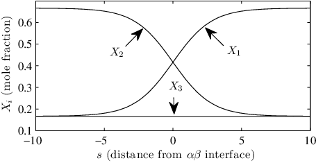
By solving (21), we obtain the far-field solution for $X_{1}$ at the $\alpha\beta$-interface,

where we choose $s=0$ as $X_{1}=(a+b)/2$ and define the interfacial width parameter of the $\alpha\beta$-interface as

Of course, $X_{2}=1-b-X_{1}$. These analytic solutions were originally found by Eldred [36]. Analytical far-field solutions for density profiles and interfacial tensions for a symmetric three-phase contact line but a different potential were obtained by Szleifer and Widom [7]. Note that when $a=b=1/3$, the interfacial widths diverge. The contact line and the three interfaces vanish. In this case, the three chemical constituents have mole fractions of $1/3$ distributed uniformly over the entire system.

As illustrated in Fig. 5, when $s$ is negative infinity, we have $X_{1}=b$ and $X_{2}=a$, which indicates the $\beta$ bulk phase. In contrast, when $s$ is positive infinity, we obtain $X_{1}=a$ and $X_{2}=b$, which refers to the $\alpha$ bulk phase. Similarly, we can apply the same analysis for the other two interfaces and obtain solutions for $X_{1}$, $X_{2}$, and $X_{3}$ in the far-field limit.

The definition of interfacial tension is the excess grand potential per unit area of interface. Thus, by inserting the relation (21) that connects potential and gradient density into the excess grand potential (19), the interfacial tension of the $\alpha\beta$-interface can be expressed as

After integration, the interfacial tension of the $\alpha\beta$-interface is found to be

The interfacial tensions of the $\beta\gamma$-interface and the $\gamma\alpha$-interface can be obtained similarly. Consistent with the classical relation of equilibrium angles (1), the equilibrium angles in our model obey

To discretize the Euler-Lagrange equations (29), for a symmetric three-phase contact line based on the triangular grid in Fig. 6, we employ a variation of the discrete form of the excess grand potential to avoid inconsistent discretization of the potential of $f$ and the gradient energy $g$. We approximate $u$ and $v$ as planer functions in the region of each small triangle of the triangular grid. Then, the value of $u$ and $v$ at the central point $n$ is defined as $u_{n}\equiv\sum_{m\in V^{(n)}}u_{m}/3$ and $\sum_{m\in V^{(n)}}v_{m}/3$, where $V^{(n)}$ is the set of vertices of the small triangle denoted by its center point $n$ (see Fig. 7). The discrete form of the dimensionless excess grand potential (17) is approximated by evaluating the integrand at the central point of each small triangle,

where $CP$ is the set of the central points of the small triangles over the entire triangular grid in Fig. 6; $\Delta$ is the area of each small triangle; $f_{n}\equiv f(u_{n},v_{n})$ and $\bar{g}_{n}\equiv\bar{g}((\nabla^{\prime}u)_{n},(\nabla^{\prime}v)_{n})$. Since $u$ and $v$ are approximated by planer functions, we obtain

where $PV^{(n)}$ is the set of pairs of the vertices $V^{(n)}$ (Fig. 7) of the small triangle $n$ with edge $d^{\prime}$.

At equilibrium, we require $\delta\Omega_{xs}^{\prime}=0$ for the discrete form (31) of the excess grand potential. From the chain rule, this is equivalent to the vanishing of the sum of the variations of all of the unknowns $(u_{i},v_{i})$ for each internal site $i$ of the triangular grid. According to the approximations (32) of the gradient energy density and requiring the coefficients of $\delta u_{i}$ and $\delta v_{i}$ to vanish, we obtain the discrete Euler-Lagrange equations for each site $i$ (each internal grid point of the triangular grid),

where $\overline{\left(\partial f/\partial u\right)}_{NCP^{(i)}}\equiv\sum_{n\in NCP^{(i)}}(\partial f/\partial u)_{n}/6$ and $\overline{\left(\partial f/\partial v\right)}_{NCP^{(i)}}\equiv\sum_{n\in NCP^{(i)}}(\partial f/\partial v)_{n}/6$ are the averages of $\partial f/\partial u$ and $\partial f/\partial v$ over the six nearest center points of each site $i$, $NCP^{(i)}$ (Fig. 7). The approximate Laplacian operators according to second order Taylor’s series expansions are $(\nabla^{\prime 2}u)_{i}\equiv 4(\overline{u}_{NN^{(i)}}-u_{i})/d^{\prime 2}$ and $(\nabla^{\prime 2}v)_{i}\equiv 4(\overline{v}_{NN^{(i)}}-v_{i})/d^{\prime 2}$, where $\overline{u}_{NN^{(i)}}\equiv\sum_{m\in NN^{(i)}}u_{m}/6$ and $\overline{v}_{NN^{(i)}}\equiv\sum_{m\in NN^{(i)}}v_{m}/6$ are the averages of $u$ and $v$ over the six nearest neighbors of each site $i$, $NN^{(i)}$ (Fig. 7).

Note that the discrete Euler-Lagrange equations (33) are similar to the analytic form (29), except $\partial f/\partial X_{1}$ and $\partial f/\partial X_{2}$ are replaced by the average values over the six nearest central points. After we apply the asymptotic far-field solutions as the boundary conditions of the system of algebraic equations for the triangular grid, there are $(N-2)(N-3)$ algebraic equations for the whole domain.

To solve the system of coupled algebraic equations, we apply the method of successive over-relaxation (SOR) [37, 38]. We define error equations for the diagonalized form of the discrete Euler-Lagrange equations (33):

where $0\leq\lambda\leq 1$ is an adjustable parameter used to implement our numerical technique, and $(r_{u})_{i}$ and $(r_{v})_{i}$ are the residues that we try to make as small as practical.

In the form (34) of error equations, $\overline{\left(\partial f/\partial u\right)}_{NCP^{(i)}}$ and $\overline{\left(\partial f/\partial v\right)}_{NCP^{(i)}}$ are polynomials of the mole fractions. To avoid the complexity of numerical calculation due to the nonlinearity of these terms, at the beginning, $\lambda$ is set to be zero. After solving this simplest version of the equation by SOR, we apply that solution as the initial values of SOR for new equations in which $\lambda$ is increased by a small fraction of 1, and solve the equations again. Then, we gradually enlarge $\lambda$ and repeat this procedure until $\lambda$ reaches one.

In the updating process of SOR, we first input guessed numbers of $u_{i}$ and $v_{i}$ as initial values into error equations (34) for every site in the grid. Then, we update $u_{i}$ and $v_{i}$ for each site by

where $q=1.86$ [39]. We repeat this procedure until the values of $u_{i}$ and $v_{i}$ at every site converge.

To check convergence, we study the norm of errors after every iteration. The norms are defined as

Then the convergence criteria can be defined as $\left\|r_{u}\right\|$ and $\left\|r_{v}\right\|$ are simultaneously smaller than $\epsilon$, where $\epsilon$ is a small number. Alternatively, this means $\left\|u_{i}^{new}-u_{i}^{old}\right\|$ and $\left\|v_{i}^{new}-v_{i}^{old}\right\|$ are simultaneously smaller than $qd^{\prime 2}\epsilon/4$.

Here, we present a numerical solution obtained from SOR. The numerical input is $a=2/3$, $d^{\prime}=0.1$, and $m=180$. The error tolerance, $\epsilon$, is $10^{-8}$. Then the domain edge $H^{\prime}=108$ is large compared to the interfacial width parameter $\delta_{int}^{\prime}=2\sqrt{2}$. Solutions for $X_{2}$ and $X_{3}$ are just the rotation of the solution of $X_{1}$ by $120^{\circ}$ and $240^{\circ}$. The solution for $X_{1}$ in Fig. 8(a) reveals the nature of diffuse interfaces. There is bending and slight widening of the diffuse region for $X_{1}$ near the three-phase contact line, which is quantified by the interfacial width defined from $10\%$ to $90\%$ isoconcentration lines. The width at the boundary, $\delta^{\prime}_{10\%-90\%,b}$, is about $6.21\approx 2.20\delta_{int}^{\prime}$. For comparison, the width at the contact line, $\delta^{\prime}_{10\%-90\%,t}\approx 7.37\approx 2.61\delta_{int}^{\prime}$, is about $20\%$ larger. $\delta^{\prime}_{10\%-90\%,t}$ is small compared to the distance from the outer domain boundary to the contact line along any interface, which is $R^{\prime}\approx 31.2\approx 11.0\delta_{int}^{\prime}$. Also, the profile at the contact line shifts its center compared to the one at the boundary, as shown in Fig. 8(b). Close to the boundary, the nearly parallel isoconcentration lines along the interfaces show that our domain size is close to the asymptotic regime, consistent with our intended boundary condition.

The numerical results in Sec. III reveal the fact that the actual interfacial width increases slightly while approaching the three-phase contact line. This result is different than that which would be obtained by extrapolation of the far-field solution. In this section, we study the line tension which is the excess energy per unit length associated with the three-phase contact line. By convention, the line tension is defined in the form (4) of the excess grand potential. For a symmetric contact line, we let $R\equiv R_{\alpha\beta}=R_{\beta\gamma}=R_{\gamma\alpha}$, and $\sigma\equiv\sigma_{\alpha\beta}=\sigma_{\beta\gamma}=\sigma_{\gamma\alpha}$. In terms of the dimensionless grand potential (27) with $R^{\prime}\equiv R/\ell$, the dimensionless line tension is given by

where $\sigma^{\prime}$ is the dimensionless form of the interfacial tension in the far-field limit (25) for a symmetric contact line, i.e.

From the symmetry of $\psi(\mathbf{x})$ for a symmetric contact line, the solutions for the three mole fractions have the property $X_{1}(r,\theta)=X_{2}(r,\theta-\frac{2\pi}{3})=X_{3}(r,\theta+\frac{2\pi}{3})$, which means each of them are given by only a rotation of $2\pi/3$ or $-2\pi/3$ from the others. Thus, the integration in the form (17) of excess grand potential can be divided into three equal parts. By applying the boundary condition $\nabla^{\prime}X\cdot\hat{n}=0$, we find that $\int\frac{1}{2}\left|\nabla^{\prime}X_{1}\right|^{2}\mathrm{d}A^{\prime}=-\int\frac{1}{2}X_{1}\nabla^{\prime 2}X_{1}\mathrm{d}A^{\prime}$. Thus, the dimensionless line tension is given by

We find, however, that evaluation of the form (39) of dimensionless line tension is sensitive to the choice of boundary condition, which may result from the inconsistency between the numerical evaluation of the excess grand potential and the analytic interfacial tension. Instead, we use a formula for line tension derived by Kerins and Boiteux [40], which transfers the second term of the form (39) of line tension into a surface integral and combines it with the first term. In this integral form, the integrands will vanish at distances far from the three-phase contact line, which means it is insensitive to domain size for a sufficiently large domain. According to the Kerins-Boiteux formula, the dimensionless line tension in given by

Numerically, we can discretize the integral in Eq. (40) by employing a triangular grid as in Fig. 6, so

where $f_{n}$ and $\bar{g}_{n}$ are defined in the discrete form (31) of the excess grand potential and the approximation (32) of the gradient energy density. Then we can utilize the numerical method developed in Sec. III to obtain the numerical value of dimensionless line tension in our model.

We perform a numerical evaluation of the integrand of the discrete form (41) of the Kerins-Boiteux formula. Fig. 9 shows a contour plot of the integrand on a logarithmic scale. A similar plot on a normal scale can be found in Taylor and Widom [35]. The integrand decays exponentially for the most of the domain. The major contribution of the integrand is approximately within the range from $10^{-2}$ to $10^{-5}$ at a core region centered at the three-phase contact line with dimension of $2$ to $3$ times $\delta_{int}^{\prime}$. The minor contribution, which is considered to be from $10^{-5}$ to $10^{-8}$, is distributed outside the core region and along the three interfaces with a width of about $1.5\delta_{int}^{\prime}$. The integrand in the rest of the domain is less than $10^{-8}$ and is essentially negligible compared to the one close to contact line and along the three interfaces. Theoretically, the potential and gradient energy density are zero within bulk phases and $-f+g\rightarrow 0$ in the interfaces far from the core, so the small but non-vanishing values of $-f+g$ along the interfaces results from numerical errors. Also, we can see that the contours of the integrand begin to bend at the far-field boundary of the domain, which may relate to the errors associated with applying the far-field solution as the boundary condition for a finite domain. Note that the contours along the three interfaces are nearly parallel except close to the contact line and the boundary. This suggests that the numerical evaluation of the Kerins-Boiteux integral over these areas leads to an error that is approximately proportional to $R^{\prime}$. Our numerical results also show that when $d^{\prime}$ is smaller, the distribution of the integrand within the core region is sharper, with a slightly larger maximum value, and decays faster, which means that the integrands along the three interfaces and the boundary decrease when $d^{\prime}$ becomes smaller. So, we assume that the numerical error of the evaluation of the Kerins-Boiteux formula is proportional to $R^{\prime}$ and depends on $d^{\prime}$.

To test this, we use the Kerins-Boiteux formula to calculate values of line tension, $\tau^{\prime}$. As shown in Fig. 10, the $\tau^{\prime}$ value is nearly proportional to $R^{\prime}$ for each $d^{\prime}$. We take grid spacings, $d^{\prime}=0.05$, $0.1$, $0.2$, and $0.4$, and domain sizes, $R^{\prime}\approx 31.2$, $41.2$, $52.0$, and $62.4$, which are relatively large compared to the size of the three-phase contact line, roughly $7.37\approx 2.61\delta_{int}^{\prime}$. By linear extrapolation from the results in Fig. 10, we find that the values of $\tau^{\prime}$ for different $d^{\prime}$ roughly meet at $R^{\prime}=0$. Moreover, from Fig. 11, we find that the dominant numerical error of $\tau^{\prime}$ comes from a $d^{\prime 2}$ term for fixed $R^{\prime}$ values because the calculated $\tau^{\prime}$ is almost linear in $d^{\prime 2}$.

On the basis of Fig. 10 and Fig. 11, we assume that the numerical value of $\tau^{\prime}$ is a function of $R^{\prime}$ and $d^{\prime}$ of the form

where $c_{1}$ and $c_{2}$ are constants, $\bar{\tau}^{\prime}$ is the line tension nearly invariant of the grid spacing $d^{\prime}$ and distance $R^{\prime}$, and $h(d^{\prime 2},R^{\prime})$ represents terms of higher order than $d^{\prime 2}$ and $R^{\prime}$. From the expression (42) of the numerical line tension $\tau^{\prime}(R^{\prime},d^{\prime})$, we can eliminate approximately the numerical error which depends on $R^{\prime}$ by linear extrapolation of $\tau^{\prime}$ from various $R^{\prime}$ toward $R^{\prime}=0$ as in Fig. 10 and obtain a correction of $\tau^{\prime}$ at $R^{\prime}=0$ , which is given by

where $h_{0}(d^{\prime 2})$ represents terms of higher order than $d^{\prime 2}$. The extrapolated results of $\tau^{\prime}_{0}$ (43) are listed in Table 1.

In addition, we can refine our result at $R^{\prime}=0$ by using Richardson’s extrapolation [41, 42], in which results for two successive $d^{\prime}$ values are used to eliminate the $d^{\prime 2}$ term. The first level of correction is defined as

where $h_{1}(d^{\prime 2})$ represents the terms of higher order than $d^{\prime 2}$. From the calculation of $\tau^{\prime}_{1}$ in Table 1, the line tension $\tau^{\prime}$ for $a=2/3$ is approximated by

where the uncertainty is in the final digit. It is well known both theoretically [27, 43] and experimentally [1, 21] that line tensions, unlike interfacial tensions, can be either positive or negative. Physically, a negative line tension means, for example, that the line of intersection of a sessile drop with a substrate would tend to expand [1, 44], but is ultimately limited by positive interfacial tensions.

In our original way of scaling, we factored out $B\ell^{2}$ from the excess grand potential and also from the Kerins-Boiteux formula for line tension. Then, we calculated the integral in a dimensionless domain. However, our potential is parametrized by $a$, which means that solutions of the Euler-Lagrange equations and the calculation of $\tau^{\prime}$ depend on $a$. Here, to elucidate the $a$-dependence of our model, we study the problem in a new framework by defining the following new scaled variables,

where $\sum_{i=1}^{3}Y_{i}=1$ and $a\neq 1/3$. In our model, the value of $X_{i}$ is limited from $b$ to $a$, so $Y_{i}$ varies from 0 to 1. In terms of the new scaling variables, the new dimensionless form of the excess grand potential (17) for a symmetric three-phase contact line is given by

where we define the following new scaled constants $\tilde{B}\equiv B(a-b)^{4}$, $\tilde{\ell}^{2}\equiv\ell^{2}/(a-b)^{2}$, $\tilde{\nabla}\equiv\tilde{\ell}\nabla$, $\tilde{A}\equiv A/\ell^{2}$. The scaled potential and gradient energy density are