Quantitative Analysis of Information Leakage in
Probabilistic and Nondeterministic Systems
Miguel E. Andrés
Copyright © 2011 Miguel E. Andrés.
ISBN: 978-94-91211-74-4.
IPA dissertation series: 2011-09.
This thesis is typeset using LaTeX.
Translation of the Dutch summary: Peter van Rossum.
Cover designed by Marieke Meijer - www.mariekemeijer.com.
Thesis printed by Ipskamp Drukers - www.ipskampdrukkers.nl.
![[Uncaptioned image]](1111.2760v1/radboud.png)
![[Uncaptioned image]](1111.2760v1/inria.png)
![[Uncaptioned image]](1111.2760v1/ipa_white_300x200.png)
![[Uncaptioned image]](1111.2760v1/NWO_logo.png)
The work in this thesis has been carried out at Radboud University and under the auspices of the research school IPA (Institute for Programming research and Algorithmics). The research funding was provided by the NWO Grant through the open project 612.000.526: Analysis of Anonymity. The author also wishes to acknowledge the French Institute for Research in Computer Science and Control (INRIA) for providing funding for several research visits to the École Polytechnique of Paris.
Quantitative Analysis of Information Leakage in
Probabilistic and Nondeterministic Systems
Een wetenschappelijke proeve op het gebied van de Natuurwetenschappen, Wiskunde en Informatica.
Proefschrift
ter verkrijging van de graad van doctor
aan de Radboud Universiteit Nijmegen
op gezag van de rector magnificus, prof. mr. S.C.J.J. Kortmann,
volgens besluit van het College van Decanen
in het openbaar te verdedigen op vrijdag 1 juli 2011
om 10:30 uur precies
door
Miguel E. Andrés
geboren op 02 July 1980,
te Río Cuarto, Córdoba, Argentinië.
Promotor:
| prof. dr. Bart P.F. Jacobs |
Copromotoren:
| dr. Peter van Rossum |
| dr. Catuscia Palamidessi INRIA |
Manuscriptcommissie:
| prof. dr. Joost-Pieter Katoen | RWTH Aachen University |
| dr. Pedro R. D’Argenio | Universidad Nacional de Córdoba |
| prof. dr. Frits W. Vaandrager | |
| prof. dr. Holger Hermanns | Saarland University |
| dr. Mariëlle Stoelinga | University of Twente |
Quantitative Analysis of Information Leakage in
Probabilistic and Nondeterministic Systems
A scientific essay in Science.
Doctoral thesis
to obtain the degree of doctor
from Radboud University Nijmegen
on the authority of the Rector Magnificus, Prof. dr. S.C.J.J. Kortmann,
according to the decision of the Council of Deans
to be defended in public on Friday, 1 July 2011
at 10:30 hours
by
Miguel E. Andrés
born in Río Cuarto, Córdoba, Argentina
on 02 July 1980.
Supervisor:
| prof. dr. Bart P.F. Jacobs |
Co-supervisors:
| dr. Peter van Rossum |
| dr. Catuscia Palamidessi INRIA |
Doctoral Thesis Committee:
| prof. dr. Joost-Pieter Katoen | RWTH Aachen University |
| dr. Pedro R. D’Argenio | Universidad Nacional de Córdoba |
| prof. dr. Frits W. Vaandrager | |
| prof. dr. Holger Hermanns | Saarland University |
| dr. Mariëlle Stoelinga | University of Twente |
Summary
As we dive into the digital era, there is growing concern about the amount of personal digital information that is being gathered about us. Websites often track people’s browsing behavior, health care insurers gather medical data, and many smartphones and navigation systems store or transmit information that makes it possible to track the physical location of their users at any time. Hence, anonymity, and privacy in general, are increasingly at stake. Anonymity protocols counter this concern by offering anonymous communication over the Internet. To ensure the correctness of such protocols, which are often extremely complex, a rigorous framework is needed in which anonymity properties can be expressed, analyzed, and ultimately verified. Formal methods provide a set of mathematical techniques that allow us to rigorously specify and verify anonymity properties.
This thesis addresses the foundational aspects of formal methods for applications in security and in particular in anonymity. More concretely, we develop frameworks for the specification of anonymity properties and propose algorithms for their verification. Since in practice anonymity protocols always leak some information, we focus on quantitative properties which capture the amount of information leaked by a protocol.
We start our research on anonymity from its very foundations, namely conditional probabilities – these are the key ingredient of most quantitative anonymity properties. In Chapter 2 we present cpCTL, the first temporal logic making it possible to specify conditional probabilities. In addition, we present an algorithm to verify cpCTL formulas in a model-checking fashion. This logic, together with the model-checker, allows us to specify and verify quantitative anonymity properties over complex systems where probabilistic and nondeterministic behavior may coexist.
We then turn our attention to more practical grounds: the constructions of algorithms to compute information leakage. More precisely, in Chapter 3 we present polynomial algorithms to compute the (information-theoretic) leakage of several kinds of fully probabilistic protocols (i.e. protocols without nondeterministic behavior). The techniques presented in this chapter are the first ones enabling the computation of (information-theoretic) leakage in interactive protocols.
In Chapter 4 we attack a well known problem in distributed anonymity protocols, namely full-information scheduling. To overcome this problem, we propose an alternative definition of schedulers together with several new definitions of anonymity (varying according to the attacker’s power), and revise the famous definition of strong-anonymity from the literature. Furthermore, we provide a technique to verify that a distributed protocol satisfies some of the proposed definitions.
In Chapter 5 we provide (counterexample-based) techniques to debug complex systems, allowing for the detection of flaws in security protocols. Finally, in Chapter 6 we briefly discuss extensions to the frameworks and techniques proposed in Chapters 3 and 4.
Acknowledgements
This thesis would not have been possible without the continuous support of many people to whom I will always be grateful.
I am heartily thankful to my supervisor Bart Jacobs. He has closely followed the evolution of my PhD and made sure I always had all the resources a PhD student could possibly need.
I owe my deepest gratitude to my co-supervisor, Peter van Rossum. Four years have passed since he decided to take the risk to hire me, an Argentinian guy that he barely knew. I was really lucky to have Peter as my supervisor; he has always been very supportive, flexible, and extremely easygoing with me. I will never forget the football World Cup of (not that Argentina did very well); back then I was invited to spend one week in Nijmegen for an official job interview. But before I had the time to stress too much about formal talks and difficult questions, I found myself sharing a beer with Peter while watching Argentina vs the Netherlands (fortunately Argentina did not win — I still wonder what would have happened otherwise). This was just the first of many nice moments we shared together, including dinners, conversations, and trips. In addition to having fun, we have worked hard together — indeed we completed one of the most important proofs of this thesis at midnight after a long working day at Peter’s house (and also after Mariëlle finally managed to get little Quinten to sleep ).
I cannot allow myself to continue this letter without mentioning Catuscia Palamidessi. Much has changed in my life since I first met her in June 2007. Catuscia came then to visit our group in Nijmegen and we discovered that we had many research interests in common. Soon after, Catuscia invited me to visit her group in Paris and this turned out to be the beginning of a very fruitful collaboration. Since then we have spent countless days (and especially nights) working very hard together, writing many articles, and attending many conferences — including some in amazing places like Australia, Barbados, and Cyprus. Catuscia is not only an exceptionally bright and passionate scientist, but she is also one of the most thoughtful people I have ever met (placing the interests of her colleagues and PhD students above her own), a wonderful person to work with (turning every work meeting into a relaxed intellectual discussion, enhanced with the finest caffè italiano), and, above all, an unconditional friend. For these reasons and many more (whose enumeration would require a second volume for this thesis), I am forever indebted to Catuscia.
This work has also greatly benefited from the insightful remarks and suggestions of the members of the reading committee Joost-Pieter Katoen, Pedro D’Argenio, and Frits Vaandrager, whom I wish to thank heartily. To Pedro I am also grateful for his sustained guidance and support in my life as a researcher. Many results in this thesis are a product of joint work, and apart from Peter and Catuscia, I am grateful to my co-authors Mário S. Alvim, Pedro R. D’Argenio, Geoffrey Smith and Ana Sokolova, all of whom shared their expertise with me. I am also thankful to Jasper Berendsen, Domingo Gómez, David Jansen, Mariëlle Stoelinga, Tingting Han, Sergio Giro, Jérémy Dubreil, and Konstantinos Chatizikokolakis for many fruitful discussions during my time as a PhD student. Also many thanks to Anne-Lise Laurain for her constant (emotional and technical) support during the writing of my thesis, Alexandra Silva for her insightful comments on the introduction of this work, and Marieke Meijer for devoting her artistic talent to the design of the cover of this thesis.
Special thanks to my paranymphs and dear friends Vicenç, Igor, Cristina, and Flavio. Together we have shared so much… uncountable lunches in the Refter, coffees in the blue coaches, and trips around the world among many more experiences. But, even more importantly, we have always been there to support each other in difficult times, and this is worth the world to me.
I wish to thank my colleagues in the DS group for providing such a friendly atmosphere which contributed greatly to the realization of my PhD. I explicitly want to thank Alejandro, Ana, Chris, Christian, Erik, Fabian, Gerhard, Ichiro, Jorik, Ken, Łukasz, Olha, Pieter, Pim, Roel, Thanh Son, and Wojciech with whom I have shared many coffees, nice conversations, table tennis, and much more. My journey in the DS group would not have been as easy if it was not for Maria and Desiree whose help on administrative issues saved me lots of pain; as for any kind of technical problem or just IT advice, Ronny and Engelbert have been always very helpful.
I also wish to thank all the members of the Comète group for making me feel welcome in such a wonderful and fun group. In particular, I want to thank the Colombian crowd – Frank, Andrés, and Luis – for the nice nights out to “La Peña” and all the fun we had together, Jérémy for introducing me to the tennis group, Sophia for helping correct my English in this thesis, Kostas for many interesting conversations on the most diverse topics of computer science (and life in general), and Mário for finally acknowledging the superiority of the Argentinian soccer over the Brazilian one .
Along the years, I always had a very happy and social life in Nijmegen. Many people, in addition to my paranymphs, have greatly contributed to this. A very big thanks to “Anita”, for so many happy moments and her unconditional support during my life in Nijmegen. Also many thanks to my dear friend Renée, every time I hear “It is difficult to become friends with Dutch people, but once they are your friends they would NEVER let you down” I have to think of her. Special thanks to Elena and Clara for being there for me when I could not even speak English, Errez for sharing his wisdom in hunting matters , Hilje and Daphne for being there for me when I just arrived to Nijmegen (this was very important to me), also thanks to Klasien, David, and Patricia for many nice nights out and to my dear neighbours – Marleen, Kim, and Marianne – for welcoming me in their house and being always so understanding with me. Besides, I would like to thank to the “Blonde Pater crowd” including Cristina, Christian, Daniela, Davide, Deniz, Francesco, Jordan, Mariam, Nina, Shankar, and Vicenç with all of whom I shared many nice cappuccinos, conversations, and nights out. Special thanks to the sweet Nina for being always willing help me, to Francesco for the wonderful guitar nights, to Mariam for her help in Dutch, and to Christian… well, simply for his “buena onda”.
More than four years have passed since I left Argentina, and many things have certainly changed in my life. However, the support and affection of my lifetime friends have remained immutable. Many thanks to Duro, Seba, Tony, Viole, Gabi, and Martín for all they have contributed to my life. Special thanks to my “brothers” Tincho and Lapin, my life would not be the same without them.
Last but not least, all my affection to my family: dad Miguel, mum Bacho, sister Josefina, and brothers Ignacio and Augusto. Every single success in my life I owe mostly to them. Thanks to my brothers and sister for their constant support and everlasting smiles, which mean to me more than I can express in words. Thanks to my parents for their incessant and selfless sacrifice, thanks to which their children have had all anybody could possible require to be happy and successful. My parents are the greatest role models for me and to them I dedicate this thesis.
To my dear parents, Miguel and Bacho.
Por último, el “gracias” mas grande del mundo es para mis queridos padres –- Miguel y Bacho –- y hermanos –- Ignacio, Josefina y Augusto. Porque cada logro conseguido en mi vida, ha sido (en gran parte) gracias a ellos. A mis hermanos, les agradezco su apoyo y sonrisas constantes, que significaron y siguen significando para mí mucho más de lo que las palabras puedan expresar. A mis padres, su incansable y desinteresado sacrificio, gracias al cual sus hijos han tenido y tienen todas las oportunidades del mundo para ser felices y exitosos. Ellos son, sin lugar a dudas, mi ejemplo de vida, y a ellos dedico esta tesis:
A mis queridos padres, Miguel y Bacho.
Miguel E. Andrés
Paris, May 2011.
Chapter 1 Introduction
1.1 Anonymity
The world Anonymity derives from the Greek , which means “without a name”. In general, this term is used to express the fact that the identity of an individual is not publicly known.
![[Uncaptioned image]](1111.2760v1/AnonymityBeforeInternet.png)
Since the beginning of human society, anonymity has been an important issue. For instance, people have always felt the need to be able to express their opinions without being identified, because of the fear of social and economical retribution, harassment, or even threats to their lives.
1.1.1 The relevance of anonymity nowadays
With the advent of the Internet, the issue of anonymity has been magnified to extreme proportions. On the one hand, the Internet increases the opportunities of interacting online, communicating information, expressing opinion in public forums, etc. On the other hand, by using the Internet we are disclosing information about ourselves: every time we visit a website certain data about us may be recorded. In this way, organizations like multinational corporations can build a permanent, commercially valuable record of our interests. Similarly, every email we send goes through multiple control points and it is most likely scanned by profiling software belonging to organizations like the National Security Agency of the USA. Such information can be used against us, ranging from slightly annoying practices like commercial spam, to more serious offences like stealing credit cards’ information for criminal purposes.
Anonymity, however, is not limited to individual issues: it has considerable social and political implications. In countries controlled by repressive governments, the Internet is becoming increasingly more restricted, with the purpose of preventing their citizens from accessing uncensored information and from sending information to the outside world. The role of anonymizing technologies in this scenario is twofold: (1) they can help accessing sources of censored information via proxies (2) they can help individuals to freely express their ideas (for instance via online forums).
The practice of censoring the Internet is actually not limited to repressive governments. In fact, a recent research project conducted by the universities of Harvard, Cambridge, Oxford and Toronto, studied government censorship in 46 countries and concluded that 25 of them, including various western countries, filter to some extent communications concerning political or religious positions.
Anonymizing technologies, as most technologies, can also be used for malicious purposes. For instance, they can be used to help harassment, hate speech, financial scams, disclosure of private information, etc. Because of their nature, they are actually more controversial than other technologies: people are concerned that terrorists, pedophiles, or other criminals could take advantage of them.
Whatever is the use one can make of anonymity, and the personal view one may have on this topic, it is clearly important to be able to assess the degree of anonymity of a given system. This is one of the aims of this thesis.
1.1.2 Anonymizing technologies nowadays
The most common use of anonymizing technologies is to prevent observers from discovering the source of communications.
![[Uncaptioned image]](1111.2760v1/AnonymityInternet2.png)
This is not an easy task, since in general users must include in the message information about themselves. In practice, for Internet communication, this information is the (unique) IP address of the computer in use, which specifies its location in the topology of the network. This IP number is usually logged along with the host name (logical name of the sender). Even when the user connects to the Internet with a temporary IP number assigned to him for a single session, this number is in general logged by the ISP (Internet Service Provider), which makes it possible, with the ISP’s collaboration, to know who used a certain IP number at a certain time and thus to find out the identity of the user.
The currently available anonymity tools aim at preventing the observers of an online communication from learning the IP address of the participants. Most applications rely on proxies, i.e. intermediary computers to which messages are forwarded and which appear then as senders of the communication, thus hiding the original initiator of the communication. Setting up a proxy server nowadays is easy to implement and maintain. However, single-hop architectures in which all users enter and leave through the same proxy, create a single point of failure which can significantly threaten the security of the network. Multi-hop architectures have therefore been developed to increase the performance as well as the security of the system. In the so-called daisy-chaining anonymization for instance, traffic hops deliberately via a series of participating nodes (changed for every new communication) before reaching the intended receiver, which prevents any single entity from identifying the user. Anonymouse [Ans], FilterSneak [Fil] and Proxify [Pro] are well-known free web based proxies, while Anonymizer [Ane] is currently one of the leading commercial solutions.
1.1.3 Anonymizing technologies: a bit of history
Anonymous posting/reply services on the Internet were started around 1988 and were introduced primarily for use on specific newsgroups which discussed particularly volatile, sensitive and personal subjects. In 1992, anonymity services using remailers were originated by Cypherpunk. Global anonymity servers which served the entire Internet soon sprang up, combining the functions of anonymous posting as well as anonymous remailing in one service. The new global services also introduced the concept of pseudonymity which allowed anonymous mail to be replied.
The first popular anonymizing tool was the Penet remailer developed by Johan Helsingius of Finland in the early 1990s. The tool was originally intended to serve only Scandinavia but Helsingius eventually expanded to worldwide service due to a flood of international requests.
Based on this tool, in 1995, Mikael Berglund made a study on how anonymity was used. His study was based on scanning all publicly available newsgroups in a Swedish Usenet News server. He randomly selected a number of messages from users of the Penet remailer and classified them by topic. His results are shown in Table 1.1.
In 1993, Cottrell wrote the Mixmaster remailer and two years later he launched Anonymizer which became the first Web-based anonymity tool.

1.1.4 Anonymity and computer science
The role of computer science with respect to anonymity is twofold. On one the hand, the theory of communication helps in the design and implementation of anonymizing protocols. On the other hand, like for all software systems, there is the issue of correctness, i.e., of ensuring that the protocol achieves the expected anonymity guarantees.
While most of the work on anonymity in the literature belongs to the first challenge, this thesis addresses the second one. Ensuring the correctness of a protocol involves (1) the use of formalisms to precisely model the behaviour of the protocol, and (2) the use of formalisms to specify unambiguously the desired properties. Once the protocol and its desired properties have been specified, it is possible to employ verification techniques to prove formally that the specified model satisfy such properties. These topics belong to the branch of computer science called formal methods.
1.2 Formal methods
Formal methods are a particular kind of mathematically-based techniques used in computer science and software engineering for the specification and verification of software and hardware systems. These techniques have their foundations on the most diverse conceptual frameworks: logic calculi, automata theory, formal languages, program semantics, etc.
1.2.1 The need of formal verification
As explained in previous sections, internet technologies play an important role in our lives. However, Internet is not the only kind of technology we are in contact with: Every day we interact with embedded systems such as mobile phones, smart cards, GPS receivers, videogame consoles, digital cameras, DVD players, etc. Technology also plays an important role in critical-life systems, i.e., systems where the malfunction of any component may incur in life losses. Example of such systems can be found in the areas of medicine, aeronautics, nuclear energy generation, etc.
The malfunction of a technological device can have important negative consequences ranging from material to life loss. In the following we list some famous examples of disasters caused by software failure.
![[Uncaptioned image]](1111.2760v1/AirTrafficControl.png)
Material loss:
In 2004, the Air Traffic Control Center of Los Angeles International Airport lost communication with Airplanes causing the immediate suspension of all operations. The failure in the radio system was due to a 32-bit countdown timer that decremented every millisecond. Due to a bug in the software, when the counter reached zero the system shut down unexpectedly. This communication outage disrupted about 600 flights (including 150 cancellations) impacting over 30.000 passengers and causing millionaire losses to airway companies involved.
In 1996, an Ariane 5 rocket launched by the European Space Agency exploded just forty seconds after lift-off. The rocket was on its first voyage, after a decade of development costing U$S 7 billion. The destroyed rocket and its cargo were valued at U$S 500 million. A board of inquiry investigated the causes of the explosion and in two weeks issued a report. It turned out that the cause of the failure was a software error in the inertial reference system. Specifically a 64 bit floating point number related to the horizontal velocity of the rocket was converted to a 16 bit signed integer.
In the early nineties a bug (discovered by a professor of Lynchburg College, USA) in the floating-point division unit of the processor Intel Pentium II not only severely damaged Intel’s reputation, but it also forced the replacement of faulty processors causing a loss of 475 million US dollars for the company.

Fatal loss:
A software flaw in the control part of the radiation therapy machine Therac-25 caused the death of six cancer patients between 1985 and 1987 as they were exposed to an overdose of radiation.
In 1995 the American Airlines Flight 965 connecting Miami and Cali crashed just five minutes before its scheduled arrival. The accident led to a total of 159 deaths. Paris Kanellakis, a well known researcher (creator of the partition refinement algorithm, broadly used to verify bisimulation), was in the flight together with his family. Investigations concluded that the accident was originated by a sudden turn of the aircraft caused by the autopilot after an instruction of one of the pilots: the pilot input ‘R’ in the navigational computer referring to a location called ‘Rozo’ but the computer erroneously interpreted it as a location called ‘Romeo’ (due to the spelling similarity and physical proximity of the locations).
As the use and complexity of technological devices grow quickly, mechanisms to improve their correctness have become unavoidable. But, how can we be sure of the correctness of such technologies, with thousands (and sometimes, millions) of components interacting in complex ways? One possible answer is by using formal verification, a branch of formal methods.
1.2.2 Formal verification
Formal verification is considered a fundamental area of study in computer science. In the context of hardware and software systems, formal verification is the act of proving or disproving the correctness of the system with respect to a certain property, using formal methods. In order to achieve this, it is necessary to construct a mathematical model describing all possible behaviors of the system. In addition, the property must be formally specified avoiding, in this way, possible ambiguities.
Important formal verification techniques include theorem proving, simulation, testing, and model checking. In this thesis we focus on the use of this last technique.
Model checking
Model checking is an automated verification technique that, given a finite model of the system and a formal property, systematically checks whether the property holds in the model or not. In addition, if the property is falsified, debugging information is provided in the form of a counterexample. This situation is represented in Figure 1.3.
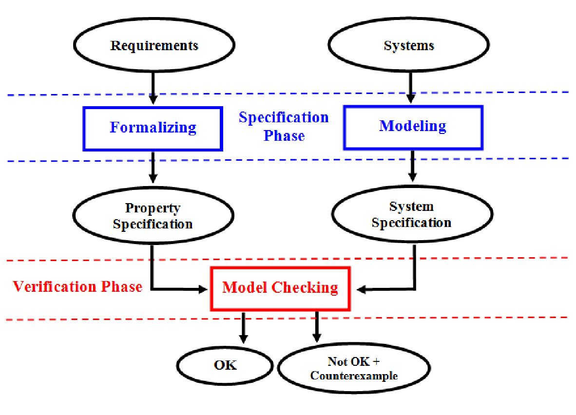
Usual properties that can be verified are “Can the system reach a deadlock state?”, or “Every sent message is received with probability at least 0.99?”. Such automated verification is carried on by a so-called model checker, an algorithm that exhaustively searches the space state of the model looking for states violating the (correctness) property.
A major strength of model checking is the capability of generating counterexamples which provide diagnostic information in case the property is violated. Edmund M. Clarke, one of the pioneers of Model Checking said [Cla08]: “It is impossible to overestimate the importance of the counterexample feature. The counterexamples are invaluable in debugging complex systems. Some people use model checking just for this feature”. In case a state violating the property under consideration is encountered, the model checker provides a counterexample describing a possible execution that leads from the initial state of the system to a violating state.
Other important advantages of model checking are: it is highly automatic so it requires little interaction and knowledge of designers, it is rather fast, it can be applied to a large range of problems, it allows partial specifications.
The main disadvantage of model checking is that the space state of certain systems, for instance distributed systems, can be rather large, thus making the verifications inefficient and in some cases even unfeasible (because of memory limitations). This problem is known as the state explosion problem. Many techniques to alleviate it have been proposed since the invention of model checking. Among the most popular ones we mention the use Binary Decision Diagrams (BDDs), partial order reduction, abstraction, compositional reasoning, and symmetry reduction. State-of-the-art model checkers can easily handle up to states with explicit state representation. For certain specific problems, more dedicated data structures (like BDDs) can be used thus making it possible to handle even up to states.
The popularity of model checking has grown considerably since its invention at the beginning of the 80s. Nowadays, model checking techniques are employed by most or all leading hardware companies (e.g. INTEL, IBM and MOTOROLA - just to mention few of them). While model checking is applied less frequently by software developing companies, there have been several cases in which it has helped to detect previously unknown defects in real-world software. A prominent example is the result of research in Microsoft’s SLAM project in which several formal techniques were used to automatically detect flaws in device drivers. In 2006, Microsoft released the Static Driver Verifier as part of Windows Vista, SDV uses the SLAM software-model-checking engine to detect cases in which device drivers linked to Vista violate one of a set of interface rules. Thus SDV helps uncover defects in device drivers, a primary source of software bugs in Microsoft applications. Investigations have shown that model checking procedures would have revealed the exposed defects in, e.g., Intel�s Pentium II processor and the Therac-25 therapy radiation machine.
Focus of this thesis
This thesis addresses the foundational aspects of formal methods for applications in security and in particular in anonymity: We investigate various issues that have arisen in the area of anonymity, we develop frameworks for the specification of anonymity properties, and we propose algorithms for their verification.
1.3 Background
In this section we give a brief overview of the various approaches to the foundations of anonymity that have been explored in the literature. We will focus on anonymity properties, although the concepts and techniques developed for anonymity apply to a large extent also to neighbor topics like information flow, secrecy, privacy. The common denominator of these problems is the prevention of the leakage of information. More precisely, we are concerned with situations in which there are certain values (data, identities, actions, etc) that are intended to be secret, and we want to ensure that an adversary will not be able to infer the secret values from the information which is publicly available. Some researchers use the term information hiding to refer to this class of problems [HO05].
The frameworks for reasoning about anonymity can be classified into two main categories: the possibilistic approaches, and the probabilistic (or quantitative) ones.
Possibilistic notions
The term “possibilistic” refers to the fact that we do not consider quantitative aspects. More precisely, anonymity is formulated in terms of the possibility or inferring some secrets, without worrying about “how likely” this is, or “how much” we narrow down the secret.
These approaches have been widely explored in the literature, using different conceptual frameworks. Examples include the proposals based on epistemic logic ([SS99, HO05]), on “function views” ([HS04]), and on process equivalences (see for instance [SS96, RS01]). In the following we will focus on the latter kind.
In general, possibilistic anonymity means that the observables do not identify a unique culprit. Often this property relies on nondeterminism: for each culprit, the system should be able to produce alternative executions with different observables, so that in turn for a given observable there are many agents that could be the culprit. More precisely, in its strongest version this property can be expressed as follows: if in one computation the identity of the culprit is and the observable outcome is , then for every other agent there must be a computation where, with culprit , the observable is still .
This kind of approach can be applied also in case of systems that use randomization. The way this is done is by abstracting the probabilistic choices into nondeterministic ones. See for example the Dining Cryptographers example in [SS96], where the coin tossing is represented by a nondeterministic process.
In general the possibilistic approaches have the advantages of simplicity an efficiency. On the negative side, they lack precision, and in some cases the approximation can be rather loose. This is because every scenario that has a non-null probability is interpreted as possible. For instance, consider the case in which a system reveals the culprit 90 percent of the times by outputting his identity, while in the remaining 10 percent of the times it outputs the name of some other agent. The system would not look very anonymous. Yet, the possibilistic definition of anonymity would be satisfied because all users would appear as possible culprits to the observer regardless of the output of the system. In general, in the possibilistic approach the strongest notion of anonymity we can express is possible innocence, which is satisfied when no agent appear to be the culprit for sure: there is always the possibility that he is innocent (no matter how unlikely it is).
In this thesis we consider only the probabilistic approaches. Their common feature is that they deal with probabilities in a concrete way and they are, therefore, much more precise. They have become very popular in recent times, and there has been a lot of work dedicated to understanding and formalizing the notion in a rigorous way. In the next section we give a brief overview of these efforts.
Probabilistic notions
These approaches take probabilities into account, and are based on the likelihood that an agent is the culprit, for a given observable. One notion of probabilistic anonymity which has been thoroughly investigated in the literature is strong anonymity.
Strong anonymity
Intuitively the idea behind this notion is that the observables should not allow to infer any (quantitative) information about the identity of the culprit. The corresponding notion in the field of information flow is (quantitative) non-interference.
Once we try to formalize more precisely the above notion we discover however that there are various possibilities. Correspondingly, there have been various proposals. We recall here the three most prominent ones.
- 1.
Equality of the a posteriori probabilities for different culprits. The idea is to consider a system strongly anonymous if, given an observable , the a posteriori probability that the identity of the culprit is , , is the same as the a posteriori probability of any other identity . Formally:
(1.1) This is the spirit of the definition of strong anonymity by Halpern and O’Neill [HO05], although their formalization involves more sophisticated epistemic notions.
- 2.
Equality of the a posteriori and a priori probabilities for the same culprit. Here the idea is to consider a system strongly anonymous if, for any observable, the a posteriori probability that the culprit is a certain agent is the same as its a priori probability. In other words, the observation does not increase or decrease the support for suspecting a certain agent. Formally:
(1.2) This is the definition of anonymity adopted by Chaum in [Cha88]. He also proved that the Dining Cryptographers satisfy this property if the coins are fair. Halpern and O’Neill consider a similar property in their epistemological setting, and they call it conditional anonymity [HO05].
- 3.
Equality of the likelihood of different culprits. In this third definition a system is strongly anonymous if, for any observable and agent , the likelihood of being the culprit, namely , is the same as the likelihood of any other agent . Formally:
(1.3) This was proposed as definition of strong anonymity by Bhargava and Palamidessi [BP05].
In [BCPP08] it has been proved that definitions (1.2) and (1.3) are equivalent. Definition (1.3) has the advantage that it does extend in a natural way to the case in which the choice of the culprit is nondeterministic. This could be useful when we do not know the a priori distribution of the culprit, or when we want to abstract from it (for instance because we are interested in the worst case).
Concerning Definition (1.1), it probably looks at first sight the most natural, but it actually turns out to be way too strong. In fact it is equivalent to (1.2) and (1.3), plus the following condition:
| (1.4) |
namely the condition that the a priori distribution be uniform.
It is interesting to notice that (1.1) can be split in two orthogonal properties: (1.3), which depends only in the protocol, and (1.4), which depends only in the distribution on the secrets.
Unfortunately all the strong anonymity properties discussed above are too strong, almost never achievable in practice. Hence researches have started exploring weaker notions. One of the most renowned properties of this kind (among the “simple” ones based on conditional probabilities) is that of probable innocence.
Probable innocence
The notion of probable innocence was formulated by Rubin and Reiter in the context of their work on the Crowds protocol [RR98]. Intuitively the idea is that, after the observation, no agent is more likely to be the culprit than not to be. Formally:
or equivalently
In [RR98] Rubin and Reiter proved that the Crowds protocol satisfies probable innocence under a certain assumption on the number of attackers relatively to the number of honest users.
All the notions discussed above are rather coarse, in the sense that they are cut-off notions and do not allow to represent small variations in the degree of anonymity. In order to be able to compare different protocols in a more precise way, researcher have started exploring settings to measure the degree of anonymity. The most popular of these approaches are those based in information theory.
Information theory
The underlying idea is that anonymity systems are interpreted as channels in the information-theoretic sense. The input values are the possible identities of the culprit, which, associated to a probability distribution, form a random variable . The outputs are the observables, and the transition matrix consists of the conditional probabilities of the form , representing the probability that the system produces an observable when the culprit is . A central notion here is the Shannon entropy, which represents the uncertainty of a random variable. For the culprit’s possible identity, this is given by:
Note that and the matrix also determine a probability distribution on the observables, which can then be seen as another random variable . The conditional entropy , representing the uncertainty about the identity of the culprit after the observation, is given by
It can be shown that . We have when there is no uncertainty left about after the value of is known. Namely, when the value of completely determines the value of . This is the case of maximum leakage. At the other extreme, we have when gives no information about , i.e. when and are independent.
The difference between and is called mutual information and it is denoted by :
The maximum mutual information between and over all possible input distributions is known as the channel’s capacity:
In the case of anonymity, the mutual information represents the difference between the a priori and the a posteriori uncertainties about the identity of the culprit. It can therefore be considered as the leakage of information due to the system, i.e. the amount of anonymity which is lost because of the observables produced by the system. Similarly, the capacity represents the worst-case leakage under all possible distributions on the culprit’s possible identities. It can be shown that the capacity is if and only if the rows of the matrix are pairwise identical. This corresponds exactly to the version (1.3) of strong anonymity.
This view of the degree of anonymity has been advocated in various works, including [MNCM03, MNS03, ZB05, CPP08a]. In the context of information flow, the same view of leakage in information theoretic terms has been widely investigated as well. Without pretending to be exhaustive, we mention [McL90, Gra91, CHM01, CHM05a, Low02, Bor06].
In [Smi09] Smith has investigated the use of an alternative notion of entropy, namely Rényi’s min entropy [Rén60], and has proposed to define leakage as the analogous of mutual information in the setting of Rényi’s min entropy. The justification for proposing this variant is that it represents better certain attacks called one-try attacks. In general, as Köpf and Basin illustrate in their cornerstone paper [KB07], one can use the above information-theoretic approach with many different notions of entropy, each representing a different model of attacker, and a different way of measuring the success of an attack.
A different information-theoretic approach to leakage has been proposed in [CMS09]: in that paper, the authors define as information leakage the difference between the a priori accuracy of the guess of the attacker, and the a posteriori one, after the attacker has made his observation. The accuracy of the guess is defined as the Kullback-Leibler distance between the belief (which is a weight attributed by the attacker to each input hypothesis) and the true distribution on the hypotheses. In [HSP10] a Rényi’s min entropy variant of this approach has been explored as well.
We conclude this section by remarking that, in all the approaches discussed above, the notion of conditional probability plays a central role.
1.4 Contribution and plan of the thesis
We have seen in Section 1.3 that conditional probabilities are the key ingredients of all quantitative definitions of anonymity. It is therefore desirable to develop techniques to analyze and compute such probabilities.
Our first contribution is cpCTL, a temporal logic allowing us to specify properties concerned with conditional probabilities in systems combining probabilistic and nondeterministic behavior. This is presented in Chapter 2. cpCTL is essentially pCTL (probabilistic Computational Tree Logic) [HJ94] enriched with formulas of the kind , stating that the probability of given is at most . We do so by enriching pCTL with formulas of the form . We propose a model checker for cpCTL. Its design has been quite challenging, due to the fact that the standard model checking algorithms for pCTL in MDPs (Markov Decision Processes) do not extend to conditional probability formulas. More precisely, in contrast to pCTL, verifying a conditional probability cannot be reduced to a linear optimization problem. A related point is that, in contrast to pCTL, the optimal probabilities are not attained by history independent schedulers. We attack the problem by proposing the notion of semi history independent schedulers, and we show that these schedulers do attain optimality with respect to the conditional probabilities. Surprisingly, it turns out that we can further restrict to deterministic schedulers, and still attain optimality. Based on these results, we show that it is decidable whether a cpCTL formula is satisfied in a MDP, and we provide an algorithm for it. In addition, we define the notion of counterexample for the logic and sketch an algorithm for counterexample generation.
Unfortunately, the verification of conditional cpCTL formulae is not efficient in the presence of nondeterminism. Another issue, related to nondeterminism within the applications in the field of security, is the well known problem of almighty schedulers (see Chapter 4). Such schedulers have the (unrealistic) ability to peek on internal secrets of the component and make their scheduling policy dependent on these secrets, thus leaking the secrets to external observers. We address these problems in separate chapters.
In Chapter 3 we restrict the framework to purely probabilistic models where secrets and observables do not interact, and we consider the problem of computing the leakage and the maximal leakage in the information-theoretic approach. These are defined as mutual information and capacity, respectively. We address these notions with respect to both the Shannon entropy and the Rényi min entropy. We provide techniques to compute channel matrices in time, where is the number of observables, and the number of states. (From the channel matrices, we can compute mutual information and capacity using standard techniques.) We also show that, contrarily to what was stated in literature, the standard information theoretical approaches to leakage do not extend to the case in which secrets and observable interact.
In Chapter 4 we consider the problem of the almighty schedulers. We define a restricted family of schedulers (admissible schedulers) which cannot base their decisions on secrets, thus providing more realistic notions of strong anonymity than arbitrary schedulers. We provide a framework to represent concurrent systems composed by purely probabilistic components. At the global level we still have nondeterminism, due to the various possible ways the component may interact with each other. Schedulers are then defined as devices that select at every point of the computation the component(s) moving next. Admissible schedulers make this choice independently from the values of the secrets. In addition, we provide a sufficient (but not necessary) technique based on automorphisms to prove strong anonymity for this family of schedulers.
The notion of counterexample has been approached indirectly in Chapters 2 and 3. In Chapter 5 we come back and fully focus on this topic. We propose a novel technique to generate counterexamples for model checking on Markov Chains. Our propose is to group together violating paths that are likely to provide similar debugging information thus alleviating the debugging tasks. We do so by using strongly connected component analysis and show that it is possible to extend these techniques to Markov Decision Processes.
Chapter 6 is an overview chapter. There we briefly describe extensions to the frameworks presented in Chapters 3 and 411 1 For more information about the topics discussed in this chapter we refer the reader to [AAP10a, AAP11, AAP10b, AAPvR10].. First, we consider the case in which secrets and observables interact, and show that it is still possible to define an information-theoretic notion of leakage, provided that we consider a more complex notion of channel, known in literature as channel with memory and feedback. Second, we extend the systems proposed in Chapter 4 by allowing nondeterminism also internally to the components. Correspondingly, we define a richer notion of admissible scheduler and we use it for defining notion of process equivalences relating to nondeterminism in a more flexible way than the standard ones in the literature. In particular, we use these equivalences for defining notions of anonymity robust with respect to implementation refinement.
In Figure 1.4 we describe the relation between the different chapters of the thesis. Chapter 5 is not explicitly depicted in the figure because it does not fit in any of the branches of cpCTL (efficiency - security foundations). However, the techniques developed in Chapter 5 have been applied to the works in both Chapters 2 and 3.

We conclude this thesis In Chapter 7, there we present a summary of our main contributions and discuss further directions.
1.5 Origins of the Chapters and Credits
In the following we list, for each chapter, the set of related articles together with their publication venue and corresponding co-authors.
-
Chapter 3 is based on the article [APvRS10a] by Catuscia Palamidessi, Peter van Rossum, Geoffrey Smith and myself. The article was presented in TACAS 2010.
-
Chapter 5 is based on the article [ADvR08] by Pedro D’Argenio, Peter van Rossum, and myself. The article was presented in HVC 2008.
-
Chapter 6 is based on
- –
The article [AAP10b] by Mário S. Alvim, Catuscia Palamidessi, and myself. This work was presented in LICS 2010 as part of an invited talk by Catuscia Palamidessi.
- –
The article [AAP10a] by Mário S. Alvim, Catuscia Palamidessi, and myself. This work presented in CONCUR 2010.
- –
The journal article [AAP11] by the same authors of the previous works.
- –
The article [AAPvR10] by Mário S. Alvim, Catuscia Palamidessi, Peter van Rossum, and myself. This work was presented in IFIP-TCS 2010.
- –
The chapters remain close to their published versions, thus there is inevitably some overlapping between them (in particular in their introductions where basic notions are explained).
A short note about authorship: I am the first author in all the articles and journal works included in this thesis with the exception of the ones presented in Chapter 6.
Chapter 2 Conditional Probabilities over Probabilistic and Nondeterministic Systems
In this chapter we introduce cpCTL, a logic which extends the probabilistic temporal logic pCTL with conditional probabilities allowing to express statements of the form “the probability of given is at most ”. We interpret cpCTL over Markov Chains and Markov Decision Processes. While model checking cpCTL over Markov Chains can be done with existing techniques, those techniques do not carry over to Markov Decision Processes. We study the class of schedulers that suffice to find the maximum and minimum conditional probabilities, show that the problem is decidable for Markov Decision Processes and propose a model checking algorithm. Finally, we present the notion of counterexamples for cpCTL model checking and provide a method for counterexample generation.
2.1 Introduction
Conditional probabilities are a fundamental concept in probability theory. In system validation these appear for instance in anonymity, risk assessment, and diagnosability. Typical examples here are: the probability that a certain message was sent by Alice, given that an intruder observes a certain traffic pattern; the probability that the dykes break, given that it rains heavily; the probability that component A has failed, given error message E.
In this chapter we introduce cpCTL (conditional probabilistic CTL), a logic which extends strictly the probabilistic temporal logic pCTL [HJ89] with new probabilistic operators of the form . Such formula means that the probability of given is at most . We interpret cpCTL formulas over Markov Chains (MCs) and Markov Decision Processes (MDPs). Model checking cpCTL over MCs can be done with model checking techniques for pCTL*, using the equality .
In the case of MDPs, cpCTL model checking is significantly more complex. Writing for the probability under scheduler , model checking reduces to computing . Thus, we have to maximize a non-linear function. (Note that in general .) Therefore, we cannot reuse the efficient techniques for pCTL model checking, since they heavily rely on linear optimization techniques [BdA95].
In particular we show that, differently from what happens in pCTL [BdA95], history independent schedulers are not sufficient for optimizing conditional reachability properties. This is because in cpCTL the optimizing schedulers are not determined by the local structure of the system. That is, the choices made by the scheduler in one branch may influence the optimal choices in other branches. We introduce the class of semi history-independent schedulers and show that these suffice to attain the optimal conditional probability. Moreover, deterministic schedulers still suffice to attain the optimal conditional probability. This is surprising since many non-linear optimization problems attain their optimal value in the interior of a convex polytope, which correspond to randomized schedulers in our setting.
Based on these properties, we present an (exponential) algorithm for checking whether a given system satisfies a formula in the logic. Furthermore, we define the notion of counterexamples for cpCTL model checking and provide a method for counterexample generation.
To the best of our knowledge, our proposal is the first temporal logic dealing with conditional probabilities.
Applications
Complex Systems.
One application of the techniques presented in this chapter is in the area of complex system behavior. We can model the probability distribution of natural events as probabilistic choices, and the operator choices as non-deterministic choices. The computation of maximum and minimum conditional probabilities can then help to optimize run-time behavior. For instance, suppose that the desired behavior of the system is expressed as a pCTL formula and that during run-time we are making an observation about the system, expressed as a pCTL formula . The techniques developed in this chapter allow us to compute the maximum probability of given and to identify the actions (non-deterministic choices) that have to be taken to achieve this probability.
Anonymizing Protocols.
Another application is in the area of anonymizing protocols. The purpose of these protocols is to hide the identity of the user performing a certain action. Such a user is usually called the culprit. Examples of these protocols are Onion Routing [CL05], Dining Cryptographers [Cha88], Crowds [RR98] and voting protocols [FOO92] (just to mention a few). Strong anonymity is commonly formulated [Cha88, BP05] in terms of conditional probability: A protocol is considered strongly anonymous if no information about the culprit’s identity can be inferred from the behavior of the system. Formally, this is expressed by saying that culprit’s identity and the observations, seen as random variables, are independent from each other. That is to say, for all users and all observations of the adversary :
P[culprit observation ] P[culprit ].
If considering a concurrent setting, it is customary to give the adversary full control over the network [DY83] and model its capabilities as nondeterministic choices in the system, while the user behavior and the random choices in the protocol are modeled as probabilistic choices. Since anonymity should be guaranteed for all possible attacks of the adversary, the above equality should hold for all schedulers. That is: the system is strongly anonymous if for all schedulers , all users and all adversarial observations :
Pη[culprit observation ] Pη[culprit ]
Since the techniques in this chapter allow us to compute the maximal and minimal conditional probabilities over all schedulers, we can use them to prove strong anonymity in presence of nondeterminism.
Similarly, probable innocence means that a user is not more likely to be innocent than not to be (where “innocent” mans “not the culprit”). In cpCTL this can be expressed as .
Organization of the chapter
In Section 2.2 we present the necessary background on MDPs. In Section 2.3 we introduce conditional probabilities over MDPs and in Section 2.4 we introduce cpCTL. Section 2.5 introduces the class of semi history-independent schedulers and Section 2.6 explains how to compute the maximum and minimum conditional probabilities. Finally, Section 2.7, we investigate the notion of counterexamples.
2.2 Markov Decision Processes
Markov Decision Processes constitute a formalism that combines nondeterministic and probabilistic choices. They are a dominant model in corporate finance, supply chain optimization, and system verification and optimization. While there are many slightly different variants of this formalism (e.g., action-labeled MDPs [Bel57, FV97], probabilistic automata [SL95, SdV04]), we work with the state-labeled MDPs from [BdA95].
The set of all discrete probability distributions on a set is denoted by . The Dirac distribution on an element is written as . We also fix a set of propositions.
Definition 2.2.1.
A Markov Decision Process (MDP) is a four-tuple where: is the finite state space of the system, is the initial state, is a labeling function that associates to each state a subset of propositions, and is a function that associates to each a non-empty and finite subset of of successor distributions.
In case for all states we say that is a Markov Chain.

We define the successor relation by and for each state we define the sets , and of paths and finite paths respectively beginning at . Sometimes we will use to denote , i.e. the set of paths of . For , we write the -th state of as . In addition, we write if is an extension of , i.e. for some . We define the basic cylinder of a finite path as the set of (infinite) paths that extend it, i.e . For a set of paths we write for its set of cylinders, i.e. . As usual, we let be the Borel -algebra on the basic cylinders.
Example 2.2.2. Figure 2.1 shows a MDP. States with double lines represent absorbing states (i.e., states with ) and is any constant in the interval . This MDP features a single nondeterministic decision, to be made in state .
Schedulers (also called strategies, adversaries, or policies) resolve the nondeterministic choices in a MDP [PZ93, Var85, BdA95].
Definition 2.2.3.
Let be a MDP and . An -scheduler for is a function from to such that for all we have . We denote the set of all -schedulers on by . When we omit it.
Note that our schedulers are randomized, i.e., in a finite path a scheduler chooses an element of probabilistically. Under a scheduler , the probability that the next state reached after the path is , equals . In this way, a scheduler induces a probability measure on defined as follows:
Definition 2.2.4.
Let be a MDP, , and an -scheduler on . The probability measure is the unique measure on such that for all
Often we will write instead of when is the initial state and . We now recall the notions of deterministic and history independent schedulers.
Definition 2.2.5.
Let be a MDP, , and an -scheduler for . We say that is deterministic if is either or for all and all . We say that a scheduler is history independent (HI) if for all finite paths of with we have .
Definition 2.2.6.
Let be a MDP, , and . Then the maximal and minimal probabilities of , , are defined as
A scheduler that attains or is called an optimizing scheduler.
We define the notion of (finite) convex combination of schedulers.
Definition 2.2.7.
Let be a MDP and let . An -scheduler is a convex combination of the -schedulers if there are with such that for all , .
Note that taking the convex combination of and as functions, i.e., , does not imply that is a convex combination of and in the sense above.
2.3 Conditional Probabilities over MDPs
The conditional probability is the probability of an event A, given the occurrence of another event B. Recall that given a probability space and two events with , is defined as If , then is undefined. In particular, given a MDP , a scheduler , and a state , consider the probabilistic space . For two sets of paths with , the conditional probability of given is If , then is undefined. We define the maximum and minimum conditional probabilities for all as follows:
Definition 2.3.1.
Let be a MDP. The maximal and minimal conditional probabilities , of sets of paths are defined by
where .
The following lemma generalizes Lemma 6 of [BdA95] to conditional probabilities.
Lemma 2.3.2.
Given , its maximal and minimal conditional probabilities are related by: .
2.4 Conditional Probabilistic Temporal Logic
The logic cpCTL extends pCTL with formulas of the form where . Intuitively, holds if the probability of given is at most . Similarly for the other comparison operators.
Syntax:
The cpCTL logic is defined as a set of state and path formulas, i.e., , where and are defined inductively:
Here and .
Semantics:
The satisfiability of state-formulas ( for a state ) and path-formulas ( for a path ) is defined as an extension of the satisfiability for pCTL. Hence, the satisfiability of the logical, temporal, and pCTL operators is defined in the usual way. For the conditional probabilistic operators we define
and similarly for and . We say that a model satisfy , denoted by if .
In the following we fix some notation that we will use in the rest of the chapter,
and are defined analogously.
Observation 2.4.1.
As usual, for checking if , we only need to consider the cases where and where is either or . This follows from , and the relations
derived from Lemma 2.3.2. Since there is no way to relate and , we have to provide algorithms to compute both and . The same remark holds for the minimal conditional probabilities and . In this chapter we will only focus on the former problem, i.e., computing maximum conditional probabilities, the minimal case follows using similar techniques.
2.4.1 Expressiveness
We now show that cpCTL is strictly more expressive than pCTL. The notion of expressiveness of a temporal logic is based on the notion of formula equivalence. Two temporal logic formulas and are equivalent with respect to a set of models (denoted by ) if for any model we have if and only if . A temporal logic is said to be at least as expressive as a temporal logic , over a set of models , if for any formula there is a formula that is equivalent to over . Two temporal logics are equally expressive when each of them is at least as expressive as the other. Formally:
Definition 2.4.1.
Two temporal logics and are equally expressive with respect to if
Theorem 2.4.2.
cpCTL is more expressive than pCTL with respect to MCs and MDPs.
Proof.
Obviously cpCTL is at least as expressive as pCTL, hence we only need to show that the reverse does not hold. The result is rather intuitive since the semantics of the conditional operator for cpCTL logic is provided by a non-linear equation whereas there is no pCTL formula with non-linear semantics.
The following is a formal proof. We plan to show that there is no pCTL formula equivalent to , with and atomic propositions. The proof is by cases on the structure of the pCTL formula . The most interesting case is when is of the form , so we will only prove this case. In addition we restrict our attention to ’s such that (the cases and are easy). In Figure 2.2 we depict the Markov Chains involved in the proof. We use to mark the states with an assignment of truth values (to propositional variables) falsifying .
- Case :
If is or the proof is obvious, so we assume otherwise. We first note that we either have or . In the former case, it is easy to see (using ) that we have and . In the second case we have and . - Case :
We assume , otherwise we fall into the previous case. We can easily see that we have but . - Case :
The case when is easy, so we assume . We can easily see that we have but .
∎
Note that, since MCs are a special case of MDPs, the proof also holds for the latter class.


We note that, in spite of the fact that a cpCTL formula of the form cannot be expressed as a pCTL formula, if dealing with fully probabilistic systems (i.e. systems without nondeterministic choices) it is still possible to verify such conditional probabilities formulas as the quotient of two pCTL formulas: . However, this observation does not carry over to systems where probabilistic choices are combined with nondeterministic ones (as it is the case of Markov Decision Processes). This is due to the fact that, in general, it is not the case that .
2.5 Semi History-Independent and Deterministic Schedulers
Recall that there exist optimizing (i.e. maximizing and minimizing) schedulers on pCTL that are and deterministic [BdA95]. We show that, for cpCTL, deterministic schedulers still suffice to reach the optimal conditional probabilities. Because we now have to solve a non-linear optimization problem, the proof differs from the pCTL case in an essential way. We also show that schedulers do not suffice to attain optimal conditional probability and introduce the family of semi history-independent schedulers that do attain it.
2.5.1 Semi History-Independent Schedulers
The following example shows that maximizing schedulers are not necessarily .

Example 2.5.1. Let be the MDP of Figure 2.3 and the conditional probability . There are only three deterministic history independent schedulers, choosing , , or in . For the first one, the conditional probability is undefined and for the second and third it is 0. The scheduler that maximizes satisfies , , and . Since chooses on first and later , is not history independent.
Fortunately, as we show in Theorem 2.5.3, there exists a nearly scheduler that attain optimal conditional probability. We say that such schedulers are nearly HI because they always take the same decision before the system reaches a certain condition and also always take the same decision after . This family of schedulers is called -semi history independent (- for short) and the condition is called stopping condition. For a pCTL path formula the stopping condition is a boolean proposition either validating or contradicting . So, the (validating) stopping condition of is whereas the (contradicting) stopping condition of is . Formally:
Similarly, for a cpCTL formula , the stopping condition is a condition either validating or contradicting any of its pCTL formulas (, ), i.e., .
We now proceed with the formalization of semi history independent schedulers.
Definition 2.5.2 (Semi History-Independent Schedulers).
Let be a MDP, a scheduler for , and . We say that is a semi history-independent scheduler (- scheduler for short) if for all such that we have
| {HI before stopping condition} | |||
| {HI after stopping condition} | |||
| {HI after stopping condition} |
We denote the set of all - schedulers of by .
We now prove that semi history-independent schedulers suffice to attain the optimal conditional probabilities for cpCTL formula.
Theorem 2.5.3.
Let be a MDP, , and . Assume that there exists a scheduler such that . Then:
(If there exists no scheduler such that , then the supremum is .)
The proof of this theorem is rather complex. The first step is to prove that there exists a scheduler HI before the stopping condition and such that is ‘close’ (i.e. not further than a small value ) to the optimal conditional probability . For this purpose we introduce some definitions and prove this property first for long paths (Lemma 2.5.5) and then, step-by-step, in general (Lemma 2.5.6 and Corollary 2.5.1). After that, we create a scheduler that is also HI after the stopping condition and whose conditional probability is still close to the optimal one (Lemma 2.5.7). From the above results, the theorem readily follows.
We now introduce some definitions and notation that we will need for the proof.
Definition 2.5.4 (Cuts).
Given a MDP we say that a set is a cut of if is a downward-closed set of finite paths such that every infinite path passes through it, i.e.
-
, and
-
where means that is an “extension” of , i.e. for some path . We denote the set of all cuts of by .
For , we say that is history independent in if for all such that we have that . We also define the sets and as the set of finite paths validating and respectively, i.e. and . Finally, given a MDP , two path formulas , , and we define the set
If a scheduler is HI in then we say that is HI before the stopping condition.
Lemma 2.5.5 (non emptiness of ).
There exists such that and that its complement is finite.
Proof.
We show that, given formulas , and , there exists a cut and a scheduler such that is finite, , is HI in , and .
The proof is by case analysis on the structure of and . We will consider the cases where and are either “eventually operators” () or “globally operators” (), the proof for the until case follows along the same lines.
Case is of the form and is of the form :
Let us start by defining the the probability of
reaching in at most steps, as . Note that for all pCTL reachability properties and schedulers we have
We also note that this result also holds for formulas of the form .
Let us now take a scheduler and a number such that
| (2.1) | ||||
| (2.2) | ||||
| (2.3) |
where is such that . The reasons for this particular choice for the bound of will become clear later on in the proof.
We define as , where the latter set is defined as the set of paths with length larger than , i.e. . In addition, we define as a scheduler HI in behaving like for paths of length less than or equal to which additionally minimizes after level . In order to formally define such a scheduler we let to be the set of states that can be reached in exactly steps, i.e., . Now for each we let to be a HI s-scheduler such that . Note that such a scheduler exists, i.e., it is always possible to find a HI scheduler minimizing a reachability pCTL formula [BdA95].
We now define as
where denotes the set of paths of of length . It is easy to see that minimizes after level . As for the history independency of in there is still one more technical detail to consider: note there may still be paths and such that and . This is the case when there is more than one distribution in minimizing , and happens to choose a different (minimizing) distribution than for the state . Thus, the selection of the family of schedulers must be made in such a way that: for all we have , , and for all . It is easy to check that such family exists. We conclude that is HI in and thus HI in .
Having defined we proceed to prove that such scheduler satisfies . It is possible to show that:
| (2.4) | ||||||||
| (2.5) |
(2.4) and the first inequality of (2.5) follow straightforwardly from the definition of . For the second inequality of (2.5) suppose by contradiction that . Then
contradicting (2.1).
Now we have all the necessary ingredients to show that
| (2.6) |
Note that
The first inequality holds because and (combining (2.5) and (2.2)) . The second inequality holds because and (combining (2.4) and (2.3)) . It is easy to see that falls in the same interval, i.e., both and are in the interval
Thus, we can prove (2.6) by proving
The first inequality holds if and only if . As for the second inequality, we have
We conclude, by definition of , that both inequalities hold.
Case is of the form and is of the form :
We now construct a cut and a scheduler
such that is finite, ,
is HI in , and
. Note that such a cut and
scheduler also satisfy .
The proof goes similarly to the previous case. We start by defining the probability of paths of length always satisfying as . Note that for all pCTL formula of the form and schedulers we have
The same result holds for the formula . It is easy to check that for all and we have .
Now we take a scheduler and a number such that:
where is such that .
We define as before, i.e., . In addition, we can construct (as we did in the previous case) a scheduler behaving as for paths of length at most and maximizing (instead of minimizing as in the previous case) afterwards. Again, it is easy to check that is HI in .
Then we have
In addition, it is easy to check that
Similarly to the previous case we now show that
| (2.7) |
which together with concludes the proof.
In order to prove (2.7) we show that
or, equivalently
- a)
, and
- b)
.
It is possible to verify that a) is equivalent to and that b) is equivalent to . The desired result follows by definition of . ∎
In the proof of the following lemma we step-by-step find pairs in with larger and still close to the optimal until finally is equal to the whole of .
Lemma 2.5.6 (completeness of ).
There exists a scheduler such that .
Proof.
We prove that if we take a such that is minimal then or, equivalently, . Note that a pair with minimal exists because, by the previous lemma, is not empty.
The proof is by contradiction: we suppose and arrive to a contradiction on the minimality of . Formally, we show that for all such that , there exists a cut and a scheduler such that , i.e. such that is HI in and .
To improve readability, we prove this result for the case is of the form and is of the form . However, all the technical details of the proof hold for arbitrary and .
Let us start defining the boundary of a cut as
Let be a path in such that . Note that by assumption of such exists. Now, if for all paths we have then is also HI in so we have as we wanted to show. Now let us assume otherwise, i.e. that there exists a path such that and . We let , , , and . Note that for all we have , this follows from the fact that is HI in .
Figure 2.4 provides a graphic representation of this description. The figure shows the set of all finite paths of , the cut of , the path reaching (in red and dotted border line style), a path reaching in (in blue and continuous border line style). The fact that takes different decisions and is represented by the different colors and line style of their respective last states .

We now define two schedulers and such that they are HI in . Both and are the same than everywhere but in and , respectively. The first one selects for all (instead of as does), and the second scheduler selects in (instead of ):
Now we plan to prove that either is “better” than or is “better” than . In order to prove this result, we will show that:
| (2.8) |
and
| (2.9) |
Therefore, if then we have , and otherwise . So, the desired result follows from (2.8) and (2.9). We will prove (2.8), the other case follows the same way.
In order to prove (2.8) we need to analyze more closely the conditional probability for each of the schedulers , and . For that purpose we partition the sets and into four parts, i.e. disjoint sets. The plan is to partition and in such way that we can make use of the fact that , , and are similar to each other (they only differ in the decision taken in or ) obtaining, in this way, that the probabilities of the parts are the same under these schedulers or differ only by a factor (this intuition will become clearer later on in the proof), such condition is the key element of our proof of (2.8). Let us start by partitioning :
- i)
We define as the set of paths in neither passing through nor , formally
- ii)
We define as the set of paths in passing through but not through , i.e.:
- iii)
We define as the set of paths in passing through and , i.e.:
- iv)
We define as the set of paths in passing through but not through , i.e.:
Note that
Similarly, we can partition the set of paths into four parts obtaining
In the following we analyze the probabilities (under ) of each part separately.
-
The probability of can be written as , where is the probability of and is the probability of reaching without passing through given . More formally,
-
The probability of can be written as , where is the probability of passing through given , is the probability of, given , reaching without passing through after ; and is the probability of, given , passing through again. Remember that is any path in . Formally, we have
Furthermore,
where .
-
The probability of can be written as , where is the probability of passing though without passing through . Formally,
-
Finally, we write the probability of as .
A similar reasoning can be used to analyze the probabilities associated to the parts of . In this way we obtain that (1) , where is the probability of reaching and without passing through given , (2) , where is the probability of reaching and without passing through afterwards given , (3) , and (4) .
In order to help the intuition of the reader, we now provide a graphical representation of the probability (under ) of the sets and by means of a Markov chain (see Figure 2.5). The missing values are defined as , ; and similarly for , , , and . Furthermore, absorbing states denote states where holds, absorbing states denote states where holds, and denote a state where holds. Finally, the state represents the state of the model where has been just reached and a state where any of the paths in as been just reached. To see how this Markov Chain is related to the probabilities of and on the original MDP consider, for example, the probabilities of the set . It is easy to show that
We note that the values , , , , and coincide for , , and . Whereas the values coincide for and and the values coincide for and . Thus, the variant of in which is replaced by describes the probability of each partition under the scheduler instead of . Similarly, the variant on which is replaced by represents the probability of each partition under the scheduler .
Now we have all the ingredients needed to prove (2.8). Our plan is to show that:
- 1)
, and
- 2)
where is the following determinant
We now proceed to prove 1)
A long but straightforward computation shows that the 2x2 determinant in the line above is equal to .
The proof of 2) proceeds along the same lines.
and also here a long computation shows that this last 2x2 determinant is equal to . ∎
Finally, we have all the ingredients needed to prove that there exists a scheduler close to the supremum which is HI before the stopping condition.
Corollary 2.5.1.
[HI before stopping condition] Let be a MDP, . Then for all , there exists a scheduler such that and is history independent before the stopping condition.
We now proceed with the construction of a maximizing scheduler and HI after the stopping condition.
Lemma 2.5.7.
[HI after stopping condition] Let be a MDP, , and . Then for all schedulers there exists a scheduler such that
- 1)
behaves like before the stopping condition,
- 2)
is HI after the stopping condition , and
- 3)
.
Proof.
We will prove this result for the case in which is of the form and is of the form , the proof for the remaining cases follows in the same way.
Let us start by introducing some notation. We define, respectively, the set of paths reaching , the set of paths not reaching , the set of paths reaching without reaching before, and the set of paths reaching without reaching before as follows
Note that the last two sets are disjoint. It is easy to check that
Let us now define the minimal set of finite paths “generating” (by their basic cylinders) and : and similarly . Note that and . Now we can write
The construction of the desired scheduler is in the spirit of the construction we proposed for the scheduler in Lemma 2.5.5. We let and . Note that and are disjoint. Now we define two families of schedulers and such that: for all we have , , and for all we have . Similarly for : for all we have , , and for all we have .
We now proceed to define :
where , and similarly .
It is easy to check that satisfies 1) and 2). As for 3) we first note that , , and .
In addition, we need the following simple remark.
Remark 2.5.8.
Let be a function defined as where and are constants in the interval such that . Then is increasing.
Finally, we have
2.5.2 Deterministic Schedulers
We now proceed to show that deterministic schedulers suffice to attain optimal conditional probabilities.
The following result states that taking the convex combination of schedulers does not increase the conditional probability .
Lemma 2.5.9.
Let be a MDP, a state, and path formulas. Suppose that the -scheduler is a convex combination of and . Then .
Proof.
To prove this lemma we need to use the following technical result: The function defined as below is monotonous.
where and . This claim follows from the fact that is always or always .
Now, by applying the result above to
we get that the maximum is reached at or . Because is a convex combination of and , (in the first case) or (in the second case). ∎
Lemma 2.5.10.
Let be a MDP, a state, and a path formula. Then every -sHI -scheduler on is a convex combination of deterministic -sHI -schedulers.
Proof.
The result follows from the fact that sHI schedulers have only finitely many choices to make at each state (at most two) and every choice at a particular state – either before or after the stopping condition– is a convex combination of deterministic choices at that state – either before or after the stopping condition. ∎
Finally, combining Theorem 2.5.3 and the previous lemma we obtain:
Theorem 2.5.11.
Let be a MDP, , and . Then we have
where is the set of deterministic and - schedulers of .
Since the number of deterministic and semi HI schedulers is finite we know that there exists a scheduler attaining the optimal conditional probability, i.e. . Note that this implies that cpCTL is decidable.
We conclude this section showing that there exists a deterministic and semi HI scheduler maximizing the conditional probabilities of Example 2.5.1.
Example 2.5.12.
Consider the MDP and cpCTL formula of Example 2.5.1. According to Theorem 2.5.11 there exists a deterministic and - scheduler that maximizes . In this case, a maximizing scheduler will take always the same decision () before the system reaches (a state satisfying the until stopping condition ) and always the same decision () after the system reaches .
2.6 Model Checking cpCTL
Model checking cpCTL means checking if a state satisfies a certain state formula . We focus on formulas of the form and show how to compute . The case is similar.
Recall that model checking pCTL is based on the Bellman-equations. For instance, whenever . So a scheduler that maximizes chooses maximizing . In a successor state , still behaves as a scheduler that maximizes . As shown below, such a local Bellman-equation is not true for conditional probabilities: a scheduler that maximizes a conditional probability such as does not necessarily maximize for successors of .
Example 2.6.1.
Consider the MDP and cpCTL formula of Figure 2.1. There are only two deterministic schedulers. The first one, , chooses when the system reaches the state and the second one, , chooses when the system reaches . For the first one , and for the second one . So . Therefore, if the scheduler that maximizes is () and otherwise it is ().
Furthermore, and ; the scheduler that obtains this last maximum is the one that chooses in .
Thus, if the scheduler that maximizes the conditional probability from is taking a different decision than the one that maximize the conditional probability from . Furthermore, for all , showing that the Bellman-equation from above does not generalize to cpCTL.
As consequence of this observation, it is not possible to “locally maximize” cpCTL properties (i.e. to obtain the global maximum by maximizing for all states ). This has a significant impact in terms of model-checking complexity: as we will show in the rest of this section, to verify a cpCTL property it is necessary to compute and keep track of several conditional probabilities and the desired maximum value can only be obtained after all these probabilities have been collected.
2.6.1 Model Checking
An obvious way to compute is by computing the pairs (, ) for all deterministic schedulers , and then taking the maximum quotient . This follows from the fact that there exist finitely many deterministic semi history-independent schedulers and that one of them attains the maximal conditional probability; however, the number of such schedulers grows exponentially in the size of the MDP so computing these pairs for all of them is computationally expensive. Our plan is to first present the necessary techniques to naively compute (, ) for all deterministic schedulers and then present an algorithm that allows model checking without collecting such pairs for all scheduler.
1) A naive approach to compute
The algorithm is going to keep track of a list of pairs of probabilities of the form (, ) for all states and a deterministic scheduler. We start by defining a data structure to keep track of the these pairs of probabilities.
Definition 2.6.2.
Let be the set of expressions of the form where and , for all . On we consider the smallest congruence relation satisfying idempotence, commutativity, and associativity, i.e.:
Note that if and only if .
We let be the set of equivalence classes and denote the projection map that maps each expression to its equivalence class by . On we also define maximum quotient by
Note that induces a map making the diagram in Figure 2.6(b) (a) commute, i.e., such that .
Definition 2.6.3.
Let be a MDP. We define the function by
and we define by .


When no confusion arises, we omit the subscripts 1 and omit the projection map , writing for the equivalence class it generates.
Example 2.6.4. In Figure 2.6(b) we show the value associated to each state of the MDP in Figure 2.1.
The following lemma states that it is possible to obtain maximum conditional probabilities using .
Lemma 2.6.5.
Given an acyclic MDP, and . Then
and
where and .
Proof.
The lemma follows straightforwardly from the definitions of and and the fact that the maximum conditional probability is indeed reached by a deterministic scheduler. ∎
Remember that there are finitely many schedulers. Thus, (and therefore ) can in principle be computed by explicitly listing them all. However, this is of course an inefficient way to compute maximum conditional probabilities.
We now show how to compute in a more efficient way. We will first provide an algorithm to compute maximum conditional probabilities for acyclic MDPs. We then show how to apply this algorithm to MDPs with cycles by mean of a technique, based on SCC analysis, that allows the transformation of an MDP with cycles to an equivalent acyclic MDP.
2) An algorithm to compute for Acyclic MDPs
We will now present a recursive algorithm to compute for acyclic MDPs using a variant of (changing its image). As we mentioned before, to compute maximum conditional probabilities it is not necessary to consider all the pairs (with a deterministic and semi HI scheduler). In particular, we will show that it is sufficient to consider only deterministic and semi HI schedulers (see definition of below) that behave as an optimizing scheduler (i.e. either maximizing or minimizing a pCTL formula ) after reaching the stopping condition (i.e. a state satisfying ).
We plan to compute a function such that . Intuitively, can be thought as
where contains all deterministic and semi HI schedulers such that optimizes for some and formula.
This intuition will become evident when we present our recursive algorithm to compute conditional probabilities (see Theorem 2.6.11 below). The states involved in the definition of correspond to the base case of the algorithm and the formula corresponds to the formula that the algorithm maximizes/minimizes when such is reached.
We will present algorithms to recursively (in ) compute and in acyclic MDPs. The base cases of the recursion are the states where the stopping condition holds. In the recursive case we can express (respectively ) in terms of the (respectively ) of the successors states of .
We start by formalizing the notion of acyclic MDP. We call a MDP acyclic if it contains no cycles other than the trivial ones (i.e., other than selfloops associated to absorbing states).
Definition 2.6.6.
A MDP is called acyclic if for all states and all we have or , and, furthermore, for all paths , if there exist such that and , then we have for all .
In addition, in order to formally define we define a new congruence .
Definition 2.6.7.
Consider the set of expressions defined in Definition 2.6.2. On we now consider the smallest congruence relation containing and satisfying
- (1)
, and
- (2)
, and
- (3)
,
where . We write for the set of equivalence classes and denote the projection map by .
Since , this projection maps factors through , say is the unique map such that
Definition 2.6.8.
We define by .
Now, in order to prove that we need to define a scalar multiplication operator and an addition operator on .
Definition 2.6.9.
We define and by
Note that and induce maps and as shown in Figure 2.6 below. As before, we omit the subscript 1 if that will not cause confusion.


The following seemingly innocent lemma is readily proven, but it contains the key to allow us to discard certain pairs of probabilities. The fact that induces operations on means that it is correct to “simplify” expressions using when we are interested in the maximum or minimum quotient.
The intuition is as follows. Normally, which decision is best in a certain state (or rather, at a certain finite path) to optimize the conditional probability, might depend on probabilities or choices in a totally different part of the automaton (see Example 2.6.1). Sometimes, however, it is possible to decide locally what decision the scheduler should take. The congruence encodes three such cases, each of them corresponding to one clause in Definition 2.6.7. (1) If from a state the scheduler can either take a transition after which and or a transition after which and , then in order to maximize the conditional probability is always best to take the decision where . (2) Similarly, if the scheduler can either take a transition after which and or one after which and , then it is always best to take the decision where . (3) Finally, if has the option to either take a transition after which and or one after which and , for some , then a maximizing scheduler should always take the first of these two options.
Lemma 2.6.10.
The operators , and on induce operators , and on .
Proof.
The idempotence, commutativity and associativity cases are trivial; we only treat the other three cases.
- ( )
For (1) we have
Additionally, note that since and we have .
For (2) the proof goes like in (1). For (3) we have the following
- ( )
For (1) we have
For (2) the proof goes like in (1). For (3) we have the following
- ( )
For (1) we will start by assuming that . Then
Now assume that and the case is similar. Note that we now have that . Then
Finally, assume that , then also , so
For (2) the proof goes like in (1). For (3) we first need the following.
Let be a function defined as where and are constants in the interval . Then is increasing. Let us now assume that or . Then
Now assume that . Then
∎
The fact that follows from previous lemma.
Finally, the following theorem provides recursive equations for the values of and . If the MDPs is acyclic, it can be used to compute these values.
Theorem 2.6.11.
Let be a MDP, , and . Then
and
Proof.
We will consider the case . We will use to denote , i.e., the stopping condition of cpCTL formula under consideration.
- (a)
Note that if , then semi HI schedulers are exactly the HI schedulers, i.e., .
- (b)
- (c)
- (d)
- (e)
From MDPs to Acyclic MDPs
Now, we show how to reduce a MDP with cycles to an acyclic one, thus generalizing our results to MDPs with cycles. For that purpose we first reduce all cycles in and create a new acyclic MDP such that the probabilities involved in the computation of are preserved. We do so by removing every strongly connected component () of (the graph of) , keeping only input states and transitions to output states (in the spirit of [ADvR08]). We show that on is equal to the corresponding value on . For this, we have to make sure that states satisfying the stopping condition are ignored when removing s.
(1) Identifying s.
Our first step is to make states satisfying the stopping condition absorbing.
Definition 2.6.12.
Let be a MDP and a state formula. We define a new MDP where is equal to if and to otherwise.
To recognize cycles in the MDP we define a graph associated to it.
Definition 2.6.13.
Let be MDP and . We define the digraph associated to where satisfies .
![[Uncaptioned image]](1111.2760v1/InOutStates.png)
Now we let be the set of of . For each we define the sets of all states in that have an incoming transition of from a state outside of ; we also define the set of all states outside of that have an incoming transition from a state of . Formally, for each we define
where is the successor relation defined in Section 2.2.
We then associate a MDP to each of . The space of states of is and the transition relation is induced by the transition relation of .
Definition 2.6.14.
Let be a MDP and be a SCC in . We pick an arbitrary element of and define the MDP where and is equal to if and to otherwise.
(2) Constructing an acyclic MDP.
To obtain a reduced acyclic MDP from the original one we first define the probability of reaching one state from another according to a given scheduler in the following way.
Definition 2.6.15.
Let be a MDP, and be a scheduler on . Then for each we define the function such that .
We note that such reachability values can be efficiently computed using steady-state analysis techniques [Cas93].
Now we are able to define an acyclic MDP related to such that .
Definition 2.6.16.
Let be a MDP. Then we define as where
and for all the set of probabilistic distributions on is given by
Here is the associated to .
Theorem 2.6.17.
Let be a MDP, and . Then is an acyclic MDP and where represents on the MDP .
Proof.
The proof follows straightforwardly by the construction of and Theorem 2.5.11.∎
Finally we can use the technique for acyclic MDPs on the reduced MDP in order to obtain .
2.6.2 Complexity
As mentioned before, when computing maximum or minimum conditional probabilities it is not possible to locally optimize. Therefore, it is necessary to carry on, for each deterministic and HI scheduler , the pair of probabilities from the leafs (states satisfying the stopping condition) to the initial state. As the number of HI schedulers in a MDP grows exponentially on the state space, our algorithm to verify cpCTL formulas has exponential time complexity.
We believe that the complexity of computing optimal conditional probabilities is intrinsically exponential, i.e. computing such probabilities is an NP problem. However, a deeper study on this direction is still missing,
Conditional probability bounds
Even if computing exact conditional probabilities is computationally expensive (exponential time), it is still possible to efficiently compute upper and lower bounds for such probabilities (polynomial time).
Observation 2.6.1.
Let be a MDP and two path pCTL formulas. Then we have
2.7 Counterexamples for cpCTL
Counterexamples in model checking provide important diagnostic information used, among others, for debugging, abstraction-refinement [CGJ+00], and scheduler synthesis [LBB+01]. For systems without probability, a counterexample typically consists of a path violating the property under consideration. Counterexamples in MCs are sets of paths. E.g, a counterexample for the formula is a set of paths, none satisfying , and such that the probability mass of is greater than [HK07a, ADvR08, AL06].
In MDPs, we first have to find the scheduler achieving the optimal probability. Both for pCTL and cpCTL, this scheduler can be derived from the algorithms computing the optimal probabilities [ADvR08]. Once the optimal scheduler is fixed, the MDP can be turned into a Markov Chain and the approaches mentioned before can be used to construct counterexamples for pCTL. For cpCTL however, the situation is slightly more complex. It follows directly from the semantics that:
Lemma 2.7.1.
Let and consider the formula . Let , , and . Then implies .
Proof.
We first note that
Then, it is easy to see that
This leads to the following notion of counterexample.
Definition 2.7.2.
A counterexample for is a pair of measurable sets of paths satisfying , , and , for some scheduler .
Note that such sets and can be computed using the techniques on Markov Chains mentioned above.
Example 2.7.3. Consider the evaluation of on the MDP obtained by taking in the MDP depictured in Figure 2.1. The corresponding MDP is shown in Figure 2.7(a). In this case the maximizing scheduler, say , chooses in . In Figure 2.7(b) we show the Markov Chain derived from MDP using . In this setting we have and consequently does not satisfy this formula.


Chapter 3 Computing the Leakage of Information Hiding Systems
In this chapter we address the problem of computing the information leakage of a system in an efficient way. We propose two methods: one based on reducing the problem to reachability, and the other based on techniques from quantitative counterexample generation. The second approach can be used either for exact or approximate computation, and provides feedback for debugging. These methods can be applied also in the case in which the input distribution is unknown. We then consider the interactive case and we point out that the definition of associated channel proposed in literature is not sound. We show however that the leakage can still be defined consistently, and that our methods extend smoothly.
3.1 Introduction
By information hiding, we refer generally to the problem of constructing protocols or programs that protect sensitive information from being deduced by some adversary. In anonymity protocols [CPP08a], for example, the concern is to design mechanisms to prevent an observer of network traffic from deducing who is communicating. In secure information flow [SM03], the concern is to prevent programs from leaking their secret input to an observer of their public output. Such leakage could be accidental or malicious.
Recently, there has been particular interest in approaching these issues quantitatively, using concepts of information theory. See for example [MNCM03, CHM05b, DPW06, CMS09, CPP08a]. The secret input and the observable output of an information-hiding system are modeled as random variables related by a channel matrix, whose entry specifies , the conditional probability of observing output given input . If we define the vulnerability of as the probability that the adversary could correctly guess the value of in one try, then it is natural to measure the information leakage by comparing the a priori vulnerability of with the a posteriori vulnerability of after observing . We consider two measures of leakage: additive, which is the difference between the a posteriori and a priori vulnerabilities; and multiplicative, which is their quotient [Smi09, BCP09].
We thus view a protocol or program as a noisy channel, and we calculate the leakage from the channel matrix and the a priori distribution on . But, given an operational specification of a protocol or program, how do we calculate the parameters of the noisy channel: the sets of inputs and outputs, the a priori distribution, the channel matrix, and the associated leakage? These are the main questions we address in this chapter. We focus on probabilistic automata, whose transitions are labeled with probabilities and actions, each of which is classified as secret, observable, or internal.
We first consider the simple case in which the secret inputs take place at the beginning of runs, and their probability is fixed. The interpretation in terms of noisy channel of this kind of systems is well understood in literature. The framework of probabilistic automata, however, allows to represent more general situations. Thanks to the nondeterministic choice, indeed, we can model the case in which the input distribution is unknown, or variable. We show that the definition of channel matrix extends smoothly also to this case. Finally, we turn our attention to the interactive scenario in which inputs can occur again after outputs. This case has also been considered in literature, and there has been an attempt to define the channel matrix in terms of the probabilities of traces [DJGP02]. However it turns out that the notion of channel is unsound. Fortunately the leakage is still well defined, and it can be obtained in the same way as the simple case.
We consider two different approaches to computing the channel matrix. One uses a system of linear equations as in reachability computations. With this system of equations one can compute the joint matrix, the matrix of probabilities of observing both and ; the channel matrix is trivially derived from this joint matrix. The other approach starts with a channel matrix, which we call a partial matrix at this point. We iteratively add the contributions in conditional probabilities of complete paths to this partial matrix, obtaining, in the limit, the channel matrix itself. We then group paths with the same secret and the same observable together using ideas from quantitative counterexample generation, namely by using regular expressions and strongly connected component analysis. In this way, we can add the contribution of (infinitely) many paths at the same time to the partial matrices. This second approach also makes it possible to identify which parts of a protocol contribute most to the leakage, which is useful for debugging.
Looking ahead, after reviewing some preliminaries (Section 3.2) we present restrictions on probabilistic automata to ensure that they have well-defined and finite channel matrices (Section 3.3). This is followed by the techniques to calculate the channel matrix efficiently (Section 3.4 and Section 3.5). We then turn our attention to extensions of our information-hiding system model. We use nondeterministic choice to model the situation where the a priori distribution on the secret is unknown (Section 3.6). Finally, we consider interactive systems, in which secret actions and observable actions can be interleaved arbitrarily (Section 3.7).
3.2 Preliminaries
3.2.1 Probabilistic automata
This section recalls some basic notions on probabilistic automata. More details can be found in [Seg95]. A function is a discrete probability distribution on a set if the support of is countable and . The set of all discrete probability distributions on is denoted by .
A probabilistic automaton is a quadruple where is a countable set of states, a finite set of actions, the initial state, and a transition function . Here is the set of all finite subsets of . If then is a terminal state. We write for . Moreover, we write for whenever and . A fully probabilistic automaton is a probabilistic automaton satisfying for all states. In case we will overload notation and use to denote the distribution outgoing from .
A path in a probabilistic automaton is a sequence where , and . A path can be finite in which case it ends with a state. A path is complete if it is either infinite or finite ending in a terminal state. Given a path , denotes its first state, and if is finite then denotes its last state. A cycle is a path such that . We denote the set of actions occurring in a cycle as . Let denote the set of all paths, the set of all finite paths, and the set of all complete paths of an automaton , starting from the state . We will omit if . Paths are ordered by the prefix relation, which we denote by . The trace of a path is the sequence of actions in obtained by removing the states, hence for the above we have . If , then is the projection of on the elements of . The length of a finite path , denoted by , is the number of actions in its trace.
Let be a (fully) probabilistic automaton, a state, and let be a finite path starting in . The cone generated by is the set of complete paths Given a fully probabilistic automaton and a state , we can calculate the probability value, denoted by , of any finite path starting in as follows: and .
Let be the sample space, and let be the smallest -algebra generated by the cones. Then induces a unique probability measure on (which we will also denote by ) such that for every finite path starting in . For we write instead of .
Given a probability space and two events with , the conditional probability of given , , is defined as
3.2.2 Noisy Channels
This section briefly recalls the notion of noisy channels from Information Theory [CT06].
A noisy channel is a tuple where is a finite set of input values, modeling the secrets of the channel, and is a finite set of output values, the observables of the channel. For and , is the conditional probability of obtaining the output given that the input is . These conditional probabilities constitute the so called channel matrix, where is the element at the intersection of the -th row and the -th column. For any input distribution on , and the channel matrix determine a joint probability on , and the corresponding marginal probability on (and hence a random variable ). is also called a priori distribution and it is often denoted by . The probability of the input given the output is called a posteriori distribution.
3.2.3 Information leakage
We recall now some notions of information leakage which allow us to quantify the probability of success of a one-try attacker, i.e. an attacker that tries to obtain the value of the secret in just one guess. In particular, we consider Smith’s definition of multiplicative leakage [Smi09]11 1 The notion proposed by Smith in [Smi09] was given in a (equivalent) logarithmic form, and called simply leakage. For uniformity’s sake we use here the terminology and formulation of [BCP09]., and the additive leakage definition from Braun et al. [BCP09]. We assume given a noisy channel and a random variable on . The a priori vulnerability of the secrets in is the probability of guessing the right secret, defined as The rationale behind this definition is that the adversary’s best bet is on the secret with highest probability.
The a posteriori vulnerability of the secrets in is the probability of guessing the right secret, after the output has been observed, averaged over the probabilities of the observables. The formal definition is Again, this definition is based on the principle that the adversary will choose the secret with the highest a posteriori probability.
Note that, using Bayes theorem, we can write the a posteriori vulnerability in terms of the channel matrix and the a priori distribution, or in terms of the joint probability:
| (3.1) |
The multiplicative leakage is then defined as the quotient between the a posteriori and a priori vulnerabilities, . Similarly, the additive leakage is defined as the difference between both vulnerabilities, .
3.3 Information Hiding Systems
To formally analyze the information-hiding properties of protocols and programs, we propose to model them as a particular kind of probabilistic automata, which we call Information-Hiding Systems (IHS). Intuitively, an IHS is a probabilistic automaton in which the actions are divided in three (disjoint) categories: those which are supposed to remain secret (to an external observer), those which are visible, and those which are internal to the protocol.
First we consider only the case in which the choice of the secret takes place entirely at the beginning, and is based on a known distribution. Furthermore we focus on fully probabilistic automata. Later in the chapter we will relax these constraints.
Definition 3.3.1 (Information-Hiding System).
An information-hiding system (IHS) is a quadruple where is a fully probabilistic automaton, where , , and are pairwise disjoint sets of secret, observable, and internal actions, and satisfies the following restrictions:
- 1.
,
- 2.
- 3.
for ,
- 4.
,
- 5.
.
The first two restrictions are on the initial state and mean that only secret actions can happen there () and each of those actions must have non null probability and occur only once (), Restriction forbids secret actions to happen in the rest of the automaton, and Restriction specifies that only internal actions can occur inside cycles, this restriction is necessary in order to make sure that the channel associated to the IHS has finitely many inputs and outputs. Finally, Restriction means that infinite computations have probability and therefore we can ignore them.
We now show how to interpret an IHS as a noisy channel. We call and the secret and observable traces of , respectively. For , we define ; similarly for , we define .
Definition 3.3.2.
Given an IHS , its noisy channel is , where , , and . The a priori distribution of is defined by . If is the noisy channel of , the multiplicative and additive leakage of are naturally defined as
Example 3.3.3. Crowds [RR98] is a well-known anonymity protocol, in which a user (called the initiator) wants to send a message to a

web server without revealing his identity. To achieve this, he routes the message through a crowd of users participating in the protocol. Routing is as follows. In the beginning, the initiator randomly selects a user (called a forwarder), possibly himself, and forwards the request to him. A forwarder performs a probabilistic choice. With probability (a parameter of the protocol) he selects a new user and again forwards the message. With probability he sends the message directly to the server. One or more users can be corrupted and collaborate with each other to try to find the identity of the initiator.
We now show how to model Crowds as an for honest and corrupted user. We assume that the corrupted user immediately forwards messages to the server, as there is no further information to be gained for him by bouncing the message back.
Figure 3.1 shows the automaton22 2 For the sake of simplicity, we allow the initiator of the protocol to send the message to the server also in the first step of the protocol.. Actions and are secret and represent who initiates the protocol; actions , , and are observable; and represent who forwards the message to the corrupted user; represents the fact that the message arrives at the server undetected by the corrupted user. We assume to be observable to represent the possibility that the message is made publically available at the server’s site.
The channel associated to this IHS has , , and a priori distribution . Its channel matrix is computed in the next section.
3.4 Reachability analysis approach
This section presents a method to compute the matrix of joint probabilities associated to an , defined as
We omit the subscript when no confusion arises. From we can derive the channel matrix by dividing by . The leakage can be computed directly from , using the second form of the a posteriori vulnerability in (4.2.3).
We write for the probability of the set of paths with trace starting from the state of :
where . The following key lemma shows the linear relation between the ’s. We assume, w.l.o.g., that the has a unique final state .
Lemma 3.4.1.
Let be an . For all and we have
Furthermore, for and we have .
Using this lemma, one can compute joint probabilities by solving the system of linear equations in the variables ’s. It is possible that the system has multiple solutions; in that case the required solution is the minimal one.
Example 3.4.2.
Continuing with the Crowds example, we show how to compute joint probabilities. Note that . The linear equations from Lemma 3.4.1 are
Let us fix . By solving the system of linear equations we obtain
We can now compute the channel matrix by dividing each by . The result is shown in the figure above.
3.4.1 Complexity Analysis
We now analyze the computational complexity for the computation of the channel matrix of a simple . Note that the only variables (from the system of equations in Lemma 3.4.1) that are relevant for the computation of the channel matrix are those for which it is possible to get the trace starting from state . As a rough overestimate, for each state , there are at most ’s possible: in the initial state one can have every secret and every observable, in the other states no secret is possible and only a suffix of an observable can occur. This gives at most variables. Therefore, we can straightforwardly obtain the desired set of values in time (using Gaussian Elimination). Note that using Strassen’s methods the exponent reduces to , this consideration applies to similar results in the rest of the chapter as well.
Because secret actions can happen only at the beginning, the system of equations has a special form. The variables of the form only depend on variables of the form (with varying and ) and not on each other. Hence, we can first solve for all variables of the form and then compute the remaining few of the form . Required time for the first step is and the time for the second step can be ignored.
Finally, in some cases not only do the secret actions happen only at the beginning of the protocol, but the observable actions happen only at the end of the protocol, i.e., after taking a transition with an observable action, the protocol only performs internal actions (this is, for instance, the case for our model of Crowds). In this case, one might as well enter a unique terminal state after an observable action happens. Then the only relevant variables are of the form , , and ; the only depends on the , the only depend on (with the same , but varying ’s) and on and . Again ignoring the variables for complexity purposes, the system of equations has a block form with blocks of (at most) variables each. Hence the complexity in this case decreases to .
3.5 The Iterative Approach
We now propose a different approach to compute channel matrices and leakage. The idea is to iteratively construct the channel matrix of a system by adding probabilities of sets of paths containing paths with the same observable trace and secret trace to the entry of the matrix.
One reason for this approach is that it allows us to borrow techniques from quantitative counterexample generation. This includes the possibility of using or extending counterexample generation tools to compute channel matrices or leakage. Another reason for this approach is the relationship with debugging. If a (specification of a) system has a high leakage, the iterative approach allows us to determine which parts of the system contribute most to the high leakage, possibly pointing out flaws of the protocol. Finally, if the system under consideration is very large, the iterative approach allows us to only approximate the leakage (by not considering all paths, but only the most relevant ones) under strict guarantees about the accuracy of the approximation. We will focus on the multiplicative leakage; similar results can be obtained for the additive case.
3.5.1 Partial matrices
We start by defining a sequence of matrices converging to the channel matrix by adding the probability of complete paths one by one. We also define partial version of the a posteriori vulnerability and the leakage. Later, we show how to use techniques from quantitative counterexample generation to add probabilities of many (maybe infinitely many) complete paths all at once.
Definition 3.5.1.
Let be an , its a priori distribution, and an enumeration of the set of complete paths of . We define the partial matrices as follows
We define the partial vulnerability as , and the partial multiplicative leakage as .
The following lemma states that partial matrices, a posteriori vulnerability, and leakage converge to the correct values.
Lemma 3.5.2.
Let be an . Then
- 1.
, and
- 2.
, and ,
- 3.
, and .
Since rows must sum up to , this technique allow us to compute matrices up to given error . We now show how to estimate the error in the approximation of the multiplicative leakage.
Proposition 3.5.1.
Let be an . Then we have
where denotes the mass probability of the -th row of , i.e. .
3.5.2 On the computation of partial matrices.
After showing how partial matrices can be used to approximate channel matrices and leakage we now turn our attention to accelerating the convergence. Adding most likely paths first is an obvious way to increase the convergence rate. However, since automata with cycles have infinitely many paths, this (still) gives an infinite amount of path to process. Processing many paths at once (all having the same observable and secret trace) tackles both issues at the same time: it increases the rate of convergence and can deal with infinitely many paths at the same time,
Interestingly enough, these issues also appear in quantitative counterexample generation. In that area, several techniques have already been provided to meet the challenges; we show how to apply those techniques in the current context. We consider two techniques: one is to group paths together using regular expressions, the other is to group paths together using strongly connected component analysis.
Regular expressions.
In [Daw05], regular expressions containing probability values are used to reason about traces in Markov Chains. This idea is used in [DHK08] in the context of counterexample generation to group together paths with the same observable behaviour. The regular expression there are over pairs with a probability value and a state, to be able to track both probabilities and observables. We now use the same idea to group together paths with the same secret action and the same observable actions.
We consider regular expressions over triples of the form with a probability value, an action label and a state. Regular expressions represent sets of paths as in [DHK08]. We also take the probability value of such a regular expression from that article.
Definition 3.5.3.
The function evaluates regular expressions:
The idea is to obtain regular expressions representing sets of paths of , each regular expression will contribute in the approximation of the channel matrix and leakage. Several algorithms to translate automata into regular expressions have been proposed (see [Neu05]). Finally, each term of the regular expression obtained can be processed separately by adding the corresponding probabilities [Daw05] to the partial matrix.
As mentioned before, all paths represented by the regular expression should have the same observable and secret trace in order to be able to add its probability to a single element of the matrix. To ensure that condition we request the regular expression to be normal, i.e., of the form with the containing no ’s.
We will now describe this approach by an example.
Example 3.5.4.
where . We also note
where the symbols between brackets denote the secret and observable traces of each regular expression.
Now we have all the ingredients needed to define partial matrices using regular expressions.
Definition 3.5.5.
Let be an , its a priori distribution, and a regular expression equivalent to in normal form. We define for the matrices as follows
Note that in the context of Definition 3.5.5, we have .
SCC analysis approach.
In [ADvR08], paths that only differ in the way they traverse strongly connected components (’s) are grouped together. Note that in our case, such paths have the same secret and observable trace since secret and observable actions cannot occur on cycles. Following [ADvR08], we first abstract away the ’s, leaving only probabilistic transitions that go immediately from an entry point of the SCC to an exit point (called input and output states in [ADvR08]). This abstraction happens in such a way that the observable behaviour of the automaton does not change.
Instead of going into technical details (which also involves translating the work [ADvR08] from Markov Chains to fully probabilistic automata), we describe the technique by an example.

Example 3.5.6.
Figure 3.2 shows the automaton obtained after abstracting . In the following we show the set of complete paths of the automaton, together with their corresponding probabilities and traces
Note that the analysis approach groups more paths together (for instance group together the same paths than the regular expressions and in the examples of this section), as a result channel matrix and leakage are obtained faster. On the other hand, regular expressions are more informative providing more precise feedback.
3.5.3 Identifying high-leakage sources
We now describe how to use the techniques presented in this section to identify sources of high leakage of the system. Remember that the a posteriori vulnerability can be expressed in terms of joint probabilities
This suggests that, in case we want to identify parts of the system generating high leakage, we should look at the sets of paths where and . In fact, the multiplicative leakage is given dividing by , but since is a constant value (i.e., it does not depend on the row) it does not play a role here. Similarly for the additive case.
The techniques presented in this section allow us to obtain such sets and, furthermore, to partition them in a convenient way with the purpose of identifying states/parts of the system that contribute the most to its high probability. Indeed, this is the aim of the counterexample generation techniques previously presented. For further details on how to debug sets of paths and why these techniques meet that purpose we refer to [AL08, DHK08, ADvR08].
Example 3.5.7.
To illustrate these ideas, consider the path of the previous example; this path has maximum probability for the observable . By inspecting the path we find the transition with high probability . This suggests to the debugger that the corrupted user has an excessively high probability of intercepting a message from user in case he is the initiator.
In case the debugger requires further information on how corrupted users can intercept messages, the regular expression approach provides further/more-detailed information. For instance, we obtain further information by looking at regular expressions and instead of path (in particular it is possible to visualize the different ways the corrupted user can intercept the message of user when he is the generator of the message).
3.6 Information Hiding Systems with Variable a Priori
In Section 3.3 we introduced a notion of in which the distribution over secrets is fixed. However, when reasoning about security protocols this is often not the case. In general we may assume that an adversary knows the distribution over secrets in each particular instance, but the protocol should not depend on it. In such scenario we want the protocol to be secure, i.e. ensuring low enough leakage, for every possible distribution over secrets. This leads to the definition of maximum leakage.
Definition 3.6.1 ([Smi09, BCP09]).
Given a noisy channel , we define the maximum multiplicative and additive leakage (respectively) as
In order to model this new scenario where the distribution over secrets may change, the selection of the secret is modeled as nondeterministic choice. In this way such a distribution remains undefined in the protocol/automaton. We still assume that the choice of the secret happens at the beginning, and that we have only one secret per run. We call such automaton an with variable a priori.
Definition 3.6.2.
An with variable a priori is a quadruple where is a probabilistic automaton, where , , and are pairwise disjoint sets of secret, observable, and internal actions, and satisfies the following restrictions:
- 1.
,
- 2.
for some ,
- 3.
and , for all ,
- 4.
,
- 5.
.
Restrictions , and imply that the secret choice is non deterministic and happens only at the beginning. Additionally, means that all the other choices are probabilistic. Restriction ensures that the channel associated to the has finitely many inputs and outputs. Finally, implies that, after we have chosen a secret, every computation terminates except for a set with null probability.
Given an with variable a priori, by fixing the a priori distribution we can obtain a standard in the obvious way:
Definition 3.6.3.
Let be an with variable a priori and a distribution over . We define the associated to as with for all and .
The following result says that the conditional probabilities associated to an with variable a priori are invariant with respect to the a priori distribution. This is fundamental in order to interpret the as a channel.
Proposition 3.6.1.
Let be an with variable a priori. Then for all such that and for all we have that .
Proof.
The secret appears only once in the tree and only at the beginning of paths, hence and . Therefore where is the state after performing . While is different in and , is the same, because it only depends on the parts of the paths after the choice of the secret. ∎
Note that, although in the previous proposition we exclude input distributions with zeros, the concepts of vulnerability and leakage also make sense for these distributions33 3 We assume that conditional probabilities are extended by continuity on such distributions..
This result implies that we can define the channel matrix of an with variable a priori as the channel matrix of for any , and we can compute it, or approximate it, using the same techniques of previous sections. Similarly we can compute or approximate the leakage for any given .
We now turn the attention to the computation of the maximum leakage. The following result from the literature is crucial for our purposes.
Proposition 3.6.2 ([BCP09]).
Given a channel , we have is the uniform distribution, and is a corner point distribution, i.e. a distribution such that on elements of , and on all the other elements.
As an obvious consequence, we obtain:
Corollary 3.6.3.
Given an with variable a priori, we have , where is the uniform distribution, and , where is a corner point distribution.
Corollary 3.6.3 gives us a method to compute the maxima leakages of . In the multiplicative case the complexity is the same as for computing the leakage44 4 Actually we can compute it even faster using an observation from [Smi09] which says that the leakage on the uniform distribution can be obtained simply by summing up the maximum elements of each column of the channel matrix.. In the additive case we need to find the right corner point, which can be done by computing the leakages for all corner points and then comparing them. This method has exponential complexity (in ) as the size of the set of corner points is . We conjecture that this complexity is intrinsic, i.e. that the problem is NP-hard55 5 Since the publication of the article related to this chapter we have proved that our conjecture is true. The proof will appear, together with other results, in an extended version of the article.
3.7 Interactive Information Hiding Systems
We now consider extending the framework to interactive systems, namely to IHS’s in which the secrets and the observables can alternate in an arbitrary way. The secret part of a run is then an element of , like the observable part is an element of . The idea is that such system models an interactive play between a source of secret information, and a protocol or program that may produce, each time, some observable in response. Since each choice is associated to one player of this “game”, it seems natural to impose that in a choice the actions are either secret or observable/hidden, but not both.
The main novelty and challenge of this extension is that part of the secrets come after observable events, and may depend on them.
Definition 3.7.1.
Interactive ’s are defined as ’s (Definition 3.3.1), except that Restrictions to are replaced by
Example 3.7.2.
Consider an Ebay-like auction protocol with one seller and two possible buyers, one rich and one poor. The seller first publishes the item he wants to sell, which can be either cheap or expensive. Then the two buyers start bidding. At the end, the seller looks at the profile of the bid winner and decides whether to sell the item or cancel the transaction. Figure 3.3 illustrates the automaton representing the protocol, for certain given probability distributions.

We assume that the identities of the buyers are secret, while the price of the item and the seller’s decision are observable. We ignore for simplicity the internal actions which are performed during the bidding phase. Hence , , , and . The distributions on and are defined as usual. For instance we have
Let us now consider how to model the protocol in terms of a noisy channel. It would seem natural to define the channel associated to the protocol as the triple where . This is, indeed, the approach taken in [DJGP02]. For instance, with the protocol of Example 3.7.2, we would have:
| (3.2) |
However, it turns out that in the interactive case (in particular when the secrets are not in the initial phase), it does not make sense to model the protocol in terms of a channel. At least, not a channel with input . In fact, the matrix of a channel is supposed to be invariant with respect to the input distribution (like in the case of the ’s with variable a priori considered in previous section), and this is not the case here. The following is a counterexample.
Example 3.7.3.
The above observation, i.e. the fact that the conditional probabilities depend on the input distribution, makes it unsound to reason about certain information-theoretic concepts in the standard way. For instance, the capacity is defined as the maximum mutual information over all possible input distributions, and the traditional algorithms to compute it are based on the assumption that the channel matrix remains the same while the input distribution variates. This does not make sense anymore in the interactive setting.
However, when the input distribution is fixed, the matrix of the joint probabilities is well defined as , and can be computed or approximated using the same methods as for simple ’s. The a priori probability and the channel matrix can then be derived in the standard way:
Thanks to the formulation (4.2.3) of the a posteriori vulnerability, the leakage can be computed directly using the joint probabilities.
Example 3.7.4.
Consider the Ebay protocol presented in Example 3.7.2. The matrix of the joint probabilities is:
Furthermore and . Hence we have and .
We note that our techniques to compute channel matrices and leakage extend smoothly to the case where secrets are not required to happen at the beginning. However, no assumptions can be made about the occurrences of secrets (they do not need to occur at the beginning anymore). This increases the complexity of the reachability technique to . On the other hand, complexity bounds for the iterative approach remain the same.
3.8 Related Work
To the best of our knowledge, this is the first work dealing with the efficient computation of channel matrices and leakage. However, for the simple scenario, channel matrices can be computed using standard model checking techniques. Chatzikokolakis et al. [CPP08a] have used Prism [PRI] to model Crowds as a Markov Chain and compute its channel matrix. Each conditional probability is computed as the probability of reaching a state where holds starting from the state where holds. Since for the simple version of ’s secrets occur only once and before observables (as in Crowds), such a reachability probability equals . This procedure leads to time complexity to compute the channel matrix, where is the space state of the Markov Chain.
Note that the complexity is expressed in terms of the space state of a Markov Chain instead of automaton. Since Markov Chains do not carry information in transitions they have a larger state space than an equivalent

automaton. Figure 3.4 illustrates this: to model the automaton (left hand side) we need to encode the information in its transitions into states of the Markov Chain (right hand side). Therefore, the probability of seeing observation and then in the automaton can be computed as the probability of reaching the state . The Markov Chain used for modeling Crowds (in our two honest and one corrupted user configuration) has states.
For this reason we conjecture that our complexity is a considerable improvement over the one on Markov Chains .
With respect to the interactive scenario, standard model checking techniques do not extend because multiple occurrences of the same secret are allowed (for instance in our Ebay example, cannot be derived from reachability probabilities from the two different states of the automaton where holds).
Chapter 4 Information Hiding in Probabilistic Concurrent Systems
In this chapter we study the problem of information hiding in systems characterized by the coexistence of randomization and concurrency. Anonymity and Information Flow are examples of this notion. It is well known that the presence of nondeterminism, due to the possible interleavings and interactions of the parallel components, can cause unintended information leaks. The most established approach to solve this problem is to fix the strategy of the scheduler beforehand. In this work, we propose a milder restriction on the schedulers, and we define the notion of strong (probabilistic) information hiding under various notions of observables. Furthermore, we propose a method, based on the notion of automorphism, to verify that a system satisfies the property of strong information hiding, namely strong anonymity or non-interference, depending on the context. Through the chapter, we use the canonical example of the Dining Cryptographers to illustrate our ideas and techniques.
4.1 Introduction
The problem of information hiding consists in trying to prevent the adversary to infer confidential information from the observables. Instances of this issue are Anonymity and Information Flow. In both fields there is a growing interest in the quantitative aspects of the problem, see for instance [HO05, BP05, ZB05, CHM05a, CHM05b, Mal07, MC08, BCP08, CMS09, CPP08a, CPP08b, Smi09]. This is justified by the fact that often we have some a priori knowledge about the likelihood of the various secrets (which we can usually express in terms of a probability distribution), and by the fact that protocols often use randomized actions to obfuscate the link between secret and observable, like in the case of the anonymity protocols of DC Nets [Cha88], Crowds [RR98], Onion Routing [SGR97], and Freenet [CSWH00].
In a concurrent setting, like in the case of multi-agent systems, there is also another source of uncertainty, which derives from the fact that the various entities may interleave and interact in ways that are usually unpredictable, either because they depend on factors that are too complex to analyze, or because (in the case of specifications) they are implementation-dependent.
The formal analysis of systems which exhibit probabilistic and nondeterministic behavior usually involves the use of so-called schedulers, which are functions that, for each path, select only one possible (probabilistic) transition, thus delivering a purely probabilistic execution tree, where each event has a precise probability.
In the area of security, there is the problem that secret choices, like all choices, give rise to different paths. On the other hand, the decision of the scheduler may influence the observable behavior of the system. Therefore the security properties are usually violated if we admit as schedulers all possible functions of the paths: certain schedulers induce a dependence of the observables on the secrets, and protocols which would not leak secret information when running in “real” systems (where the scheduling devices cannot “see” the internal secrets of the components and therefore cannot depend on them), do leak secret information under this more permissive notion of scheduler. This is a well known problem for which various solutions have already been proposed [CCK+06a, CCK+06b, CP10, CNP09]. We will come back to these in the “Related work” section.
4.1.1 Contribution
We now list the main contribution of this chapter:
-
We define a class of partial-information schedulers (which we call admissible), schedulers in this class are a restricted version of standard (full-information) schedulers. The restriction is rather flexible and has strong structural properties, thus facilitating the reasoning about security properties. In short, our systems consist of parallel components with certain restrictions on the secret choices and nondeterministic choices. The scheduler selects the next component (or components, in case of synchronization) for the subsequent step independently of the secret choices. We then formalize the notion of quantitative information flow, or degree of anonymity, using this restricted notion of scheduler.
-
We propose alternative definitions to the property of strong anonymity defined in [BP05]. Our proposal differs from the original definition in two aspects: (1) the system should be strongly anonymous for all admissible schedulers instead of all schedulers (which is a very strong condition, never satisfied in practice), (2) we consider several variants of adversaries, namely (in increasing level of power): external adversaries, internal adversaries, and adversaries in collusion with the scheduler (in a Dolev-Yao fashion). Additionally, we use admissible schedulers to extend the notions of multiplicative and additive leakage (proposed in [Smi09] and [BCP09] respectively) to the case of a concurrent system.
-
We propose a sufficient technique to prove probabilistic strong anonymity, and probabilistic noninterference, based on automorphisms. The idea is the following: In the purely nondeterministic setting, the strong anonymity of a system is often proved (or defined) as follows: take two users and and a trace in which user is ‘the culprit’. Now find a trace that looks the same to the adversary, but in which user is ‘the culprit’ [HO05, GHvRP05, MVdV04, HK07c]. This new trace is often most easily obtained by switching the behavior of and . Non-interference can be proved in the same way (where and are high information and the trace is the low information).
In this work, we make this technique explicit for anonymity in systems where probability and nondeterminism coexist, and we need to cope with the restrictions on the schedulers. We formalize the notion of switching behaviors by using automorphism (it is possible to switch the behavior of and if there exist an automorphism between them) and then show that the existence of an automorphism implies strong anonymity.
-
We illustrate the problem with full-information schedulers in security, our solution providing admissible schedulers, and the application of our prove technique by means of the well known Dining Cryptographers anonymity protocol.
4.2 Preliminaries
In this section we gather preliminary notions and results related to probabilistic automata [SL95, Seg95], information theory [CT06], and information leakage [Smi09, BCP09].
4.2.1 Probabilistic automata
A function is a discrete probability distribution on a set if . The set of all discrete probability distributions on is denoted by .
A probabilistic automaton is a quadruple where is a countable set of states, a finite set of actions, the initial state, and a transition function . Here is the set of all subsets of .
If , then is a terminal state. We write for . Moreover, we write for whenever and . A fully probabilistic automaton is a probabilistic automaton satisfying for all states. In case in a fully probabilistic automaton, we will overload notation and use to denote the distribution outgoing from . A path in a probabilistic automaton is a sequence where , and . A path can be finite in which case it ends with a state. A path is complete if it is either infinite or finite ending in a terminal state. Given a path , denotes its first state, and if is finite then denotes its last state. A cycle is a path such that . Let denote the set of all paths, the set of all finite paths, and the set of all complete paths of an automaton , starting from the state . We will omit if . Paths are ordered by the prefix relation, which we denote by . The trace of a path is the sequence of actions in obtained by removing the states, hence for the above path we have . If , then is the projection of on the elements of .
Let be a (fully) probabilistic automaton, a state, and let be a finite path starting in . The cone generated by is the set of complete paths Given a fully probabilistic automaton and a state , we can calculate the probability value, denoted by , of any finite path starting in as follows: and .
Let be the sample space, and let be the smallest -algebra generated by the cones. Then induces a unique probability measure on (which we will also denote by ) such that for every finite path starting in . For we write instead of .
A (full-information) scheduler for a probabilistic automaton is a function such that for all finite paths , if then , and otherwise. Hence, a scheduler selects one of the available transitions in each state, and determines therefore a fully probabilistic automaton, obtained by pruning from the alternatives that are not chosen by . Note that a scheduler is history dependent since it can take different decisions for the same state according to the past evolution of the system.
4.2.2 Noisy Channels
This section briefly recalls the notion of noisy channels from Information Theory [CT06].
A noisy channel is a tuple where is a finite set of input values, modeling the secrets of the channel, and is a finite set of output values, the observables of the channel. For and , is the conditional probability of obtaining the output given that the input is . These conditional probabilities constitute the so called channel matrix, where is the element at the intersection of the -th row and the -th column. For any input distribution on , and the channel matrix determine a joint probability on , and the corresponding marginal probability on (and hence a random variable ). is also called a priori distribution and it is often denoted by . The probability of the input given the output is called a posteriori distribution.
4.2.3 Information leakage
We recall here the definitions of multiplicative leakage proposed in [Smi09], and of additive leakage proposed in [BCP09]11 1 The notion proposed by Smith in [Smi09] was given in a (equivalent) logarithmic form, and called simply leakage. For uniformity sake we use here the terminology and formulation of [BCP09].. We assume given a noisy channel and a random variable on . The a priori vulnerability of the secrets in is the probability of guessing the right secret, defined as The rationale behind this definition is that the adversary’s best bet is on the secret with highest probability. The a posteriori vulnerability of the secrets in is the probability of guessing the right secret, after the output has been observed, averaged over the probabilities of the observables. The formal definition is Again, this definition is based on the principle that the adversary will choose the secret with the highest a posteriori probability.
Note that, using Bayes theorem, we can write the a posteriori vulnerability in terms of the channel matrix and the a priori distribution, or in terms of the joint probability:
The multiplicative leakage is whereas the additive leakage is .
4.2.4 Dining Cryptographers
This problem, described by Chaum in [Cha88], involves a situation in which three cryptographers are dining together. At the end of the dinner, each of them is secretly informed by a central agency (master) whether he should pay the bill, or not. So, either the master will pay, or one of the cryptographers will be asked to pay. The cryptographers (or some external observer) would like to find out whether the payer is one of them or the master. However, if the payer is one of them, they also wish to maintain anonymity over the identity of the payer.
A possible solution to this problem, described in [Cha88], is that each cryptographer tosses a coin, which is visible to himself and his neighbor to the left. Each cryptographer observes the two coins that he can see and announces agree or disagree. If a cryptographer is not paying, he will announce agree if the two sides are the same and disagree if they are not. The paying cryptographer will say the opposite. It can be proved that if the number of disagrees is even, then the master is paying; otherwise, one of the cryptographers is paying. Furthermore, in case one of the cryptographers is paying, neither an external observer nor the other two cryptographers can identify, from their individual information, who exactly is paying (provided that the coins are fair). The Dining Cryptographers (DC) will be a running example through the chapter.

4.3 Systems
In this section we describe the kind of systems we are dealing with. We start by introducing a variant of probabilistic automata, that we call tagged probabilistic automata (TPA). These systems are parallel compositions of purely probabilistic processes, that we call components. They are equipped with a unique identifier, that we call tag, or label, of the component. Note that, because of the restriction that the components are fully deterministic, nondeterminism is generated only from the interleaving of the parallel components. Furthermore, because of the uniqueness of the tags, each transition from a node is associated to a different tag / pair of two tags (one in case only one component makes a step, and two in case of a synchronization step among two components).
4.3.1 Tagged Probabilistic Automata
We now formalize the notion of TPA.
Definition 4.3.1.
A tagged probabilistic automaton (TPA) is a tuple , where
-
is a set of states,
-
is a set of tags, or labels,
-
is a set of actions,
-
is the initial state,
-
is a transition function.
with the additional requirement that for every and every there is at most one such that .
A path for a TPA is a sequence . In this way, the process with identifier induces the system to move from to performing the action , and it does so with probability , where is the distribution associated to the choice made by the component . Finite paths and complete paths are defined in a similar manner.
In a TPA, the scheduler’s choice is determined by the choice of the tag. We will use to denote the tags of the components that are enabled to make a transition. Namely,
| (4.1) |
We assume that the scheduler is forced to select a component among those which are enabled, i.e., that the execution does not stop unless all components are blocked (suspended or terminated). This is in line with the spirit of process algebra, and also with the tradition of Markov Decision Processes, but contrasts with that of the Probabilistic Automata of Lynch and Segala [SL95]. However, the results in this chapter do not depend on this assumption; we could as well allow schedulers which decide to terminate the execution even though there are transitions which are possible from the last state.
Definition 4.3.2.
A scheduler for a TPA is a function such that for all finite paths , if and otherwise.
4.3.2 Components
To specify the components we use a sort of probabilistic version of CCS [Mil89, Mil99]. We assume a set of secret actions with elements , and a disjoint set of observable actions with elements . Furthermore we have communication actions of the form (receive on channel , where is a formal parameter), or (send on channel , where is a value on some domain ). Sometimes we need only to synchronize without transmitting any value, in which case we will use simply and . We denote the set of channel names by .
A component is specified by the following grammar:
Components
Observables
The , in the blind and secret choices, represents the probability of the -th branch and must satisfy and . When no confusion arises, we use simply for a binary choice. The process call is a simple process identifier. For each of them, we assume a corresponding unique process declaration of the form . The idea is that, whenever is executed, it triggers the execution of . Note that can contain or another process identifier, which means that our language allows (mutual) recursion.
Note that each component contains only probabilistic and sequential constructs. In particular, there is no internal parallelism. Hence each component corresponds to a purely probabilistic automaton (apart from the input nondeterminism, which disappears in the definition of a system), as described by the operational semantics below. The main reason to dismiss the use of internal parallelism is verification: as mentioned in the Introduction we will present a proof technique for the different definitions of anonymity proposed in this work. This result would not be possible without such restriction on the components (see Example 4.6.4).
For an extension of this framework allowing the use of internal parallelism we refer to [AAPvR10]. There, the authors combine global nondeterminism (arising from the interleaving of the components) and local nondeterminism (arising from the internal parallelism of the components). The authors use such (extended) framework for a different purpose than ours, namely to define a notion of equivalence suitable for security analysis. No verification mechanisms are provided in [AAPvR10].
Components’ semantics: The operational semantics consists of probabilistic transitions of the form where is a process, and is a distribution on actions and processes. They are specified by the following rules:
| PRF1 |
|
||||
| PRF2 | |||||
| INT |
|
||||
| SECR |
|
| CND1 |
|
||||
| CND2 |
|
||||
| CALL |
is the distribution such that . We use to represent the delta of Dirac, which assigns probability to . The silent action, , is a special action different from all the observable and the secret actions. stands for the process in which any occurrence of has been replaced by . To shorten the notation, in the examples throughout the chapter, we omit writing explicit termination, i.e., we omit the symbol 0 at the end of a term.
4.3.3 Systems
A system consists of processes (components) in parallel, restricted at the top-level on the set of channel names :
The restriction on enforces synchronization (and possibly communication) on the channel names belonging to , in accordance with the CCS spirit. Since is the set of all channels, all of them are forced to synchronize. This is to eliminate, at the level of systems, the nondeterminism generated by the rule for the receive prefix, PRF1.
Systems’ semantics: The semantics of a system gives rise to a TPA, where the states are
terms representing systems during their evolution.
A transition now is of the form where and is either
the identifier of the component which makes the move, or a two-element set of
identifiers representing the two partners of a synchronization. The following
two rules provide the operational semantics rules in the
case of interleaving and synchronisation/communication, respectively.
Interleaving
If
|
|
where indicates the tag of the component making the step.
Synchronization/Communication
|
|
here is the tag indicating that the components making the step are and . For simplicity we write instead of . The rule for synchronization without communication is similar, the only difference is that we do not have and in the actions. Note that can only be an observable action (neither a secret nor ), by the assumption that channel names can only be observable actions.
We note that both interleaving and synchronization rules generate nondeterminism. The only other source of nondeterminism is PRF1, the rule for a receive prefix . However the latter is not real nondeterminism: it is introduced in the semantics of the components but it disappears in the semantics of the systems, given that the channel is restricted at the top-level. In fact the restriction enforces communication, and when communication takes place, only the branch corresponding to the actual value transmitted by the corresponding send action is maintained, all the others disappear.
Proposition 4.3.3.
The operational semantics of a system is a TPA with the following characteristics:
- (a)
Every step is either
- a blind choice:
, or
- a secret choice:
, or
- a delta of Dirac:
with or .
- a blind choice:
- (b)
If and then .
Proof.
For (a) , we have that the rules for the components and the rule for synchronization / communication can only produce blind choices, secret choices, or deltas of Dirac. Furthermore, because of the restriction on all channels, the transitions at the system level cannot contain communication actions. Finally, observe that the interleaving rule maintains these properties.
As for (b), we know that at the component level, the only source of nondeterminism is PRF1, the rule for a receive prefix . At the system level, this action is forced to synchronize with a corresponding send action, and, in a component, there can be only one such action available at a time. Hence the tag determines the value to be sent, which in turn determines the selection of exactly one branch in the receiving process. The only other sources of nondeterminism are the interleaving and the synchronization/communication rules, and they induce a different tag for each alternative. ∎
Example 4.3.1. We now present the components for the Dining Cryptographers using the introduced syntax. They correspond to Figure 4.1 and to the automata depicted in Figure 4.3. As announced before, we omit the symbol for explicit termination at the end of each term. The secret actions represent the choice of the payer. The operators represent the sum modulo and the difference modulo , respectively. The test returns (true) if , and otherwise. The set of restricted channel names is .
| Master | ||||
| System |
The operation in Figure 4.2 is syntactic sugar, it can be defined using the if-then-else operator. Note that, in this way, if a cryptographer is not paying (pay = 0), then he announces if the two coins are the same (agree) and if they are not (disagree).
4.4 Admissible Schedulers
We now introduce the class of admissible schedulers.
Standard (full-information) schedulers have access to all the information about the system and its components, and in particular the secret choices. Hence, such schedulers can leak secrets by making their decisions depend on the secret choice of the system. This is the case with the Dining Cryptographers protocol of Section 4.2.4: among all possible schedulers for the protocol, there are several that leak the identity of the payer. In fact the scheduler has the freedom to decide the order of the announcements of the cryptographers (interleaving), so a scheduler could choose to let the payer announce lastly. In this way, the attacker learns the identity of the payer simply by looking at the interleaving of the announcements.
4.4.1 The screens intuition
Let us first describe admissible schedulers informally. As mentioned in the introduction, admissible schedulers can base their decisions only on partial information about the evolution of the system, in particular admissible schedulers cannot base their decisions on information concerned with the internal behavior of components (such as secret choices).
We follow the subsequent intuition: admissible schedulers are entities that have access to a screen with buttons, where each button represents one (current) available option. At each point of the execution the scheduler decides the next step among the available options (by pressing the corresponding button). Then the output (if any) of the selected component becomes available to the scheduler and the screen is refreshed with the new available options (the ones corresponding to the system after making the selected step). We impose that the scheduler can base its decisions only on such information, namely: the screens and outputs he has seen up to that point of the execution (and, of course, the decisions he has made).
Example 4.4.1. Consider , where
Figure 4.4 shows the sequence of screens corresponding to a particular sequence of choices taken by the scheduler22 2 The transitions from screens and represent steps each (for simplicity we omit the -steps generated by blind choices). Interleaving and communication options are represented by yellow and red buttons, respectively. An arrow between two screens represents the transition from one to the other (produced by the scheduler pressing a button), additionally, the decision taken by the scheduler and corresponding outputs are depicted above each arrow.

Note that this system has exactly the same problem as the DC protocol: a full-information scheduler could reveal the secret by basing the interleaving order ( first or first) on the secret choice of the component . However, the same does not hold anymore for admissible schedulers (the scheduler cannot deduce the secret choice by just looking at the screens and outputs). This is also the case for the DC protocol, i.e., admissible schedulers cannot leak the secret of the protocol.
4.4.2 The formalization
Before formally defining admissible schedulers we need to formalize the ingredients of the screens intuition. The buttons on the screen (available options) are the enabled options given by the function (see (4.1) in Section 4.3.1), the decision made by the scheduler is the tag of the selected enabled option, observable actions are obtained by sifting the secret actions to the schedulers by means of the following function:
The partial information of a certain evolution of the system is given by the map defined as follows.
Definition 4.4.1.
Let be a finite path of the system, then we define as:
Finally, we have all the ingredients needed to define admissible schedulers.
Definition 4.4.2 (Admissible schedulers).
A scheduler is admissible if for all
In this way, admissible schedulers are forced to take the same decisions on paths that they cannot tell apart. Note that this is a restriction on the original definition of (full-information) schedulers where is the identity map over finite paths (and consequently the scheduler is free to choose differently).
In the kind of systems we consider (the TPAs) the only source of nondeterminism are the interleaving and interactions of the parallel components. Consequently, in a TPA the notion of scheduler is quite simple: its role, indeed, is to select, at each step, the component or pair of components which will perform the next transition. In addition, the TPA model allows us to express in a simple way the notion of admissibility: in fact the transitions available in the last state of are determined by the set of components enabled in the last state of , and gives (among other information) such set. Therefore implies that the last states of and have the same possible transitions, hence it is possible to require that without being too restrictive or too permissive. In more general systems, where the sources of nondeterminism can be arbitrary, it is difficult to impose that the scheduler“does not depend on the secret choices”, because different secret choices in general may give rise to states with different sets of transitions, and it is unclear whether such difference should be ruled out as “inadmissible”, or should be considered as part of what a “real” scheduler can detect.
4.5 Information-hiding properties in presence of nondeterminism
In this section we revise the standard definition of information flow and anonymity in our framework of controlled nondeterminism.
We first consider the notion of adversary. We consider three possible notions of adversaries, increasingly more powerful.
4.5.1 Adversaries
External adversaries: Clearly, an adversary should be able, by definition, to see at least the observable actions. For an adversary external to the system , it is natural to assume that these are also the only actions that he is supposed to see. Therefore, we define the observation domain, for an external adversary, as the set of the (finite) sequences of observable actions, namely:
Correspondingly, we need a function that extracts the observables from the executions:
where
Internal adversaries: An internal adversary may be able to see, besides the observables, also the intearleaving and synchronizations of the various components, i.e. which component(s) are active, at each step of the execution. Hence it is natural to define the observation domain, for an internal adversary, as the sequence of pairs of observable action and tag (i.e. the identifier(s) of the active component(s)), namely:
Correspondingly, we need a function that extracts the observables from the executions:
Note that in this definition we could have equivalently used instead than .
Adversaries in collusion with the scheduler: Finally, we consider the case in which the adversary is in collusion with the scheduler, or possibly the adversary is the scheduler. To illustrate the difference between this kind of adversaries and internal adversaries, consider the scheduler of an operating system. In such scenario an internal adversary is able to see which process has been scheduled to run next (process in the “running state”) whereas an adversary in collusion with the scheduler can see as much as the scheduler, thus being able to see (in addition) which processes are in the “ready state” and which processes are in the “waiting / blocked” state. We will show later that such additional information does not help the adversary to leak information (see Proposition 4.5.9). The observation domain of adversaries in collusion with the scheduler coincides with the one of the scheduler:
The corresponding function
is defined as the one of the scheduler, i.e. .
4.5.2 Information leakage
In Information Flow and Anonymity there is a converging consensus for formalizing the notion of leakage as the difference or the ratio between the a priori uncertainty that the adversary has about the secret, and the a posteriori uncertainty, that is, the residual uncertainty of the adversary once it has seen the outcome of the computation. The uncertainty can be measured in different ways. One popular approach is the information-theoretic one, according to which the system is seen as a noisy channel between the secret inputs and the observable output, and uncertainty corresponds to the Shannon entropy of the system (see preliminaries – Section 4.2). In this approach, the leakage is represented by the so-called mutual information, which expresses the correlation between the input and the output.
The above approach, however, has been recently criticized by Smith
[Smi09], who has argued that Shannon entropy is
not suitable to represent the security threats in the typical case
in which the adversary is interested in figuring out the secret in
one-try attempt,
and he has proposed
to use Rényi’s min entropy instead, or equivalently, the average
probability of succeeding. This leads to interpret the uncertainty
in terms of the notion of vulnerability defined in the
preliminaries (Section 4.2). The corresponding notion of
leakage, in the pure probabilistic case, has been investigated in
[Smi09] (multiplicative case) and in
[BCP09] (additive case).
Here we adopt the vulnerability-based approach to define the notion of leakage in our probabilistic and nondeterministic context. The Shannon-entropy-based approach could be extended to our context as well, because in both cases we only need to specify how to determine the conditional probabilities which constitute the channel matrix, and the marginal probabilities that constitute the input and the output distribution.
We will denote by the random variable associated to the set of secrets , and by the random variables associated to the set of observables , where . So, represents the observation domains for the various kinds of adversaries defined above.
As mentioned before, our results require some structural properties for the system: we assume that there is a single component in the system containing a secret choice and this component contains a single secret choice. This hypothesis is general enough to allow expressing protocols like the Dining Cryptographers, Crowds, voting protocols, etc., where the secret is chosen only once.
Assumption 4.5.1.
A system contains exactly one component with a syntactic occurrence of a secret choice, and such a choice does not occur in the scope of a recursive call.
Note that the assumption implies that the choice appears exactly once in the operational semantics of the component. It would be possible to relax the assumption and allow more than one secret choice in a component, as long as there are no observable actions between the secret choices. For the sake of simplicity in this paper we impose the more restrictive requirement. As a consequence, we have that the operational semantics of systems satisfies the following property:
Proposition 4.5.2.
If and are both secret choices, then and there exist ’s, ’s and ’s such that:
i.e., and differ only for the continuation states.
Proof.
Because of Assumption 4.5.1, there is only one component that can generate a secret choice, and it generates only one such choice. Due to the different possible interleavings, this choice can appear as an outgoing transition in more than one state of the TPA, but the probabilities are always the same, because the interleaving rule does not change them. ∎
Given a system, each scheduler determines a fully probabilistic automaton, and, as a consequence, the probabilities
for each secret and observable , where . Here is the map from paths to their secret action. From these we can derive, in standard ways, the marginal probabilities , , and the conditional probabilities .
Every scheduler leads to a (generally different) noisy channel, whose matrix is determined by the conditional probabilities as follows:
Definition 4.5.3.
Let . Given a system and a scheduler , the corresponding channel matrix has rows indexed by and columns indexed by . The value in is given by
Given a scheduler , the multiplicative leakage can be defined as , while the additive leakage can be defined as where is the a priori distribution on the set of secrets (see preliminaries, Section 4.2). However, we want a notion of leakage independent from the scheduler, and therefore it is natural to consider the worst case over all possible admissible schedulers.
Definition 4.5.4 (-leakage).
Let . Given a system, the multiplicative leakage is defined as
while the additive leakage is defined as
where Adm is the class of admissible schedulers defined in the previous section.
We have that the classes of observables e, i, and s determine an increasing degree of leakage:
Proposition 4.5.5.
Given a system, for the multiplicative leakage we have
- 1.
For every scheduler ,
- 2.
Similarly for the additive leakage.
Proof.
- 1.
The property follows immediately from the fact that the domain is an abstraction of , and is an abstraction of .
- 2.
Immediate from previous point and from the definition of and . ∎
4.5.3 Strong anonymity (revised)
We consider now the situation in which the leakage is the minimum for all possible admissible schedules. In the purely probabilistic case, we know that the minimum possible multiplicative leakage is , and the minimum possible additive one is . We also know that this is the case for all possible input distributions if and only if the capacity of the channel matrix is , which corresponds to the case in which the rows of the matrix are all the same. This corresponds to the notion of strong probabilistic anonymity defined in [BP05]. In the framework of information flow, it would correspond to probabilistic non-interference. Still in [BP05], the authors considered also the extension of this notion in presence of nondeterminism, and required the condition to hold under all possible schedulers. This is too strong in practice, as we have argued in the introduction: in most cases we can build a scheduler that leaks the secret by changing the interleaving order. We therefore tune this notion by requiring the condition to hold only under the admissible schedulers.
Definition 4.5.6 (-strongly anonymous).
Let . We say that a system is -strongly-anonymous if for all admissible schedulers we have
for all , and .
The following corollary is an immediate consequence of Proposition 4.5.5.
Corollary 4.5.7.
- 1.
If a system is s-strongly-anonymous, then it is also i-strongly-anonymous.
- 2.
If a system is i-strongly-anonymous, then it is also e-strongly-anonymous.
The converse of point , in the previous corollary, does not hold, as shown by the following example:
Example 4.5.8.
Consider the system where
It is easy to check that is -strongly anonymous but not -strongly anonymous, showing that (as expected) internal adversaries can “distinguish more” than external adversaries.
On the contrary, for point of Corollary 4.5.7, also the other direction holds:
Proposition 4.5.9.
A system is s-strongly-anonymous if and only if it is i-strongly-anonymous.
Proof.
Corollary 4.5.7 ensures the only-if part. For the if part, we proceed by contradiction. Assume that the system is i-strongly-anonymous but that for some admissible scheduler and observable . Let and let be the projection of on , i.e. . Since the system is i-strongly-anonymous, , which means that the difference in probability with respect to must be due to at least one of the sets of enabled processes. Let us consider the first set in which exhibits a difference in the probabilities, and let be the prefix of up to the tuple containing . Since the probabilities are determined by the distributions on the probabilistic choices which occur in the individual components, the probability of each to be available (given the trace ) is independent of the other labels in . At least one such must therefore have a different probability, given the trace , depending on whether the secret choice was or . And, because of the assumption on , we can replace the conditioning on trace with the conditioning on the projection of on . Consider now an admissible scheduler that acts like up to , and then selects if and only if it is available. Since the probability that is not available depends on the choice of or , we have , which contradicts the hypothesis that the system is i-strongly-anonymous. ∎
Intuitively, this result means that an -adversary can leak information if and only if an -adversary can leak information or, in other words, -adversaries are as powerful as -adversaries (even when the former can observe more information).
4.6 Verifying strong anonymity: a proof technique based on automorphisms
As mentioned in the introduction, several problems involving restricted schedulers have been shown undecidable (including computing maximum / minimum probabilities for the case of standard model checking [GD07, Gir09]). These results are discouraging in the aim to find algorithms for verifying strong anonymity/non-interference using our notion of admissible schedulers (and most definitions based on restricted schedulers). Despite the fact that the problem seems to be undecidable in general, in this section we present a sufficient (but not necessary) anonymity proof technique: we show that the existence of automorphisms between each pair of secrets implies strong anonymity. We conclude this section illustrating the applicability of our proof technique by means of the DC protocol, i.e., we prove that the protocol does not leak information by constructing automorphisms between pairs of cryptographers. It is worth mentioning that our proof technique is general enough to be used for the analysis of information leakage of a broad family of protocols, namely any protocol that can be modeled in our framework.
4.6.1 The proof technique
In practice proving anonymity often happens in the following way. Given a trace in which user is the ‘culprit’, we construct an observationally equivalent trace in which user is the ‘culprit’ [HO05, GHvRP05, MVdV04, HK07c]. This new trace is typically obtained by ‘switching’ the behavior of users and . We formalize this idea by using the notion of automorphism, cf. e.g. [Rut00].
Definition 4.6.1 (Automorphism).
Given a TPA we say that a bijection is an automorphism if it satisfies and
In order to prove anonymity it is sufficient to prove that the behaviors of any two ’culprits’ can be exchanged without the adversary noticing. We will express this by means of the existence of automorphisms that exchange a given pair of secret and .
Before presenting the main theorem of this section we need to introduce one last definition. Let be a system and its corresponding TPA. We define as the automaton obtained after “hiding” all the secret actions of . The idea is to replace every occurrence of a secret in by the silent action . Note that this can be formalized by replacing the secret choice by a blind choice in the corresponding component of the system .
We now formalize the relation between automorphisms and strong anonymity. We will first show that the existence of automorphisms exchanging pairs of secrets implies -strong anonymity (Theorem 4.6.2). Then, we will show that the converse does not hold, i.e. -strongly-anonymous systems are not necessarily automorphic (Example 4.6.3).
Theorem 4.6.2.
Let be a system satisfying Assumption 4.5.1 and its tagged probabilistic automaton. If for every pair of secrets there exists an automorphism of such that for any state we have
| (4.2) |
then is -strongly-anonymous.
Proof.
Assume that for every pair of secrets , we have an automorphism satisfying the hypothesis of the theorem. We have to show that, for every admissible scheduler we have:
We start by observing that for , by Proposition 4.5.2, there exists a unique such that, for all transitions , if is a (probabilistic) secret choice, then . Similarly for , there exists a unique such that for all secret choices .
Let us now recall the definition of :
where with being the (either empty or singleton) sequence of secret actions of , and
Note that, since a secret appears at most once on a complete path, we have:
and analogously
Let us now consider and . We have:
again using that a secret appears at most once on a complete path. Moreover, note that we have overloaded the notation by using it for different measures when writing , since need not start in the initial state .
Analogously we have:
Therefore, we derive
| (4.3) |
| (4.4) |
Observe that the denominators of both formulae (4.3) and (4.4) are the same. Also note that, since is an automorphism, for every path , obtained by replacing each state in with its image under is also a path. Moreover, since satisfies (4.2), for every path we have that is also a path. Furthermore induces a bijection between the sets
given by .
Note that, since -strong anonymity implies -strong anonymity and -strong anonymity, the existence of such an automorphism implies all the notions of strong anonymity presented in this work. We now proceed to show that the converse does not hold, i.e. strongly anonymous systems are not necessarily automorphic.
Example 4.6.3.
Consider the following (single component) system
It is easy to see that such system is -strongly-anonymous, however if and there does not exist an automorphism for the pair of secrets .
The following example demonstrates that our proof technique does not carry over to systems whose components admit internal parallelism.
Example 4.6.4.
Consider , where
where represents the parallel composition of and . It is easy to show that there exists an automorphism for and . However, admissible schedulers are able to leak such secrets. This is due to the fact that component synchronizes with and on different channels, thus a scheduler of is not restricted to select the same transitions on the branches associated to and (remember that schedulers can observe synchronization).
We now show that the definition of -strong-anonymity is independent of the particular distribution over secrets, i.e., if a system is -strongly-anonymous for a particular distribution over secrets, then it is -strongly-anonymous for all distributions over secrets. This result is useful because it allows us to prove systems to be strongly anonymous even when their distribution over secrets is not known.
Theorem 4.6.5.
Consider a system . Let be the component which contains the secret choice, and assume that it is of the form . Consider now the system , where is identical to except for the secret choice, which is replaced by . Then we have that:
- 1.
For every , there is an automorphism on satisfying the assumption of Theorem 4.6.2 if and only if the same holds for .
- 2.
is -strongly-anonymous if and only if is -strongly-anonymous.
Note: does not imply , because in principle neither not may have the automorphism, and still one of the two could be strongly anonymous.
Proof.
We note that the PAs generated by and coincide except for the probability distribution on the secret choices. Since the definition of automorphism and the assumption of Theorem 4.6.2 do not depend on these probability distributions, is immediate. As for , we observe that -strong anonymity only depends on the conditional probabilities . By looking at the proof of Theorem 4.6.2, we can see that in the computation of the probabilities on the secret choices (i.e. the ’s) are eliminated. Namely does not depend on the ’s, which means that the value of the ’s has no influence on whether the system is -strong anonymous or not. ∎
4.6.2 An Application: Dining Cryptographers
Now we show how to apply the proof technique presented in this section to the Dining Cryptographers protocol. Concretely, we show that there exists an automorphism exchanging the behavior of the Crypt0 and Crypt1; by symmetry, the same holds for the other two combinations.
Consider the automorphisms of Master and Coin1 indicated in Figure 4.5. The states that are not explicitly mapped (by a dotted arrow) are mapped to themselves.
Also consider the identity automorphism on Crypti (for ) and on Coini (for ). It is easy to check that the product of these seven automorphisms is an automorphism for Crypt0 and Crypt1.
4.7 Related Work
The problem of the full-information scheduler has already been extensively investigated in literature. The works [CCK+06a] and [CCK+06b] consider probabilistic automata and introduce a restriction on the scheduler to the purpose of making them suitable to applications in security. Their approach is based on dividing the actions of each component of the system in equivalence classes (tasks). The order of execution of different tasks is decided in advance by a so-called task scheduler. The remaining nondeterminism within a task is resolved by a second scheduler, which models the standard adversarial scheduler of the cryptographic community. This second entity has limited knowledge about the other components: it sees only the information that they communicate during execution. Their notion of task scheduler is similar to our notion of admissible scheduler, but more restricted since the strategy of the task scheduler is decided entirely before the execution of the system.
Another work along these lines is [dAHJ01], which uses partitions on the state-space to obtain partial-information schedulers. However that work considers a synchronous parallel composition, so the setting is rather different from ours.
The works in [CP10, CNP09] are similar to ours in spirit, but in a sense dual from a technical point of view. Instead of defining a restriction on the class of schedulers, they provide a way to specify that a choice is transparent to the scheduler. They achieve this by introducing labels in process terms, used to represent both the states of the execution tree and the next action or step to be scheduled. They make two states indistinguishable to schedulers, and hence the choice between them private, by associating to them the same label. Furthermore, their “equivalence classes” (schedulable actions with the same label) can change dynamically, because the same action can be associated to different labels during the execution.
In [AAPvR10] we have extended the framework presented in this work (by allowing internal nondeterminism and adding a second type of scheduler to resolve it) with the aim of investigating angelic vs demonic nondeterminism in equivalence-based properties.
The fact that full-information schedulers are unrealistic has also been observed in fields other than security. With the aim to cope with general properties (not only those concerning security), first attempts used restricted schedulers in order to obtain rules for compositional reasoning [dAHJ01]. The justification for those restricted schedulers is the same as for ours, namely, that not all information is available to all entities in the system. Later on, it was shown that model checking is undecidable in its general form for the kind of restricted schedulers presented in [dAHJ01]. See [GD07] and, more recently, [Gir09].
Finally, to the best of our knowledge, this is the first work using automorphisms as a sound proof technique (in our case to prove strong anonymity and non-interference). The closest line of work we are aware of is in the field of model checking. There, isomorphisms can be used to identify symmetries in the system, and such symmetries can then be exploited to alleviate the state space explosion (see for instance [KNP06]).
Chapter 5 Significant Diagnostic Counterexample Generation
In this chapter, we present a novel technique for counterexample generation in probabilistic model checking of Markov Chains and Markov Decision Processes. (Finite) paths in counterexamples are grouped together in witnesses that are likely to provide similar debugging information to the user. We list five properties that witnesses should satisfy in order to be useful as debugging aid: similarity, accuracy, originality, significance, and finiteness. Our witnesses contain paths that behave similarly outside strongly connected components. Then, we show how to compute these witnesses by reducing the problem of generating counterexamples for general properties over Markov Decision Processes, in several steps, to the easy problem of generating counterexamples for reachability properties over acyclic Markov Chains.
5.1 Introduction
Model checking is an automated technique that, given a finite-state model of a system and a property stated in an appropriate logical formalism, systematically checks the validity of this property. Model checking is a general approach and is applied in areas like hardware verification and software engineering.
Nowadays, the interaction geometry of distributed systems and network protocols calls for probabilistic, or more generally, quantitative estimates of, e.g., performance and cost measures. Randomized algorithms are increasingly utilized to achieve high performance at the cost of obtaining correct answers only with high probability. For all this, there is a wide range of models and applications in computer science requiring quantitative analysis. Probabilistic model checking allows to check whether or not a probabilistic property is satisfied in a given model, e.g., “Is every message sent successfully received with probability greater or equal than ?”.
A major strength of model checking is the possibility of generating diagnostic information in case the property is violated. This diagnostic information is provided through a counterexample showing an execution of the model that invalidates the property under verification. Besides the immediate feedback in model checking, counterexamples are also used in abstraction-refinement techniques [CGJ+00], and provide the foundations for schedule derivation (see, e.g., [BLR05, Feh02]).
Although counterexample generation was studied from the very beginning in most model checking techniques, this has not been the case for probabilistic model checking. Only recently [AHL05, And06, AL06, HK07a, HK07b, AL09] attention was drawn to this subject,fifteen years after the first studies on probabilistic model checking. Contrarily to other model checking techniques, counterexamples in this setting are not given by a single execution path. Instead, they are sets of executions of the system satisfying a certain undesired property whose probability mass is higher than a given bound. Since counterexamples are used as a diagnostic tool, previous works on counterexamples have presented them as sets of finite paths with probability large enough. We refer to these sets as representative counterexamples. Elements of representative counterexamples with high probability have been considered the most informative since they contribute mostly to the property refutation.
A challenge in counterexample generation for probabilistic model checking is that (1) representative counterexamples are very large (often infinite), (2) many of its elements have very low probability (which implies that they are very distant from the counterexample), and (3) that elements can be extremely similar to each other (consequently providing similar diagnostic information). Even worse, (4) sometimes the finite paths with highest probability do not indicate the most likely violation of the property under consideration.
For example, look at the Markov Chain in Figure 5.2. The property stating that execution reaches a state satisfying (i.e., reaches or ) with probability lower or equal than is violated (since the probability of reaching is 1). The left hand side of table in Figure 5.2 lists finite paths reaching ranked according to their probability. Note that finite paths with highest probability take the left branch in the system, whereas the right branch in itself has higher probability, illustrating Problem 4. To adjust the model so that it does satisfy the property (bug fixing), it is not sufficient to modify the left hand side of the system alone; no matter how one changes the left hand side, the probability of reaching remains at least . Furthermore, the first six finite paths provide similar diagnostic information: they just make extra loops in . This is an example of Problem 3. Additionally, the probability of every single finite path is far below the bound , making it unclear if a particular path is important; see Problem 2 above. Finally, the (unique) counterexample for the property consists of infinitely many finite paths (namely all finite paths of ); see Problem 1.

| Single paths | Witnesses | |||
| Rank | F. Path | Prob | Witness | Mass |
| 1 | 0.2 | [] | 0.6 | |
| 2 | 0.1 | [] | 0.4 | |
| 3 | 0.05 | |||
| 4 | 0.025 | |||
| 5 | 0.0125 | |||
| 6 | 0.00625 | |||
| 7 | 0.006 | |||
| 8 | 0.0059 | |||
| 9 | 0.0058 | |||
| ⋮ | ⋮ | ⋮ | ||
To overcome these problems, we partition a representative counterexample into sets of finite paths that follow a similar pattern. We call these sets witnesses. To ensure that witnesses provide valuable diagnostic information, we desire that the set of witnesses that form a counterexample satisfies several properties: two different witnesses should provide different diagnostic information (solving Problem 3) and elements of a single witness should provide similar diagnostic information, as a consequence witnesses have a high probability mass (solving Problems 2 and 4), and the number of witnesses of a representative counterexample should be finite (solving Problem 1).
In our setting, witnesses consist of paths that behave the same outside strongly connected components. In the example of Figure 5.2, there are two witnesses: the set of all finite paths going right, represented by [] whose probability (mass) is , and the set of all finite paths going left, represented by [] with probability (mass) .
In this chapter, we show how to obtain such sets of witnesses for bounded probabilistic LTL properties on Markov Decision Processes (MDP). In fact, we first show how to reduce this problem to finding witnesses for upper bounded probabilistic reachability properties on discrete time Markov Chains (MCs). The major technical matters lie on this last problem to which most of the chapter is devoted.
In a nutshell, the process to find witnesses for the violation of , with being an MC, is as follows. We first eliminate from the original MC all the “uninteresting” parts. This proceeds as the first steps of the model checking process: make absorbing all states satisfying , and all states that cannot reach , obtaining a new MC . Next reduce this last MC to an acyclic MC in which all strongly connected components have been conveniently abstracted with a single probabilistic transition. The original and the acyclic MCs are related by a mapping that, to each finite path in (that we call rail), assigns a set of finite paths behaving similarly in (that we call torrent). This map preserves the probability of reaching and hence relates counterexamples in to counterexamples in . Finally, counterexamples in are computed by reducing the problem to a shortest path problem, as in [HK07a]. Because is acyclic, the complexity is lower than the corresponding problem in [HK07a].
It is worth mentioning that our technique can also be applied to pCTL formulas without nested path quantifiers.
Looking ahead, Section 5.2 presents the necessary background on Markov Chains (MC), Markov Decision Processes (MDP), and Linear Temporal Logic (LTL). Section 5.3 presents the definition of counterexamples and discusses the reduction from general LTL formulas to upper bounded probabilistic reachability properties, and the extraction of the maximizing MC in an MDP. Section 5.4 discusses desired properties of counterexamples. In Sections 5.5 and 5.6 we introduce the fundamentals on rails and torrents, the reduction of the original MC to the acyclic one, and our notion of significant diagnostic counterexamples. Section 5.7 then presents the techniques to actually compute counterexamples. In Section 5.8 we discuss related work and give final conclusions.
5.2 Preliminaries
We now recall the notions of Markov Decision Processes, Markov Chains, and Linear Temporal Logic.
5.2.1 Markov Decision Processes
Markov Decision Processes (MDPs) constitute a formalism that combines nondeterministic and probabilistic choices. They are an important model in corporate finance, supply chain optimization, system verification and optimization. There are many slightly different variants of this formalism such as action-labeled MDPs [Bel57, FV97], probabilistic automata [SL95, SdV04]; we work with the state-labeled MDPs from [BdA95].
Definition 5.2.1.
Let be a finite set. A probability distribution on is a function such that . We denote the set of all probability distributions on by . Additionally, we define the Dirac distribution on an element as , i.e., and for all .
Definition 5.2.2.
A Markov Decision Process (MDP) is a quadruple , where
-
is the finite state space;
-
is the initial state;
-
is a labeling function that associates to each state a set of propositional variables that are valid in ;
-
is a function that associates to each a non-empty and finite subset of of probability distributions.
Definition 5.2.3.
Let be an MDP. We define a successor relation by and for each state we define the sets
of paths of and finite paths of respectively beginning at . We usually omit from the notation; we also abbreviate as and as . For , we write the -st state of as . As usual, we let be the Borel -algebra on the cones . Additionally, for a set of finite paths , we define .

Figure 5.3 shows an MDP. Absorbing states (i.e., states with ) are represented by double lines. This MDP features a single nondeterministic decision, to be made in state , namely and .
Definition 5.2.4.
Let be an MDP, and . We define the sets of paths and finite paths reaching from as
respectively. Note that consists of those finite paths starting on reaching exactly once, at the end of the execution. It is easy to check that these sets are prefix free, i.e. contain finite paths such that none of them is a prefix of another one.
5.2.2 Schedulers
Schedulers (also called strategies, adversaries, or policies) resolve the nondeterministic choices in an MDP [PZ93, Var85, BdA95].
Definition 5.2.5.
Let be an MDP. A scheduler on is a function from to such that for all we have . We denote the set of all schedulers on by .
Note that our schedulers are randomized, i.e., in a finite path a scheduler chooses an element of probabilistically. Under a scheduler , the probability that the next state reached after the path is , equals . In this way, a scheduler induces a probability measure on as usual.
Definition 5.2.6.
Let be an MDP and a scheduler on . We define the probability measure as the unique measure on such that for all
We now recall the notions of deterministic and memoryless schedulers.
Definition 5.2.7.
Let be an MDP and a scheduler on . We say that is deterministic if is either or for all and all . We say that a scheduler is memoryless if for all finite paths of with we have .
Definition 5.2.8.
Let be an MDP and . Then the maximal probability and minimal probability of are defined by
A scheduler that attains or is called a maximizing or minimizing scheduler respectively.
5.2.3 Markov Chains
A (discrete time) Markov Chain is an MDP associating exactly one probability distribution to each state. In this way nondeterministic choices are no longer allowed.
Definition 5.2.9 (Markov Chain ).
Let be an MDP. If for all , then we say that is a Markov Chain (MC).
In order to simplify notation we represent probabilistic transitions on MCs by means of a probabilistic matrix instead of . Additionally, we denote by the probability measure induced by a MC with initial state and we abbreviate as .
5.2.4 Linear Temporal Logic
Linear temporal logic (LTL) [MP91] is a modal temporal logic with modalities referring to time. In LTL is possible to encode formulas about the future of paths: a condition will eventually be true, a condition will be true until another fact becomes true, etc.
Definition 5.2.10.
LTL is built up from the set of propositional variables , the logical connectives , , and a temporal modal operator by the following grammar:
Using these operators we define and in the standard way.
Definition 5.2.11.
Let be an MDP. We define satisfiability for paths in , propositional variables , and LTL formulas inductively by
where is the -th suffix of . When confusion is unlikely, we omit the subscript on the satisfiability relation.
Definition 5.2.12.
Let be an MDP. We define the language associated to an LTL formula as the set of paths satisfying , i.e. Here we also generally omit the subscript .
We now define satisfiability of an LTL formula on an MDP . We say that satisfies with probability at most () if the probability of getting an execution satisfying is at most .
Definition 5.2.13.
Let be an MDP, an LTL formula and . We define and by
We define and in a similar way. In case the MDP is fully probabilistic, i.e., an MC, the satisfiability problem is reduced to , where .
5.3 Counterexamples
In this section, we define what counterexamples are and how the problem of finding counterexamples to a general LTL property over Markov Decision Processes reduces to finding counterexamples to reachability problems over Markov Chains.
Definition 5.3.1 (Counterexamples).
Let be an MDP and an LTL formula. A counterexample to is a measurable set such that . Counterexamples to are defined similarly.
Counterexamples to and cannot be defined straightforwardly as it is always possible to find a set such that or , note that the empty set trivially satisfies it. Therefore, the best way to find counterexamples to lower bounded probabilities is to find counterexamples to the dual properties and . That is, while for upper bounded probabilities, a counterexample is a set of paths satisfying the property with mass probability beyond the bound, for lower bounded probabilities the counterexample is a set of paths that does not satisfy the property with sufficient probability.

Example 5.3.1.
LTL formulas are actually checked by reducing the model checking problem to a reachability problem [dAKM97]. For checking upper bounded probabilities, the LTL formula is translated into an equivalent deterministic Rabin automaton and composed with the MDP under verification. On the obtained MDP, the set of states forming accepting end components ( that traps accepting conditions with probability 1) are identified. The maximum probability of the LTL property on the original MDP is the same as the maximum probability of reaching a state of an accepting end component in the final MDP. Hence, from now on we will focus on counterexamples to properties of the form or , where is a propositional formula, i.e., a formula without temporal operators.
In the following, it will be useful to identify the set of states in which a propositional property is valid.
Definition 5.3.2.
Let be an MDP. We define the state language associated to a propositional formula as the set of states satisfying , i.e., , where has the obvious satisfaction meaning for states. As usual, we generally omit the subscript .
We will show now that, in order to find a counterexample to a property in an MDP with respect to an upper bound, it suffices to find a counterexample for the MC induced by the maximizing scheduler. The maximizing scheduler turns out to be deterministic and memoryless [BdA95]; consequently the induced Markov Chain can be easily extracted from the MDP as follows.
Definition 5.3.3.
Let be an MDP and a deterministic memoryless scheduler. Then we define the MC induced by as where for all .
Now we state that finding counterexamples to upper bounded probabilistic reachability LTL properties on MDPs can be reduced to finding counterexamples to upper bounded probabilistic reachability LTL properties on MCs.
Theorem 5.3.4.
Let be an MDP, a propositional formula and . Then, there is a maximizing (deterministic memoryless) scheduler such that . Moreover, if is a counterexample to then is also a counterexample to .
5.4 Representative Counterexamples, Partitions and Witnesses
The notion of counterexample from Definition 5.3.1 is very broad: just an arbitrary (measurable) set of paths with high enough mass probability. To be useful as a debugging tool (and in fact to be able to present the counterexample to a user), we need counterexamples with specific properties. We will partition counterexamples (or rather, representative counterexamples) in witnesses and list five informal properties that we consider valuable in order to increase the quality of witnesses as a debugging tool.
We first note that for reachability properties it is sufficient to consider counterexamples that consist of finite paths.
Definition 5.4.1 (Representative counterexamples).
Let be an MDP, a propositional formula and . A representative counterexample to is a set such that . We denote the set of all representative counterexamples to by .
Observation 5.4.1.
Let be an MDP, a propositional formula and . If is a representative counterexample to , then is a counterexample to . Furthermore, there exists a counterexample to if and only if there exists a representative counterexample to .
Following [HK07a], we present the notions of minimum counterexample, strongest evidence and most indicative counterexamples.
Definition 5.4.2 (Minimum counterexample).
Let be an MC, a propositional formula and . We say that is a minimum counterexample if , for all .
Definition 5.4.3 (Strongest evidence).
Let be an MC, a propositional formula and . A strongest evidence to is a finite path such that , for all .
Definition 5.4.4 (Most indicative counterexample).
Let be an MC, a propositional formula and . We call a most indicative counterexample if it is minimum and , for all minimum counterexamples .
Unfortunately, very often most indicative counterexamples are very large (even infinite), many of its elements have insignificant measure and elements can be extremely similar to each other (consequently providing the same diagnostic information). Even worse, sometimes the finite paths with highest probability do not exhibit the way in which the system accumulates higher probability to reach the undesired property (and consequently where an error occurs with higher probability). For these reasons, we are of the opinion that representative counterexamples are still too general in order to be useful as feedback information. We approach this problem by refining a representative counterexample into sets of finite paths following a “similarity” criteria (introduced in Section 5.5). These sets are called witnesses of the counterexample.
Recall that a set of nonempty sets is a partition of if the elements of cover and are pairwise disjoint. We define counterexample partitions in the following way.
Definition 5.4.5 (Counterexample partitions and witnesses).
Let be an MDP, a propositional formula, , and a representative counterexample to . A counterexample partition is a partition of . We call the elements of witnesses.
Since not every partition generates useful witnesses (from the debugging perspective), we now state five informal properties that we consider valuable in order to improve the diagnostic information provided by witnesses. In Section 5.7 we show how to partition the representative counterexample in order to obtain witnesses satisfying most of these properties.
- Similarity:
-
Elements of a witness should provide similar debugging information.
- Accuracy:
-
Witnesses with higher probability should exhibit evolutions of the system with higher probability of containing errors.
- Originality:
-
Different witnesses should provide different debugging information.
- Significance:
-
Witnesses should be as closed to the counterexample as possible (their mass probability should be as closed as possible to the bound ).
- Finiteness:
-
The number of witnesses of a counterexample partition should be finite.
5.5 Rails and Torrents
As argued before we consider that representative counterexamples are excessively general to be useful as feedback information. Therefore, we group finite paths of a representative counterexample in witnesses if they are “similar enough”. We will consider finite paths that behave the same outside of the system as providing similar feedback information.
In order to formalize this idea, we first reduce the original MC to an acyclic MC preserving reachability probabilities. We do so by removing all of keeping just input states of . In this way, we get a new acyclic MC denoted by . The probability matrix of the Markov Chain relates input states of each to its output states with the reachability probability between these states in . Secondly, we establish a map between finite paths in (rails) and sets of paths in (torrents). Each torrent contains finite paths that are similar, i.e., behave the same outside . We conclude the section showing that the probability of is equal to the mass probability of .
Reduction to Acyclic Markov Chains
Consider an MC . Recall that a subset is called strongly connected if for every there is a finite path from to . Additionally is called a strongly connected component () if it is a maximally (with respect to ) strongly connected subset of .
Note that every state is a member of exactly one of ; even those states that are not involved in cycles, since the trivial finite path connects to itself. We call trivial strongly connected components to the containing absorbing states or states not involved in cycles (note that trivial are composed by one single state). From now on we let be the set of non trivial strongly connected components of an MC.
A Markov Chain is called acyclic if it contains only trivial . Note that an acyclic Markov Chain still has absorbing states.
Definition 5.5.1 (Input and Output states).
Let be an MC. Then, for each of , we define the sets of all states in that have an incoming transition from a state outside of and of all states outside of that have an incoming transition from a state of in the following way
![[Uncaptioned image]](1111.2760v1/InpOut.png)
We also define for each an MC related to as where is any state in , , and is equal to if and equal to otherwise. Additionally, for every state involved in non trivial we define as , where is the of such that .
Now we are able to define an acyclic MC related to .
Definition 5.5.2.
Let be a MC. We define where
-
-
,
-
Note that is indeed acyclic.
Example 5.5.1.


Rails and Torrents
We now relate (finite) paths in (rails) to sets of paths in (torrents).
Definition 5.5.3 (Rails).
Let be an MC. A finite path will be called a rail of .
Consider a rail , i.e., a finite path of . We will use to represent those paths of that behave “similar to” outside of . Naively, this means that is a subsequence of . There are two technical subtleties to deal with: every input state in must be the first state in its in (freshness) and every visited by must be also visited by (inertia) (see Definition 5.5.5). We need these extra conditions to make sure that no path behaves “similar to” two distinct rails (see Lemma 5.5.7).
Recall that given a finite sequence and a (possible infinite) sequence , we say that is a subsequence of , denoted by , if and only if there exists a strictly increasing function such that . If is an infinite sequence, we interpret the codomain of as . In case is such a function we write .
Definition 5.5.4.
Let be an MC. On we consider the equivalence relation satisfying if and only if and are in the same strongly connected component. Again, we usually omit the subscript from the notation.
The following definition refines the notion of subsequence, taking care of the two technical subtleties noted above.
Definition 5.5.5.
Let be an MC, a (finite) path of , and a finite path of . Then we write if there exists such that and
In case is such a function we write .
Example 5.5.2.
Let be the MC of Figure 5.5(a) and take . Then for all we have where and , , , and . Additionally, since for all satisfying we must have ; this implies that does not satisfy the freshness property. Finally, note that since for all satisfying we must have ; this implies that does not satisfy the inertia property.
We now give the formal definition of torrents.
Definition 5.5.6 (Torrents).
Let be an MC and a sequence of states in . We define the function Torr by
We call the torrent associated to .
We now show that torrents are disjoint (Lemma 5.5.7) and that the probability of a rail is equal to the probability of its associated torrent (Theorem 5.5.10). For this last result, we first show that torrents can be represented as the disjoint union of cones of finite paths. We call these finite paths generators of the torrent (Definition 5.5.8).
Lemma 5.5.7.
Let be an MC. For every we have
Definition 5.5.8 (Torrent Generators).
Let be an MC. Then we define for every rail the set
In the example from the Introduction (see Figure 5.2), and are rails. Their associated torrents are, respectively, and (note that and are absorbing states), i.e. the paths going left and the paths going right. The generators of the first torrent are and similarly for the second torrent.
Lemma 5.5.9.
Let be an MC and a rail of . Then we have
Proof.
The proof is by cases on the length of . We prove the result for the cases on which is of the form , with an input state and an output state, the other cases are simpler. In order to proof this lemma, we define (for each of the above form) the following set of finite paths
| (5.1) |
Checking that is straightforward. We now focus on proving that
| (5.2) |
For that purpose we need the following two observations.
Observation 5.5.3.
Let be a MC. Since is acyclic we have for every and (with the exception of absorbing states).
Observation 5.5.4.
Let and be such that . Then . This follows from and the inertia property.
We now proceed to prove that .
Let and the lowest subindex of such that . Take and (Note that ). In order to prove that we need to prove that
- (1)
, and
- (2)
.
- (1)
Let be such that and . Take be the restriction of . It is easy to check that . Additionally (otherwise would not satisfy the freshness property for ). Then, by definition of , we have .
- (2)
It is clear that is a path from to . Therefore we only have to show that every state of is in . By definition of , and since . Additionally, since satisfies inertia property we have that , since and we have proving that for .
Take and . In order to prove that we need to show that there exists a function such that:
- (1)
,
- (2)
.
Since we know that there exists be such that and . We define by
- (1)
It is easy to check that . Now we will show that satisfies Freshness and Inertia properties.
Freshness property: We need to show that for all we have . For the cases this holds since and definition of .
Consider , in this case we have to prove or equivalently .
- Case .
From and it is easy to see
- Case
Inertia property: Since we have which implies that or equivalently showing that satisfies the inertia property.
- Case .
- (2)
Follows from the definition of .∎
Theorem 5.5.10.
Let be an MC. Then for every rail we have
Proof.
By induction on the structure of .
- Base Case:
Note that , and similarly
- Inductive Step:
Let be such that . Suppose that and denote by to the probability matrix of . Then
Now suppose that , then
5.6 Significant Diagnostic Counterexamples
So far we have formalized the notion of paths behaving similarly (i.e., behaving the same outside ) in an MC by removing all of , obtaining . A representative counterexample to gives rise to a representative counterexample to in the following way: for every finite path in the representative counterexample to the set is a witness, then we obtain the desired representative counterexample to by taking the union of these witnesses.
Before giving a formal definition, there is still one technical issue to resolve: we need to be sure that by removing we are not discarding useful information. Because torrents are built from rails, we need to make sure that when we discard , we do not discard rails that reach .
We achieve this by first making states satisfying absorbing. Additionally, we make absorbing states from which it is not possible to reach . Note that this does not affect counterexamples.
Definition 5.6.1.
Let be an MC and a propositional formula. We define the MC , with
where is the set of states reaching in .
The following theorem shows the relation between paths, finite paths, and probabilities of , , and . Most importantly, the probability of a rail (in ) is equal to the probability of its associated torrent (in ) (item 5 below) and the probability of is not affected by reducing to (item 6 below).
Note that a rail is always a finite path in , but that we can talk about its associated torrent in and about its associated torrent in . The former exists for technical convenience; it is the latter that we are ultimately interested in. The following theorem also shows that for our purposes, viz. the definition of the generators of the torrent and the probability of the torrent, there is no difference (items 3 and 4 below).
Corollary 5.6.1.
Let be an MC and a propositional formula. Then for every
- 1.
,
- 2.
,
- 3.
,
- 4.
,
- 5.
,
- 6.
if and only if , for any .
Definition 5.6.2 (Torrent-Counterexamples).
Let be an MC, a propositional formula, and such that . Let be a representative counterexample to . We define the set
We call the set a torrent-counterexample of . Note that this set is a partition of a representative counterexample to . Additionally, we denote by to the set of all torrent-counterexamples to , i.e., .
Theorem 5.6.3.
Let be an MC, a propositional formula, and such that . Take a representative counterexample to . Then the set of finite paths is a representative counterexample to .
Note that for each we get a witness . Also note that the number of rails is finite, so there are also only finitely many witnesses.
Following [HK07a], we extend the notions of minimum counterexamples and strongest evidence.
Definition 5.6.4 (Minimum torrent-counterexample).
Let be an MC, a propositional formula and . We say that is a minimum torrent-counterexample if , for all .
Definition 5.6.5 (Strongest torrent-evidence).
Let be an MC, a propositional formula and . A strongest torrent-evidence to is a torrent such that and for all .
Now we define our notion of significant diagnostic counterexamples. It is the generalization of most indicative counterexample from [HK07a] to our setting.
Definition 5.6.6 (Most indicative torrent-counterexample).
Let be an MC, a propositional formula and . We say that is a most indicative torrent-counterexample if it is a minimum torrent-counterexample and for all minimum torrent-counterexamples .
Note that in our setting, as in [HK07a], a minimal torrent-counterexample consists of the strongest torrent-evidences.
By Theorem 5.6.3 it is possible to obtain strongest torrent-evidence and most indicative torrent-counterexamples of an MC by obtaining strongest evidence and most indicative counterexamples of respectively.
5.7 Computing Counterexamples
In this section we show how to compute most indicative torrent-counterexamples. We also discuss what information to present to the user: how to present witnesses and how to deal with overly large strongly connected components.
5.7.1 Maximizing Schedulers
The calculation of the maximal probability on a reachability problem can be performed by solving a linear minimization problem [BdA95, dA97]. This minimization problem is defined on a system of inequalities that has a variable for each different state and an inequality for each distribution . The maximizing (deterministic memoryless) scheduler can be easily extracted out of such system of inequalities after obtaining the solution. If are the values that minimize in the previous system, then is such that, for all , whenever . In the following we denote .
5.7.2 Computing most indicative torrent-counterexamples
We divide the computation of most indicative torrent-counterexamples to in three stages: pre-processing, analysis, and searching.
Pre-processing stage.
We first modify the original MC by making all states in absorbing. In this way we obtain the MC from Definition 5.6.1. Note that we do not have to spend additional computational resources to compute this set, since and hence all required data is already available from the LTL model checking phase.
analysis stage.
We remove all of keeping just input states of , getting the acyclic MC according to Definition 5.5.2.
To compute this, we first need to find the of . There exists several well known algorithms to achieve this: Kosaraju’s, Tarjan’s, Gabow’s algorithms (among others). We also have to compute the reachability probability from input states to output states of every . This can be done by using steady-state analysis techniques [Cas93].
Searching stage.
To find most indicative torrent-counterexamples in , we find most indicative counterexamples in . For this we use the same approach as [HK07a], turning the MC into a weighted digraph to replace the problem of finding the finite path with highest probability by a shortest path problem. The nodes of the digraph are the states of the MC and there is an edge between and if . The weight of such an edge is .
Finding the most indicative counterexample in is now reduced to finding shortest paths. As explained in [HK07a], our algorithm has to compute on the fly. Eppstein’s algorithm [Epp98] produces the shortest paths in general in , where is the number of nodes and the number of edges. In our case, since is acyclic, the complexity decreases to .
5.7.3 Debugging issues
Representative finite paths.
What we have computed so far is a most indicative counterexample to . This is a finite set of rails, i.e., a finite set of paths in . Each of these paths represents a witness . Note that this witness itself has usually infinitely many elements.
In practice, one has to display a witness to the user. The obvious way would be to show the user the rail . This, however, may be confusing to the user as is not a finite path of the original Markov Decision Process. Instead of presenting the user with , we therefore show the user the finite path of with highest probability.
Definition 5.7.1.
Let be an MC, and a rail of . We define the representant of as
Note that given one can easily recover . Therefore, no information is lost by presenting torrents as one of its generators instead of as a rail.
Expanding .

Note that in the Preprocessing stage, we reduced the size of many of the system (and likely even completely removed some) by making states in absorbing. However, It is possible that the system still contains some very large strongly connected components. In that case, a single witness could have a very large probability mass and one could argue that the information presented to the user is not detailed enough. For instance, consider the Markov Chain of Figure 5.6 in which there is a single large with input state and output state .
The most indicative torrent-counterexample to the property is simply , i.e., a single witness with probability mass 1 associated to the rail . Although this may seem uninformative, we argue that it is more informative than listing several paths of the form with probability summing up to, say, . Our single witness counterexample suggests that the outgoing transition to a state not reaching was simply forgotten in the design; the listing of paths still allows the possibility that one of the probabilities in the whole system is simply wrong.
Nevertheless, if the user needs more information to tackle bugs inside , note that there is more information available at this point. In particular, for every strongly connected component , every input state of (even for every state in ), and every output state of , the probability of reaching from is already available from the computation of during the analysis stage of Section 5.7.2.
5.8 Related Work
Recently, some work has been done on counterexample generation techniques for different variants of probabilistic models (Discrete Markov Chains and Continue Markov Chains ) [AHL05, AL06, HK07a, HK07b]. In our terminology, these works consider witnesses consisting of a single finite path. We have already discussed in the Introduction that the single path approach does not meet the properties of accuracy, originality, significance, and finiteness.
Instead, our witness/torrent approach provides a high level of abstraction of a counterexample. By grouping together finite paths that behave the same outside strongly connected components in a single witness, we can achieve these properties to a higher extent. Behaving the same outside strongly connected components is a reasonable way of formalizing the concept of providing similar debugging information. This grouping also makes witnesses significantly different from each other: each witness comes from a different rail and each rail provides a different way to reach the undesired property. Then each witness provides original information. Of course, our witnesses are more significant than single finite paths, because they are sets of finite paths. This also gives us more accuracy than the approach with single finite paths, as a collection of finite paths behaving the same and reaching an undesired condition with high probability is more likely to show how the system reaches this condition than just a single path. Finally, because there is a finite number of rails, there is also a finite number of witnesses.
Another key difference of our work with respect to previous ones is that our technique allows us to generate counterexamples for probabilistic systems with nondeterminism. However, an independent and concurrent study of counterexample generation for MDPs was carried out by Aljazzar and Leue [AL09]. There, the authors consider generating counterexamples for a fragment of pCTL, namely upper bounded formulas without nested temporal operators. The authors present three methods for generating counterexamples and study conditions under which these methods are suitable.
More recently, Schmalz et al. also investigated quantitative counterexample generation for LTL formulas [SVV09]. In qualitative probabilistic model checking, a counterexample is presented as a pair , where and are finite words such that all paths that extend and have infinitely many occurrences of violate the property under consideration. In quantitative probabilistic model checking, a counterexample is presented as a pair , where is a set of such finite words and is a set of such finite words .
Similar reduction techniques to the one presented in this paper have been studied for different purposes. In [lGM02], the authors focus on the problem of software testing. They use Markov chains to model software behaviour and analysis to decompose the state space of large Markov chains. More recently, Ábrahám et al. presented a model checker for Markov chains based on the detection and abstraction of strongly connected components [ÁJW+10]. Their algorithm has the advantage of offering abstract counterexamples, which can be interactively refined by the user.
Finally, the problem of presenting counterexamples as single paths has also been observed by Han, Katoen, and Damman [DHK08, HKD09]. There, the authors propose to use regular expressions to group paths together. Thus, in the same way that we group together paths behaving the same outside , they group together paths associated to the same regular expression.
For a more extensive survey on quantitative counterexample generation for (both discrete and continuous time) Markov chains we refer the reader to chapters , , and of [Han09].
Chapter 6 Interactive Systems and Equivalences for Security
In this overview chapter we briefly discuss extensions to the frameworks presented in Chapters 3 and 411 1 For more information about the topics discussed in this chapter we refer the reader to [AAP10a, AAP11, AAP10b, AAPvR10].. First, we consider the case in which secrets and observables interact (in contrast with the situation in Chapter 3), and show that it is still possible to define an information-theoretic notion of leakage, provided that we consider a more complex notion of channel, known in literature as channel with memory and feedback. Second, we extend the systems proposed in Chapter 4 by allowing nondeterminism also internally to the components. Correspondingly, we define a richer notion of admissible scheduler suitable and we use it for defining notion of process equivalences relating to nondeterminism in a more flexible way than the standard ones in the literature. In particular, we use these equivalences for defining notions of anonymity robust with respect to implementation refinement.
6.1 Interactive Information Flow
In this section we discuss the applicability of the information-theoretic approach to interactive systems. These systems were already considered in [DJGP02]. In that paper the authors proposed to define the matrix elements as the measure of the traces with (secret, observable)-projection , divided by the measure of the trace with secret projection . This follows the definition of conditional probability in terms of joint and marginal probability. However, this approach does not lead to an information-theoretic channel. In fact, (by definition) a channel should be invariant with respect to the input distribution and such construction is not (as shown by Example 3.7.3).
In [AAP10a] and more recently in [AAP11], we consider an extension of the theory of channels which makes the information-theoretic approach applicable also the case of interactive systems. It turns out that a richer notion of channel, known in Information Theory as channels with memory and feedback, serves our purposes. The dependence of inputs on previous outputs corresponds to feedback, and the dependence of outputs on previous inputs and outputs corresponds to memory.
Let us explain more in detail the difference with the classical approach. In non-interactive systems, since the secrets always precede the observables, it is possible to group the sequence of secrets (and observables) in a single secret (respectively. observable) string. If we consider only one activation of the system, or if each use of the system is independent from the other, then we can model it as a discrete classical channel (memoryless, and without feedback) from a single input string to a single output string. When we have interactive systems, however, inputs and outputs may interleave and influence each other. Considering some sort of feedback in the channel is a way to capture this richer behavior. Secrets have a causal influence on observables via the channel, and, in the presence of interactivity, observables have a causal influence on secrets via the feedback. This alternating mutual influence between inputs and outputs can be modeled by repeated uses of the channels. However, each time the channel is used it represents a different state of the computation, and the conditional probabilities of observables on secrets can depend on this state. The addition of memory to the model allows expressing the dependency of the channel matrix on such a state (which, as we will see, can also be represented by the history of inputs and outputs).
Recent results in Information Theory [TM09] have shown that, in channels with memory and feedback, the transmission rate does not correspond to the maximum mutual information (capacity), but rather to the maximum of the so-called directed information. Intuitively, this is due to the fact that mutual information expresses the correlation between the input and the output, and therefore it includes feedback. However, the feedback, i.e the way the output influences the next input, should not be considered part of the information transmitted. Directed information is essentially mutual information minus the dependence of the next input on previous output. We propose to adopt directed information and the corresponding notion of directed capacity to represent leakage.
Our extension is a generalization of the classical model, in the sense that it can represent both interactive and non-interactive systems. One important feature of the classical approach is that the choice of secrets is seen as external to the system, i.e. determined by the environment. This implies that the probability distribution on the secrets (input distribution) constitutes the a priori knowledge and does not count as leakage. In order to encompass the classical approach, in our extended model we should preserve this principle, and the most natural way is to consider the secret choices, at every stage of the computation, as external. Their probability distributions, which are now in general conditional probability distributions (depending on the history of secrets and observables) should be considered as part of the external knowledge, and should not be counted as leakage.
A second contribution of [AAP10a] and [AAP11] is the proof that the channel capacity is a continuous function of the Kantorovich metric on interactive systems. This was pointed out also in [DJGP02], however their construction does not work in our case due to the fact (as far as we understand) it assumes that the probability of a secret action (in any point of the computation) is different from 0. This assumption is not guaranteed in our case and therefore we had to come out with a different reasoning. The fact that our proof does not need this assumption shows that the intuition of [DJGP02] concerning the continuity of capacity is valid in general.
6.1.1 Applications
Interactive systems can be found in a variety of disparate areas such as game theory, auction protocols, and zero-knowledge proofs. We now present two examples of interactive systems.
-
In the area of auction protocols, consider the cocaine auction protocol [SA99]. The auction is organized as a succession of rounds of bidding. Round starts with the seller announcing the bid price for that round. Buyers have seconds to make an offer (i.e. to say yes, meaning “I am willing to buy at the current bid price ”). As soon as one buyer says yes, he becomes the winner of that round and a new round begins. If nobody says anything for seconds, round is concluded by timeout and the auction is won by the winner of the previous round. The identities of the buyers in each round constitute the input of the channel, whereas the bid prices constitute the output of the channel. Note that inputs and outputs alternate so the system is interactive. It is also easy to see that inputs depend on past outputs (feedback): the identity of the winner of each round depends on the previous bid prices. Furthermore, outputs depend on the previous inputs (memory): (in some scenarios) the bid price of round may depend on the identity of previous winners. For more details on the modeling of this protocol using channels with memory and feedback see [AAP11].
-
In the area of game theory, consider the classic prisoner’s dilemma (the present formulation is due to Albert W. Tucker [Pou92], but it was originally devised by Merrill Flood and Melvin Dresher in 1950). Two suspects are arrested by the police. The police have insufficient evidence for a conviction, and, having separated both prisoners, visit each of them to offer the same deal. If one testifies (defects from the other) for the prosecution against the other and the other remains silent (cooperates with the other), the betrayer goes free and the silent accomplice receives the full 10-year sentence. If both remain silent, both prisoners are sentenced to only six months in jail for a minor charge. If each betrays the other, each receives a five-year sentence. Each prisoner must choose to betray the other or to remain silent. Each one is assured that the other would not know about the betrayal before the end of the investigation. In the iterated prisoner’s dilemma, the game is played repeatedly. Thus each player has an opportunity to punish the other player for previous non-cooperative play. In this case the strategy (cooperate or defect) of each player is the input of the channel and the sentence is the output. Once again, it is easy to see that the system is interactive: inputs and outputs alternate. Furthermore, inputs depend on previous outputs (the strategy depend on the past sentences) and outputs depend on previous inputs (the sentence of the suspects depend on their declarations - cooperate or defect).
6.2 Nondeterminism and Information Flow
The noise of channel matrices, i.e. the similarity between the rows of the channel matrix, helps preventing the inference of the secret from the observables. In practice noise is created by using randomization, see for instance the DCNet [Cha88] and the Crowds [RR98] protocols.
In the literature about the foundations of Computer Security, however, the quantitative aspects are often abstracted away, and probabilistic behavior is replaced by nondeterministic behavior. Correspondingly, there have been various approaches in which information-hiding properties are expressed in terms of equivalences based on nondeterminism, especially in a concurrent setting. For instance, [SS96] defines anonymity as follows22 2 The actual definition of [SS96] is more complicated, but the spirit is the same.: A protocol is anonymous if, for every pair of culprits and , and produce the same observable traces. A similar definition is given in [AG99] for secrecy, with the difference that and are required to be bisimilar. In [DKR09], an electoral system preserves the confidentiality of the vote if for any voters and , the observable behavior of is the same if we swap the votes of and . Namely, , where represents bisimilarity.
These proposals are based on the implicit assumption that all the nondeterministic executions present in the specification of will always be possible under every implementation of . Or at least, that the adversary will believe so. In concurrency, however, as argued in [CNP09], nondeterminism has a rather different meaning: if a specification contains some nondeterministic alternatives, typically it is because we want to abstract from specific implementations, such as the scheduling policy. A specification is considered correct, with respect to some property, if every alternative satisfies the property. Correspondingly, an implementation is considered correct if all executions are among those possible in the specification, i.e. if the implementation is a refinement of the specification. There is no expectation that the implementation will actually make possible all the alternatives indicated by the specification.
We argue that the use of nondeterminism in concurrency corresponds to a demonic view: the scheduler, i.e. the entity that will decide which alternative to select, may try to choose the worst alternative. Hence we need to make sure that “all alternatives are good”, i.e. satisfy the intended property. In the above mentioned approaches to the formalization of security properties, on the contrary, the interpretation of nondeterminism is angelic: the scheduler is expected to actually help the protocol to confuse the adversary and thus protect the secret information.
There is another issue, orthogonal to the angelic/demonic dichotomy, but relevant for the achievement of security properties: the scheduler should not be able to make its choices dependent on the secret, or else nearly every protocol would be insecure, i.e. the scheduler would always be able to leak the secret to an external observer (for instance by producing different interleavings of the observables, depending on the secret). This remark has been made several times already, and several approaches have been proposed to cope with the problem of the “almighty” scheduler (aka omniscient, clairvoyant, etc.), see for example [CCK+06a, GD07, CNP09, APvRS11, CP10].
The risk of a naive use of nondeterminism to specify a security property, is not only that it may rely on an implicit assumption that the scheduler behaves angelically, but also that it is clairvoyant, i.e. that it peeks at the secrets (that it is not supposed to be able to see) to achieve its angelic strategy.
Consider the following system, in a CCS-like syntax:
with ,, , and where is the parallel operator, is a process that sends on channel , is a process that receives on channel and then continues as , and is the restriction operator, enforcing synchronization on and . In this example, represents a secret information.
It is easy to see that we have . Note that, in order to simulate the third branch in , the process needs to select its first branch. Viceversa, in order to simulate the third branch in , the process needs to select its second branch. This means that, in order to achieve bisimulation, the scheduler needs to know the secret, and change its choice accordingly.
This example shows a system that intuitively is not secure, because the third component, , reveals whatever secret it receives. However, according to the equivalence-based notions of security discussed above, it is secure. But it is secure thanks to a scheduler that angelically helps the system to protect the secret, and it does so by making its choices dependent on the secret! In our opinion these assumptions on the scheduler are excessively strong.
In a recent work [AAPvR10] we address the above issue by defining a framework in which it is possible to combine both angelic and demonic nondeterminism in a setting in which also probabilistic behavior may be present, and in a context in which the scheduler is restricted (i.e. not clairvoyant). We propose safe versions of typical equivalence relations (traces and bisimulation), and we show how to use them to characterize information-hiding properties.
Chapter 7 Conclusion
In this chapter we summarize the main contributions of this thesis and discuss further directions.
7.1 Contributions
The goal of this thesis is to develop a formal framework for specifying, analyzing and verifying anonymity protocols and, more in general, information hiding protocols.
As discussed in the Introduction, conditional probabilities are a key concept in assessing the degree of information protection. In Chapter 2, we have extended the probabilistic temporal logic pCTL to cpCTL, in which it is possible to express conditional probabilities. We have also proved that optimal scheduling decisions can always be reached by a deterministic and semi history-independent scheduler. This fundamental result, allowed us to define an algorithm to verify cpCTL formulas. Our algorithm first reduces the MDP to an acyclic MDP and then computes optimal conditional probabilities in the acyclic MDP. In addition, we have defined a notion of counterexample for conditional formulas and sketched an algorithm for counterexample generation.
We then turned our attention to more practical grounds. In Chapter 3, we have addressed the problem of computing the information leakage of a system in an efficient way. We have proposed two methods: one based on reachability techniques and the other based on quantitative counterexample generation. In addition, we have shown that when the automaton is interactive it is not possible to define its channel in the standard way. An intriguing problem is how to extend the notion of channel so to capture the dynamic nature of interaction. In Chapter 6 we have briefly discussed how to solve this problem by using more complex information theoretic channels, namely channels with history and feedback.
In Chapter 4, we have attacked a well known problem of concurrent information-hiding protocols, namely full-information scheduling. To overcome this problem, we have defined a class of partial-information schedulers which can only base their decisions on the information that they have available. In particular they cannot base their decisions on the internal behavior of the components. We have used admissible schedulers to resolve nondeterminism in a realistic way, and to revise some anonymity definitions from the literature. In addition, we have presented a technique to prove the various definitions of anonymity proposed in the chapter. This is particularly interesting considering that many problems related to restricted schedulers have been shown to be undecidable. We have illustrated the applicability of our proof technique by proving that the well-known DC protocol is anonymous when considering admissible schedulers, in contrast to the situation when considering full-information schedulers.
The last major contribution of this thesis is a novel technique for representing and computing counterexamples for nondeterministic and probabilistic systems. In Chapter 5, we have shown how to carefully partition a counterexample in sets of paths. These sets are intended to provide information related to the violation of the property under consideration, so we call them witnesses. Five properties that witnesses should satisfy (in order to provide significant debugging information) are identified in this chapter. The key contribution of this chapter is a technique based on strongly connected component analysis that makes it possible to partition counterexamples into witnesses satisfying the desired properties.
7.2 Further directions
There are several ways of extending the work presented in this thesis.
As we have shown in Chapter 2, the most important issue when computing conditional probabilities is that optimizing schedulers are not determined by the local structure of the system. As a consequence, it is not possible to reduce the problem of verifying cpCTL to a linear optimization problem (as it is the case with pCTL). A natural question arising from this observation, is whether the problem of model checking conditional probabilities is inherently exponential or not. We believe that it is; however we are of the idea that it is also possible to find suitable restrictions (either to the formulas or to the systems under consideration) that would make it possible to model check conditional probabilities in polynomial time.
In a more practical matter, counterexample generation for probabilistic model checking is nowadays a very hot topic for which several applications in the most diverse areas have been identified. During the last few years, many techniques have been proposed for different flavours of logics and models. However, to the best of our knowledge, no practical tool to automatically generate quantitative counterexamples has been implemented. We believe that such a practical tool could be a significant contribution to the field. More concretely, we believe that a tool implementing the regular-expression and k-shortest path techniques introduced by Han et al. in combination with the SCC analysis techniques presented in this thesis would be of great value.
In Chapter 2, we have made a connection between quantitative counterexample generation and information leakage computation. Thanks to this connection, such a tool would also allow us to compute / approximate leakage of large scale protocols. Furthermore, it would make it possible to investigate in more depth how the debugging information provided by the tool can be used to identify flaws of the protocol causing high leakage.
Finally, as for most definitions of partial-information schedulers from the literature, our notions of admissible schedulers may raise undecidability issues. Thus, it would be interesting to investigate whether the notions of anonymity proposed in Chapter 4 are actually verifiable (remember that the proof technique we proposed is sufficient but not necessary). Another interesting direction for future work is to adapt well known isomorphism-checking algorithms and tolls to our setting in order to automatically verify some anonymity properties.
Bibliography
- [AAP10a] Mário S. Alvim, Miguel E. Andrés, and Catuscia Palamidessi. Information flow in interactive systems. In Proceedings of CONCUR, volume 6269 of LNCS, pages 102–116. Springer, 2010.
- [AAP10b] Mário S. Alvim, Miguel E. Andrés, and Catuscia Palamidessi. Probabilistic information flow. In Proceedings of LICS, pages 314–321. IEEE Computer Society, 2010.
- [AAP11] Mário S. Alvim, Miguel E. Andrés, and Catuscia Palamidessi. Information Flow in Interactive Systems. Journal of Computer Security, 2011. To appear.
- [AAPvR10] Mário S. Alvim, Miguel E. Andrés, Catuscia Palamidessi, and Peter van Rossum. Safe equivalences for security properties. In Proceedings of IFIP TCS, volume 323 of IFIP, pages 55–70. Springer, 2010.
- [ADvR08] Miguel E. Andrés, Pedro R. D’Argenio, and Peter van Rossum. Significant diagnostic counterexamples in probabilistic model checking. In Proceedings of Haifa Verification Conference, volume 5394 of LNCS, pages 129–148. Springer, 2008.
- [AG99] Martín Abadi and Andrew D. Gordon. A calculus for cryptographic protocols: The spi calculus. Inf. and Comp., 148(1):1–70, 1999.
- [AHL05] Husain Aljazzar, Holger Hermanns, and Stefan Leue. Counterexamples for timed probabilistic reachability. In Proceedings of FORMATS, volume 3829, pages 177–195, 2005.
- [ÁJW+10] Erika Ábrahám, Nils Jansen, Ralf Wimmer, Joost-Pieter Katoen, and Bernd Becker. Dtmc model checking by scc reduction. In Proceedings of QEST, pages 37–46. IEEE, 2010.
- [AL06] Husain Aljazzar and Stefan Leue. Extended directed search for probabilistic timed reachability. In Proceedings of FORMATS, volume 4202 of LNCS, pages 33–51, 2006.
- [AL08] Husain Aljazzar and Stefan Leue. Debugging of dependability models using interactive visualization of counterexamples. In Proceedings of QEST, pages 189–198. IEEE, 2008.
- [AL09] Husain Aljazzar and Stefan Leue. Generation of counterexamples for model checking of markov decision processes. In In Proceedings of QEST, IEEE Computer Society, pages 197–206, December 2009.
- [And06] Miguel E. Andrés. Derivation of counterexamples for quantitative model checking. Master’s thesis, supervised by Pedro R. D’Argenio. Universidad Nacional de Córdoba, September 2006.
- [APvRS10a] Miguel E. Andrés, Catuscia Palamidessi, Peter van Rossum, and Geoffrey Smith. Computing the leakage of information-hiding systems. In Proceedings of TACAS, volume 6015 of LNCS, pages 373–389. Springer, 2010.
- [APvRS10b] Miguel E. Andrés, Catuscia Palamidessi, Peter van Rossum, and Ana Sokolova. Information hiding in probabilistic concurrent systems. In Proceedings of QEST, pages 17–26. IEEE Computer Society, 2010.
- [APvRS11] Miguel E. Andrés, Catuscia Palamidessi, Peter van Rossum, and Ana Sokolova. Information Hiding in Probabilistic Concurrent Systems. Journal of Theoretical Computer Science, 412:3072–3089, 2011.
- [AvR08] Miguel E. Andrés and Peter van Rossum. Conditional probabilities over probabilistic and nondeterministic systems. In Proceedings of TACAS, volume 4963 of LNCS, pages 157–172. Springer, 2008.
- [BCP08] Christelle Braun, Konstantinos Chatzikokolakis, and Catuscia Palamidessi. Compositional methods for information-hiding. In Proc. of FOSSACS, volume 4962 of LNCS, pages 443–457. Springer, 2008.
- [BCP09] Christelle Braun, Konstantinos Chatzikokolakis, and Catuscia Palamidessi. Quantitative notions of leakage for one-try attacks. In Proceedings of MFPS, volume 249 of ENTCS, pages 75–91. Elsevier B.V., 2009.
- [BCPP08] Romain Beauxis, Konstantinos Chatzikokolakis, Catuscia Palamidessi, and Prakash Panangaden. Formal approaches to information-hiding (tutorial). In Proc. of TGC, volume 4912 of LNCS, pages 347–362. Springer, 2008.
- [BdA95] Andrea Bianco and Luca de Alfaro. Model checking of probabilistic and nondeterministic systems. In Proceedings of FSTTCS, volume 1026, pages 499–513, 1995.
- [Bel57] Richard E. Bellman. A Markovian decision process. J. Math. Mech., 6:679–684, 1957.
- [BLR05] Gerd Behrmann, Kim G. Larsen, and Jacob I. Rasmussen. Optimal scheduling using priced timed automata. SIGMETRICS Perform. Eval. Rev., 32(4):34–40, 2005.
- [Bor06] Michele Boreale. Quantifying information leakage in process calculi. In Proceedings of ICALP, volume 4052 of LNCS, pages 119–131. Springer, 2006.
- [BP05] Mohit Bhargava and Catuscia Palamidessi. Probabilistic anonymity. In Martín Abadi and Luca de Alfaro, editors, CONCUR, volume 3653 of LNCS, pages 171–185, 2005.
- [Cas93] Christos G. Cassandras. Discrete Event Systems: Modeling and Performance Analysis. Richard D. Irwin, Inc., and Aksen Associates, Inc., 1993.
- [CCK+06a] Ran Canetti, Ling Cheung, Dilsun Kaynar, Moses Liskov, Nancy Lynch, Olivier Pereira, and Roberto Segala. Task-structured probabilistic i/o automata. In Proc. of WODES, 2006.
- [CCK+06b] Ran Canetti, Ling Cheung, Dilsun Kirli Kaynar, Moses Liskov, Nancy A. Lynch, Olivier Pereira, and Roberto Segala. Time-bounded task-PIOAs: A framework for analyzing security protocols. In Proc. of DISC, volume 4167 of LNCS, pages 238–253. Springer, 2006.
- [CGJ+00] Edmund M. Clarke, Orna Grumberg, Somesh Jha, Yuan Lu, and Helmut Veith. Counterexample-guided abstraction refinement. In Proceedings of CAV, pages 154–169, 2000.
- [Cha88] David Chaum. The dining cryptographers problem: Unconditional sender and recipient untraceability. Journal of Cryptology, 1:65–75, 1988.
- [CHM01] David Clark, Sebastian Hunt, and Pasquale Malacaria. Quantitative analysis of the leakage of confidential data. In Proceedings of QAPL, volume 59 (3) of ENTCS, pages 238–251. Elsevier Science B.V., 2001.
- [CHM05a] David Clark, Sebastian Hunt, and Pasquale Malacaria. Quantified interference for a while language. In Proceedings of QAPL, volume 112 of ENTCS, pages 149–166. Elsevier Science B.V., 2005.
- [CHM05b] David Clark, Sebastian Hunt, and Pasquale Malacaria. Quantitative information flow, relations and polymorphic types. J. of Logic and Computation, 18(2):181–199, 2005.
- [CL05] Jan Camenisch and Anna Lysyanskaya. A formal treatment of onion routing. In Proceedings of CRYPTO, volume 3621 of LNCS, pages 169–187, 2005.
- [Cla08] Edmund M. Clarke. The birth of model checking. In 25 Years of Model Checking, pages 1–26, 2008.
- [CMS09] Michael R. Clarkson, Andrew C. Myers, and Fred B. Schneider. Belief in information flow. Journal of Computer Security, 17(5):655–701, 2009.
- [CNP09] Konstantinon Chatzikokolakis, Gethin Norman, and David Parker. Bisimulation for demonic schedulers. In Proc. of FOSSACS, volume 5504 of LNCS, pages 318–332. Springer, 2009.
- [CP10] Konstantinos Chatzikokolakis and Catuscia Palamidessi. Making random choices invisible to the scheduler. Information and Computation, 208:694–715, 2010.
- [CPP08a] Konstantinos Chatzikokolakis, Catuscia Palamidessi, and Prakash Panangaden. Anonymity protocols as noisy channels. Inf. and Comp., 206(2–4):378–401, 2008.
- [CPP08b] Konstantinos Chatzikokolakis, Catuscia Palamidessi, and Prakash Panangaden. On the Bayes risk in information-hiding protocols. Journal of Computer Security, 16(5):531–571, 2008.
- [CSWH00] Ian Clarke, Oskar Sandberg, Brandon Wiley, and Theodore W. Hong. Freenet: A distributed anonymous information storage and retrieval system. In Workshop on Design Issues in Anonymity and Unobservability, volume 2009 of LNCS, pages 44–66. Springer, 2000.
- [CT06] Thomas M. Cover and Joy A. Thomas. Elements of Information Theory. John Wiley & Sons, Inc., second edition, 2006.
- [dA97] Luca de Alfaro. Formal Verification of Probabilistic Systems. PhD thesis, Stanford University, 1997.
- [dAHJ01] Luca de Alfaro, Thomas A. Henzinger, and Ranjit Jhala. Compositional methods for probabilistic systems. In Proc. of CONCUR, volume 2154 of LNCS. Springer, 2001.
- [dAKM97] Luca de Alfaro, Arjun Kapur, and Zohar Manna. Hybrid diagrams: A deductive-algorithmic approach to hybrid system verification. In Symposium on Theoretical Aspects of Computer Science, pages 153–164, 1997.
- [Daw05] Conrado Daws. Symbolic and parametric model checking of discrete-time markov chains. In ICTAC, volume 3407 of LNCS, pages 280–294. Springer, 2005.
- [DHK08] Berteun Damman, Tingting Han, and Joost-Pieter Katoen. Regular expressions for PCTL counterexamples. In Proceedings of QEST, pages 179–188. IEEE, 2008.
- [DJGP02] Josee Desharnais, Radha Jagadeesan, Vineet Gupta, and Prakash Panangaden. The metric analogue of weak bisimulation for probabilistic processes. In Proc. of LICS, pages 413–422. IEEE, 2002.
- [DKR09] Stéphanie Delaune, Steve Kremer, and Mark Ryan. Verifying privacy-type properties of electronic voting protocols. Journal of Computer Security, 17(4):435–487, 2009.
- [DPW06] Yuxin Deng, Jun Pang, and Peng Wu. Measuring anonymity with relative entropy. In Proceedings of FAST, volume 4691 of LNCS, pages 65–79. Springer, 2006.
- [DY83] Danny Dolev and Andrew C. Yao. On the security of public key protocols. IEEE Transactions on Information Theory, 29(2):198–208, 1983.
- [Epp98] David Eppstein. Finding the k shortest paths. In SIAM Journal of Computing, pages 652–673, 1998.
- [Feh02] Ansgar Fehnker. Citius, Vilius, Melius - Guiding and Cost-Optimality in Model Checking of Timed and Hybrid Systems. PhD thesis, KUNijmegen, 2002.
- [FOO92] A. Fujioka, T. Okamoto, and K. Ohta. A practical secret voting scheme for large scale elections. In Proceedings of Advances in Cryptology (AUSCRYPT ’92), volume 718, pages 244–251, 1992.
- [FV97] J. Filar and K. Vrieze. Competitive Markov Decision Processes. 1997.
- [GD07] Sergio Giro and Pedro R. D’Argenio. Quantitative model checking revisited: Neither decidable nor approximable. In FORMATS, volume 4763 of LNCS, pages 179–194. Springer, 2007.
- [GHvRP05] Flavio D. Garcia, Ichiro Hasuo, Peter van Rossum, and Wolter Pieters. Provable anonymity. In FMSE, pages 63–72. ACM, 2005.
- [Gir09] Sergio Giro. Undecidability results for distributed probabilistic systems. In SBMF, volume 5902 of LNCS, pages 220–235. Springer, 2009.
- [Gra91] J. W. Gray, III. Toward a mathematical foundation for information flow security. In SSP, pages 21–35, Washington - Brussels - Tokyo, May 1991. IEEE.
- [Han09] Tingting Han. Diagnosis, synthesis and analysis of probabilistic models. PhD Thesis, 2009.
- [HJ89] H. Hansson and B. Jonsson. A framework for reasoning about time and reliability. In Proceedings of Real Time Systems Symposium, pages 102–111, 1989.
- [HJ94] Hans Hansson and Bengt Jonsson. A logic for reasoning about time and reliability. Formal Asp. Comput., 6(5):512–535, 1994.
- [HK07a] Tingting Han and Joost-Pieter Katoen. Counterexamples in probabilistic model checking. In Proceedings of TACAS, volume 4424, pages 60–75, 2007.
- [HK07b] Tingting Han and Joost-Pieter Katoen. Providing evidence of likely being on time: Counterexample generation for ctmc model checking. In Proceedings of ATVA, volume 4762, pages 331–346, 2007.
- [HK07c] Ichiro Hasuo and Yoshinobu Kawabe. Probabilistic anonymity via coalgebraic simulations. In Proceedings of the European Symposium on Programming, volume 4421 of LNCS, pages 379–394. Springer, 2007.
- [HKD09] Tingting Han, Joost-Pieter Katoen, and Berteun Damman. Counterexample generation in probabilistic model checking. IEEE Transactions on Software Engineering, 35(2):241–257, 2009.
- [HO05] Joseph Y. Halpern and Kevin R. O’Neill. Anonymity and information hiding in multiagent systems. Journal of Computer Security, 13(3):483–512, 2005.
- [HS04] Dominic Hughes and Vitaly Shmatikov. Information hiding, anonymity and privacy: a modular approach. Journal of Computer Security, 12(1):3–36, 2004.
- [HSP10] Sardaouna Hamadou, Vladimiro Sassone, and Catuscia Palamidessi. Reconciling belief and vulnerability in information flow. In Proceedings of the IEEE Symposium on Security and Privacy, pages 79–92. IEEE Comput. Soc. Press, 2010.
- [JFL] Jflap website. http://www.jflap.org/.
- [KB07] Boris Köpf and David A. Basin. An information-theoretic model for adaptive side-channel attacks. In Proc. of CCS, pages 286–296. ACM, 2007.
- [KNP06] Marta Z. Kwiatkowska, Gethin Norman, and David Parker. Symmetry reduction for probabilistic model checking. In Proceedings of CAV, volume 4144 of LNCS, pages 234–248. Springer, 2006.
- [LBB+01] Kim G. Larsen, Gerd Behrmann, Ed Brinksma, Ansgar Fehnker, Thomas S. Hune, Paul Petterson, and Judi Romijn. As Cheap as Possible: Efficient Cost-Optimal Reachability for Priced Timed Automata. In Proceedings of CAV, volume 2102 of LNCS, pages 493–505. Springer, 2001.
- [lGM02] Hélène le Guen and Raymond A. Marie. Visiting probabilities in non-irreducible markov chains with strongly connected components. In ESM, pages 548–552, 2002.
- [Low02] Gavin Lowe. Quantifying information flow. In Proc. of CSFW 2002, pages 18–31. IEEE, 2002.
- [Mal07] Pasquale Malacaria. Assessing security threats of looping constructs. In Proc. of POPL, pages 225–235. ACM, 2007.
- [MC08] Pasquale Malacaria and Han Chen. Lagrange multipliers and maximum information leakage in different observational models. In Proc. of PLAS, pages 135–146. ACM, 2008.
- [McL90] John McLean. Security models and information flow. In SSP’90, pages 180–189. IEEE, 1990.
- [Mil89] R. Milner. Communication and Concurrency. Int. Series in Computer Science. Prentice Hall, 1989.
- [Mil99] Robin Milner. Communicating and mobile systems: the -calculus. Cambridge University Press, 1999.
- [MNCM03] Ira S. Moskowitz, Richard E. Newman, Daniel P. Crepeau, and Allen R. Miller. Covert channels and anonymizing networks. In Proc. of PES, pages 79–88. ACM, 2003.
- [MNS03] Ira S. Moskowitz, Richard E. Newman, and Paul F. Syverson. Quasi-anonymous channels. In Proc. of CNIS, pages 126–131. IASTED, 2003.
- [MP91] Z. Manna and A. Pnueli. The Temporal Logic of Reactive and Concurrent Systems: Specification. Springer, 1991.
- [MVdV04] S. Mauw, J. Verschuren, and E.P. de Vink. A formalization of anonymity and onion routing. In Proceedings of ESORICS, volume 3193 of LNCS, pages 109–124, 2004.
- [Neu05] C. Neumann. Converting deterministic finite automata to regular expressions. 2005. http://neumannhaus.com/christoph/papers/2005-03-16.DFA_to_RegEx.pdf.
- [Pou92] William Poundstone. Prisoners Dilemma. Doubleday NY, 1992.
- [PRI] Prism website. http://www.prismmodelchecker.org.
- [PZ93] Amir Pnueli and Lenore D. Zuck. Probabilistic verification. Information and Computation, 103(1):1–29, 1993.
- [Rén60] Alfréd Rényi. On Measures of Entropy and Information. In Proceedings of the 4th Berkeley Symposium on Mathematics, Statistics, and Probability, pages 547–561, 1960.
- [RR98] Michael K. Reiter and Aviel D. Rubin. Crowds: anonymity for Web transactions. ACM Transactions on Information and System Security, 1(1):66–92, 1998.
- [RS01] Peter Y. Ryan and Steve Schneider. Modelling and Analysis of Security Protocols. Addison-Wesley, 2001.
- [Rut00] Jan J.M.M. Rutten. Universal coalgebra: A theory of systems. Theoretical Computer Science, 249:3–80, 2000.
- [SA99] Frank Stajano and Ross J. Anderson. The cocaine auction protocol: On the power of anonymous broadcast. In Information Hiding, pages 434–447, 1999.
- [SdV04] Ana Sokolova and Erik P. de Vink. Probabilistic automata: System types, parallel composition and comparison. In Validation of Stochastic Systems: A Guide to Current Research, volume 2925 of LNCS, pages 1–43. 2004.
- [Seg95] Roberto Segala. Modeling and Verification of Randomized Distributed Real-Time Systems. PhD thesis, 1995. Tech. Rep. MIT/LCS/TR-676.
- [SGR97] P.F. Syverson, D.M. Goldschlag, and M.G. Reed. Anonymous connections and onion routing. In IEEE Symposium on Security and Privacy, pages 44–54, 1997.
- [SL95] Roberto Segala and Nancy Lynch. Probabilistic simulations for probabilistic processes. Nordic Journal of Computing, 2(2):250–273, 1995.
- [SM03] Andrei Sabelfeld and Andrew C. Myers. Language-based information flow security. IEEE Journal on Selected Areas in Communications, 21(1):5–19, 2003.
- [Smi09] Geoffrey Smith. On the foundations of quantitative information flow. In Proc. of FOSSACS, volume 5504 of LNCS, pages 288–302. Springer, 2009.
- [SS96] Steve Schneider and Abraham Sidiropoulos. CSP and anonymity. In Proc. of ESORICS, volume 1146 of LNCS, pages 198–218. Springer, 1996.
- [SS99] Paul F. Syverson and Stuart G. Stubblebine. Group principals and the formalization of anonymity. In World Congress on Formal Methods (1), pages 814–833, 1999.
- [SVV09] Matthias Schmalz, Daniele Varacca, and Hagen Völzer. Counterexamples in probabilistic ltl model checking for markov chains. In Proceedings of CONCUR, volume 5710 of LNCS, pages 587–602. Springer, 2009.
- [TM09] Sekhar Tatikonda and Sanjoy K. Mitter. The capacity of channels with feedback. IEEE Transactions on Information Theory, 55(1):323–349, 2009.
- [Var85] M.Y. Vardi. Automatic verification of probabilistic concurrent finite-state systems. In Proc. 26th IEEE Symp. Found. Comp. Sci., pages 327–338, 1985.
- [ZB05] Ye Zhu and Riccardo Bettati. Anonymity vs. information leakage in anonymity systems. In Proc. of ICDCS, pages 514–524. IEEE, 2005.
Samenvatting
Terwijl we het digitale tijdperk ingaan zijn er immer groeiende zorgen over de hoeveelheid digitale data die over ons verzameld wordt. Websites houden vaak het browse-gedrag van mensen bij, ziektenkostenverzekeraars verzamelen medische gegegevens en smartphones en navigatiesystemen versturen informatie die het mogelijk maakt de fysieke locatie van hun gebruikers te bepalen. Hierdoor staan anonimiteit, en privacy in het algemeen, steeds meer op het spel. Anonimiteitsprotocollen proberen iets tegen deze tendens te doen door anonieme communicatie over het Internet mogelijk te maken. Om de correctheid van dergelijke protocollen, die vaak extreem complex zijn, te garanderen, is een degelijk framework vereist waarin anonimiteitseigenschappen kunnen worden uitgedrukt en geanalyseerd. Formele methoden voorzien in een verzameling wiskundige technieken die het mogelijk maken anonimiteitseigenschappen rigoreus te specificeren en te verifiëren.
Dit proefschrift gaat over de grondslagen van formele methoden voor toepassingen in computerbeveiliging en in het bijzonder anonimiteit. Concreet, we ontwikkelen frameworks om anonimiteitseigenschappen te specificeren en algoritmen om ze te verifiëren. Omdat in de praktijk anonimiteitsprotocollen altijd wat informatie lekken, leggen we de focus op quantitatieve eigenschappen die de mate van gelekte informatie van een protocol beschrijven.
We beginnen het onderzoek naar anonimiteit vanuit de basis, namelijk voorwaardelijke kansen. Dit zijn de sleutelingrediënten van de meeste quantitatieve anonimiteitsprotocollen. In Hoofdstuk 2 prenteren we cpCTL, de eerste temporele logica waarin voorwaardelijke kansen kunnen worden uitgedrukt. We presenteren ook een algoritme om cpCTL formules te verifiëren met een modelchecker. Samen met een modelchecker maakt deze logica het mogelijk om quantitatieve anomimiteitseigenschappen van complexe systemen waarin zowel probabilistisch als nondeterministisch gedrag voorkomt te specificeren en verifiëren.
Vervolgens gaan we meer de praktijk in: de constructie van algoritmen die de mate van het lekken van informatie meten. Om preciezer te zijn, Hoofdstuk 3 beschrijft polynomiale algoritmen om de (informatie-theoretische) information leakage te quantificeren voor verscheidene soorten volledig probabilistische protocllen (d.w.z., protocollen zonder nondeterministisch gedrag). The technieken uit dit hoofdstuk zijn de eerste die het mogelijk maken de informatie leakage voor interactieve protocollen te berekenen.
In Hoofdstuk 4 behandelen we een bekend probleem in gedistribueerde anonimiteitsprotocollen, namelijk schedulers met volledige informatie. Om dit probleem op te lossen stellen we een alternatieve definitie van scheduler voor, samen met nieuwe definities voor anonomiteit (variërend met de capaciteiten van de aanvaller) en herzien de bekende definitie van sterke anonimiteit uit de literatuur. Bovendien laten we een techniek zien waarmee gecontroleerd kan worden of een gedistribueerd protocol aan enkele van deze definities voldoet.
In Hoofdstuk 5 laten we op tegenvoorbeelden gebaseerde technieken zien die het mogelijk maken complexe systemen te debuggen. Dit maakt het mogelijk fouten in security protocollen op te sporen. Tenslotte, in Hoofdstuk 6, beschrijven we kort uitbreidingen van de frameworks en technieken uit Hoofdstukken 3 en 4.
Index
- anonymity
- channel matrix §3.2.2
- conditional probability §2.1, §2.3, §3.2.1
- over MDPs §2.3
- counterexample §1.2.2, §3.1, §3.5.2, §5.1, §5.3, Definition 5.3.1
- for cpCTL §2.7, Definition 2.7.2
- minimum Definition 5.4.2
- most indicative Definition 5.4.4
- representative Definition 5.4.1
- information leakage §3.2.3
- information theory §1.3
- markov chain Chapter 2, §2.1, §2.7, §2.7, §5.2.3, Definition 5.2.9
- acyclic §5.5
- markov decision process §2.2, §5.2.1
- acyclic §2.6.1
- model checking §5.1
- noisy channel §3.2.2, §3.2.2
- probabilistic automata §3.2.1
- protocols
- rail §5.5
- scc §5.5
- scc analysis §2.6.1, §5.5
- scheduler Definition 2.2.3, §5.2.2, Definition 5.2.5
- angelic §6.2
- demonic §6.2
- deterministic Definition 5.2.7
- memoryless Definition 5.2.7
- semi history independent §2.5.1, Definition 2.5.2
- strong anonymity §1.3, §2.1
- temporal logic
- cpCTL §2.4
- expressiveness Definition 2.4.1
- LTL §5.2.4
- pCTL §2.4
- torrent §5.5
Curriculum Vitae
- 1980
-
Born on 2 July, Río Cuarto, Argentina.
- 1994–1998
-
Private Institute Galileo Galilei (High School), Río Cuarto, Córdoba, Argentina.
- 1999–2006
-
Computer Science Licentiate (equivalent to MSc.), Faculty of Mathematics, Astronomy and Physics (Fa.M.A.F.). National University of Córdoba (UNC), Argentina.
- 2006–2010
-
PhD student in the Digital Security Group, Radboud University Nijmegen, The Netherlands.
- 2010–
-
Postdoctoral researcher in the Comète Team, Laboratory of Informatics of the École Polytechnique (LIX), France.
Titles in the IPA Dissertation Series since 2005
E. Ábrahám. An Assertional Proof System for Multithreaded Java -Theory and Tool Support- . Faculty of Mathematics and Natural Sciences, UL. 2005-01
R. Ruimerman. Modeling and Remodeling in Bone Tissue. Faculty of Biomedical Engineering, TU/e. 2005-02
C.N. Chong. Experiments in Rights Control - Expression and Enforcement. Faculty of Electrical Engineering, Mathematics & Computer Science, UT. 2005-03
H. Gao. Design and Verification of Lock-free Parallel Algorithms. Faculty of Mathematics and Computing Sciences, RUG. 2005-04
H.M.A. van Beek. Specification and Analysis of Internet Applications. Faculty of Mathematics and Computer Science, TU/e. 2005-05
M.T. Ionita. Scenario-Based System Architecting - A Systematic Approach to Developing Future-Proof System Architectures. Faculty of Mathematics and Computing Sciences, TU/e. 2005-06
G. Lenzini. Integration of Analysis Techniques in Security and Fault-Tolerance. Faculty of Electrical Engineering, Mathematics & Computer Science, UT. 2005-07
I. Kurtev. Adaptability of Model Transformations. Faculty of Electrical Engineering, Mathematics & Computer Science, UT. 2005-08
T. Wolle. Computational Aspects of Treewidth - Lower Bounds and Network Reliability. Faculty of Science, UU. 2005-09
O. Tveretina. Decision Procedures for Equality Logic with Uninterpreted Functions. Faculty of Mathematics and Computer Science, TU/e. 2005-10
A.M.L. Liekens. Evolution of Finite Populations in Dynamic Environments. Faculty of Biomedical Engineering, TU/e. 2005-11
J. Eggermont. Data Mining using Genetic Programming: Classification and Symbolic Regression. Faculty of Mathematics and Natural Sciences, UL. 2005-12
B.J. Heeren. Top Quality Type Error Messages. Faculty of Science, UU. 2005-13
G.F. Frehse. Compositional Verification of Hybrid Systems using Simulation Relations. Faculty of Science, Mathematics and Computer Science, RU. 2005-14
M.R. Mousavi. Structuring Structural Operational Semantics. Faculty of Mathematics and Computer Science, TU/e. 2005-15
A. Sokolova. Coalgebraic Analysis of Probabilistic Systems. Faculty of Mathematics and Computer Science, TU/e. 2005-16
T. Gelsema. Effective Models for the Structure of pi-Calculus Processes with Replication. Faculty of Mathematics and Natural Sciences, UL. 2005-17
P. Zoeteweij. Composing Constraint Solvers. Faculty of Natural Sciences, Mathematics, and Computer Science, UvA. 2005-18
J.J. Vinju. Analysis and Transformation of Source Code by Parsing and Rewriting. Faculty of Natural Sciences, Mathematics, and Computer Science, UvA. 2005-19
M.Valero Espada. Modal Abstraction and Replication of Processes with Data. Faculty of Sciences, Division of Mathematics and Computer Science, VUA. 2005-20
A. Dijkstra. Stepping through Haskell. Faculty of Science, UU. 2005-21
Y.W. Law. Key management and link-layer security of wireless sensor networks: energy-efficient attack and defense. Faculty of Electrical Engineering, Mathematics & Computer Science, UT. 2005-22
E. Dolstra. The Purely Functional Software Deployment Model. Faculty of Science, UU. 2006-01
R.J. Corin. Analysis Models for Security Protocols. Faculty of Electrical Engineering, Mathematics & Computer Science, UT. 2006-02
P.R.A. Verbaan. The Computational Complexity of Evolving Systems. Faculty of Science, UU. 2006-03
K.L. Man and R.R.H. Schiffelers. Formal Specification and Analysis of Hybrid Systems. Faculty of Mathematics and Computer Science and Faculty of Mechanical Engineering, TU/e. 2006-04
M. Kyas. Verifying OCL Specifications of UML Models: Tool Support and Compositionality. Faculty of Mathematics and Natural Sciences, UL. 2006-05
M. Hendriks. Model Checking Timed Automata - Techniques and Applications. Faculty of Science, Mathematics and Computer Science, RU. 2006-06
J. Ketema. Böhm-Like Trees for Rewriting. Faculty of Sciences, VUA. 2006-07
C.-B. Breunesse. On JML: topics in tool-assisted verification of JML programs. Faculty of Science, Mathematics and Computer Science, RU. 2006-08
B. Markvoort. Towards Hybrid Molecular Simulations. Faculty of Biomedical Engineering, TU/e. 2006-09
S.G.R. Nijssen. Mining Structured Data. Faculty of Mathematics and Natural Sciences, UL. 2006-10
G. Russello. Separation and Adaptation of Concerns in a Shared Data Space. Faculty of Mathematics and Computer Science, TU/e. 2006-11
L. Cheung. Reconciling Nondeterministic and Probabilistic Choices. Faculty of Science, Mathematics and Computer Science, RU. 2006-12
B. Badban. Verification techniques for Extensions of Equality Logic. Faculty of Sciences, Division of Mathematics and Computer Science, VUA. 2006-13
A.J. Mooij. Constructive formal methods and protocol standardization. Faculty of Mathematics and Computer Science, TU/e. 2006-14
T. Krilavicius. Hybrid Techniques for Hybrid Systems. Faculty of Electrical Engineering, Mathematics & Computer Science, UT. 2006-15
M.E. Warnier. Language Based Security for Java and JML. Faculty of Science, Mathematics and Computer Science, RU. 2006-16
V. Sundramoorthy. At Home In Service Discovery. Faculty of Electrical Engineering, Mathematics & Computer Science, UT. 2006-17
B. Gebremichael. Expressivity of Timed Automata Models. Faculty of Science, Mathematics and Computer Science, RU. 2006-18
L.C.M. van Gool. Formalising Interface Specifications. Faculty of Mathematics and Computer Science, TU/e. 2006-19
C.J.F. Cremers. Scyther - Semantics and Verification of Security Protocols. Faculty of Mathematics and Computer Science, TU/e. 2006-20
J.V. Guillen Scholten. Mobile Channels for Exogenous Coordination of Distributed Systems: Semantics, Implementation and Composition. Faculty of Mathematics and Natural Sciences, UL. 2006-21
H.A. de Jong. Flexible Heterogeneous Software Systems. Faculty of Natural Sciences, Mathematics, and Computer Science, UvA. 2007-01
N.K. Kavaldjiev. A run-time reconfigurable Network-on-Chip for streaming DSP applications. Faculty of Electrical Engineering, Mathematics & Computer Science, UT. 2007-02
M. van Veelen. Considerations on Modeling for Early Detection of Abnormalities in Locally Autonomous Distributed Systems. Faculty of Mathematics and Computing Sciences, RUG. 2007-03
T.D. Vu. Semantics and Applications of Process and Program Algebra. Faculty of Natural Sciences, Mathematics, and Computer Science, UvA. 2007-04
L. Brandán Briones. Theories for Model-based Testing: Real-time and Coverage. Faculty of Electrical Engineering, Mathematics & Computer Science, UT. 2007-05
I. Loeb. Natural Deduction: Sharing by Presentation. Faculty of Science, Mathematics and Computer Science, RU. 2007-06
M.W.A. Streppel. Multifunctional Geometric Data Structures. Faculty of Mathematics and Computer Science, TU/e. 2007-07
N. Trčka. Silent Steps in Transition Systems and Markov Chains. Faculty of Mathematics and Computer Science, TU/e. 2007-08
R. Brinkman. Searching in encrypted data. Faculty of Electrical Engineering, Mathematics & Computer Science, UT. 2007-09
A. van Weelden. Putting types to good use. Faculty of Science, Mathematics and Computer Science, RU. 2007-10
J.A.R. Noppen. Imperfect Information in Software Development Processes. Faculty of Electrical Engineering, Mathematics & Computer Science, UT. 2007-11
R. Boumen. Integration and Test plans for Complex Manufacturing Systems. Faculty of Mechanical Engineering, TU/e. 2007-12
A.J. Wijs. What to do Next?: Analysing and Optimising System Behaviour in Time. Faculty of Sciences, Division of Mathematics and Computer Science, VUA. 2007-13
C.F.J. Lange. Assessing and Improving the Quality of Modeling: A Series of Empirical Studies about the UML. Faculty of Mathematics and Computer Science, TU/e. 2007-14
T. van der Storm. Component-based Configuration, Integration and Delivery. Faculty of Natural Sciences, Mathematics, and Computer Science,UvA. 2007-15
B.S. Graaf. Model-Driven Evolution of Software Architectures. Faculty of Electrical Engineering, Mathematics, and Computer Science, TUD. 2007-16
A.H.J. Mathijssen. Logical Calculi for Reasoning with Binding. Faculty of Mathematics and Computer Science, TU/e. 2007-17
D. Jarnikov. QoS framework for Video Streaming in Home Networks. Faculty of Mathematics and Computer Science, TU/e. 2007-18
M. A. Abam. New Data Structures and Algorithms for Mobile Data. Faculty of Mathematics and Computer Science, TU/e. 2007-19
W. Pieters. La Volonté Machinale: Understanding the Electronic Voting Controversy. Faculty of Science, Mathematics and Computer Science, RU. 2008-01
A.L. de Groot. Practical Automaton Proofs in PVS. Faculty of Science, Mathematics and Computer Science, RU. 2008-02
M. Bruntink. Renovation of Idiomatic Crosscutting Concerns in Embedded Systems. Faculty of Electrical Engineering, Mathematics, and Computer Science, TUD. 2008-03
A.M. Marin. An Integrated System to Manage Crosscutting Concerns in Source Code. Faculty of Electrical Engineering, Mathematics, and Computer Science, TUD. 2008-04
N.C.W.M. Braspenning. Model-based Integration and Testing of High-tech Multi-disciplinary Systems. Faculty of Mechanical Engineering, TU/e. 2008-05
M. Bravenboer. Exercises in Free Syntax: Syntax Definition, Parsing, and Assimilation of Language Conglomerates. Faculty of Science, UU. 2008-06
M. Torabi Dashti. Keeping Fairness Alive: Design and Formal Verification of Optimistic Fair Exchange Protocols. Faculty of Sciences, Division of Mathematics and Computer Science, VUA. 2008-07
I.S.M. de Jong. Integration and Test Strategies for Complex Manufacturing Machines. Faculty of Mechanical Engineering, TU/e. 2008-08
I. Hasuo. Tracing Anonymity with Coalgebras. Faculty of Science, Mathematics and Computer Science, RU. 2008-09
L.G.W.A. Cleophas. Tree Algorithms: Two Taxonomies and a Toolkit. Faculty of Mathematics and Computer Science, TU/e. 2008-10
I.S. Zapreev. Model Checking Markov Chains: Techniques and Tools. Faculty of Electrical Engineering, Mathematics & Computer Science, UT. 2008-11
M. Farshi. A Theoretical and Experimental Study of Geometric Networks. Faculty of Mathematics and Computer Science, TU/e. 2008-12
G. Gulesir. Evolvable Behavior Specifications Using Context-Sensitive Wildcards. Faculty of Electrical Engineering, Mathematics & Computer Science, UT. 2008-13
F.D. Garcia. Formal and Computational Cryptography: Protocols, Hashes and Commitments. Faculty of Science, Mathematics and Computer Science, RU. 2008-14
P. E. A. Dürr. Resource-based Verification for Robust Composition of Aspects. Faculty of Electrical Engineering, Mathematics & Computer Science, UT. 2008-15
E.M. Bortnik. Formal Methods in Support of SMC Design. Faculty of Mechanical Engineering, TU/e. 2008-16
R.H. Mak. Design and Performance Analysis of Data-Independent Stream Processing Systems. Faculty of Mathematics and Computer Science, TU/e. 2008-17
M. van der Horst. Scalable Block Processing Algorithms. Faculty of Mathematics and Computer Science, TU/e. 2008-18
C.M. Gray. Algorithms for Fat Objects: Decompositions and Applications. Faculty of Mathematics and Computer Science, TU/e. 2008-19
J.R. Calamé. Testing Reactive Systems with Data - Enumerative Methods and Constraint Solving. Faculty of Electrical Engineering, Mathematics & Computer Science, UT. 2008-20
E. Mumford. Drawing Graphs for Cartographic Applications. Faculty of Mathematics and Computer Science, TU/e. 2008-21
E.H. de Graaf. Mining Semi-structured Data, Theoretical and Experimental Aspects of Pattern Evaluation. Faculty of Mathematics and Natural Sciences, UL. 2008-22
R. Brijder. Models of Natural Computation: Gene Assembly and Membrane Systems. Faculty of Mathematics and Natural Sciences, UL. 2008-23
A. Koprowski. Termination of Rewriting and Its Certification. Faculty of Mathematics and Computer Science, TU/e. 2008-24
U. Khadim. Process Algebras for Hybrid Systems: Comparison and Development. Faculty of Mathematics and Computer Science, TU/e. 2008-25
J. Markovski. Real and Stochastic Time in Process Algebras for Performance Evaluation. Faculty of Mathematics and Computer Science, TU/e. 2008-26
H. Kastenberg. Graph-Based Software Specification and Verification. Faculty of Electrical Engineering, Mathematics & Computer Science, UT. 2008-27
I.R. Buhan. Cryptographic Keys from Noisy Data Theory and Applications. Faculty of Electrical Engineering, Mathematics & Computer Science, UT. 2008-28
R.S. Marin-Perianu. Wireless Sensor Networks in Motion: Clustering Algorithms for Service Discovery and Provisioning. Faculty of Electrical Engineering, Mathematics & Computer Science, UT. 2008-29
M.H.G. Verhoef. Modeling and Validating Distributed Embedded Real-Time Control Systems. Faculty of Science, Mathematics and Computer Science, RU. 2009-01
M. de Mol. Reasoning about Functional Programs: Sparkle, a proof assistant for Clean. Faculty of Science, Mathematics and Computer Science, RU. 2009-02
M. Lormans. Managing Requirements Evolution. Faculty of Electrical Engineering, Mathematics, and Computer Science, TUD. 2009-03
M.P.W.J. van Osch. Automated Model-based Testing of Hybrid Systems. Faculty of Mathematics and Computer Science, TU/e. 2009-04
H. Sozer. Architecting Fault-Tolerant Software Systems. Faculty of Electrical Engineering, Mathematics & Computer Science, UT. 2009-05
M.J. van Weerdenburg. Efficient Rewriting Techniques. Faculty of Mathematics and Computer Science, TU/e. 2009-06
H.H. Hansen. Coalgebraic Modelling: Applications in Automata Theory and Modal Logic. Faculty of Sciences, Division of Mathematics and Computer Science, VUA. 2009-07
A. Mesbah. Analysis and Testing of Ajax-based Single-page Web Applications. Faculty of Electrical Engineering, Mathematics, and Computer Science, TUD. 2009-08
A.L. Rodriguez Yakushev. Towards Getting Generic Programming Ready for Prime Time. Faculty of Science, UU. 2009-9
K.R. Olmos Joffré. Strategies for Context Sensitive Program Transformation. Faculty of Science, UU. 2009-10
J.A.G.M. van den Berg. Reasoning about Java programs in PVS using JML. Faculty of Science, Mathematics and Computer Science, RU. 2009-11
M.G. Khatib. MEMS-Based Storage Devices. Integration in Energy-Constrained Mobile Systems. Faculty of Electrical Engineering, Mathematics & Computer Science, UT. 2009-12
S.G.M. Cornelissen. Evaluating Dynamic Analysis Techniques for Program Comprehension. Faculty of Electrical Engineering, Mathematics, and Computer Science, TUD. 2009-13
D. Bolzoni. Revisiting Anomaly-based Network Intrusion Detection Systems. Faculty of Electrical Engineering, Mathematics & Computer Science, UT. 2009-14
H.L. Jonker. Security Matters: Privacy in Voting and Fairness in Digital Exchange. Faculty of Mathematics and Computer Science, TU/e. 2009-15
M.R. Czenko. TuLiP - Reshaping Trust Management. Faculty of Electrical Engineering, Mathematics & Computer Science, UT. 2009-16
T. Chen. Clocks, Dice and Processes. Faculty of Sciences, Division of Mathematics and Computer Science, VUA. 2009-17
C. Kaliszyk. Correctness and Availability: Building Computer Algebra on top of Proof Assistants and making Proof Assistants available over the Web. Faculty of Science, Mathematics and Computer Science, RU. 2009-18
R.S.S. O’Connor. Incompleteness & Completeness: Formalizing Logic and Analysis in Type Theory. Faculty of Science, Mathematics and Computer Science, RU. 2009-19
B. Ploeger. Improved Verification Methods for Concurrent Systems. Faculty of Mathematics and Computer Science, TU/e. 2009-20
T. Han. Diagnosis, Synthesis and Analysis of Probabilistic Models. Faculty of Electrical Engineering, Mathematics & Computer Science, UT. 2009-21
R. Li. Mixed-Integer Evolution Strategies for Parameter Optimization and Their Applications to Medical Image Analysis. Faculty of Mathematics and Natural Sciences, UL. 2009-22
J.H.P. Kwisthout. The Computational Complexity of Probabilistic Networks. Faculty of Science, UU. 2009-23
T.K. Cocx. Algorithmic Tools for Data-Oriented Law Enforcement. Faculty of Mathematics and Natural Sciences, UL. 2009-24
A.I. Baars. Embedded Compilers. Faculty of Science, UU. 2009-25
M.A.C. Dekker. Flexible Access Control for Dynamic Collaborative Environments. Faculty of Electrical Engineering, Mathematics & Computer Science, UT. 2009-26
J.F.J. Laros. Metrics and Visualisation for Crime Analysis and Genomics. Faculty of Mathematics and Natural Sciences, UL. 2009-27
C.J. Boogerd. Focusing Automatic Code Inspections. Faculty of Electrical Engineering, Mathematics, and Computer Science, TUD. 2010-01
M.R. Neuhäußer. Model Checking Nondeterministic and Randomly Timed Systems. Faculty of Electrical Engineering, Mathematics & Computer Science, UT. 2010-02
J. Endrullis. Termination and Productivity. Faculty of Sciences, Division of Mathematics and Computer Science, VUA. 2010-03
T. Staijen. Graph-Based Specification and Verification for Aspect-Oriented Languages. Faculty of Electrical Engineering, Mathematics & Computer Science, UT. 2010-04
Y. Wang. Epistemic Modelling and Protocol Dynamics. Faculty of Science, UvA. 2010-05
J.K. Berendsen. Abstraction, Prices and Probability in Model Checking Timed Automata. Faculty of Science, Mathematics and Computer Science, RU. 2010-06
A. Nugroho. The Effects of UML Modeling on the Quality of Software. Faculty of Mathematics and Natural Sciences, UL. 2010-07
A. Silva. Kleene Coalgebra. Faculty of Science, Mathematics and Computer Science, RU. 2010-08
J.S. de Bruin. Service-Oriented Discovery of Knowledge - Foundations, Implementations and Applications. Faculty of Mathematics and Natural Sciences, UL. 2010-09
D. Costa. Formal Models for Component Connectors. Faculty of Sciences, Division of Mathematics and Computer Science, VUA. 2010-10
M.M. Jaghoori. Time at Your Service: Schedulability Analysis of Real-Time and Distributed Services. Faculty of Mathematics and Natural Sciences, UL. 2010-11
R. Bakhshi. Gossiping Models: Formal Analysis of Epidemic Protocols. Faculty of Sciences, Department of Computer Science, VUA. 2011-01
B.J. Arnoldus. An Illumination of the Template Enigma: Software Code Generation with Templates. Faculty of Mathematics and Computer Science, TU/e. 2011-02
E. Zambon. Towards Optimal IT Availability Planning: Methods and Tools. Faculty of Electrical Engineering, Mathematics & Computer Science, UT. 2011-03
L. Astefanoaei. An Executable Theory of Multi-Agent Systems Refinement. Faculty of Mathematics and Natural Sciences, UL. 2011-04
J. Proença. Synchronous coordination of distributed components. Faculty of Mathematics and Natural Sciences, UL. 2011-05
A. Moralı. IT Architecture-Based Confidentiality Risk Assessment in Networks of Organizations. Faculty of Electrical Engineering, Mathematics & Computer Science, UT. 2011-06
M. van der Bijl. On changing models in Model-Based Testing. Faculty of Electrical Engineering, Mathematics & Computer Science, UT. 2011-07
C. Krause. Reconfigurable Component Connectors. Faculty of Mathematics and Natural Sciences, UL. 2011-08
M.E. Andrés. Quantitative Analysis of Information Leakage in Probabilistic and Nondeterministic Systems. Faculty of Science, Mathematics and Computer Science, RU. 2011-09