Hybrid Approximate Message Passing Thanks: S. Rangan (email: srangan@nyu.edu) is with the Department of Electrical and Computer Engineering, New York University, Brooklyn, NY, 11201. His work was supported in part by the National Science Foundation under Grant 1116589 and the industrial affiliates of NYU WIRELESS.Thanks: A. K. Fletcher (email: akfletcher@ucla.edu) is with the Department of Statistics and Electrical Engineering, the University of California, Los Angeles, CA, 90095. Her work was supported in part by the National Science Foundation under Grant 1254204 and the Office of Naval Research under Grant N00014-15-1-2677.Thanks: V. K. Goyal (email: v.goyal@ieee.org) is with the Department of Electrical and Computer Engineering at Boston University, Boston, MA, 02215. His work was supported in part by the National Science Foundation under Grant 1422034.Thanks: E. Byrne and P. Schniter (email: byrne.133@osu.edu and schniter@ece.osu.edu) are with the Department of Electrical and Computer Engineering, The Ohio State University, Columbus, OH, 43210. Their work was supported in part by the National Science Foundation under Grant CCF-1527162.Thanks: Portions of this work were presented at the IEEE International Symposium on Information Theory [1].
Abstract
Gaussian and quadratic approximations of message passing algorithms on graphs have attracted considerable recent attention due to their computational simplicity, analytic tractability, and wide applicability in optimization and statistical inference problems. This paper presents a systematic framework for incorporating such approximate message passing (AMP) methods in general graphical models. The key concept is a partition of dependencies of a general graphical model into strong and weak edges, with the weak edges representing small, linearizable couplings of variables. AMP approximations based on the Central Limit Theorem can be readily applied to aggregates of many weak edges and integrated with standard message passing updates on the strong edges. The resulting algorithm, which we call hybrid generalized approximate message passing (HyGAMP), can yield significantly simpler implementations of sum-product and max-sum loopy belief propagation. By varying the partition of strong and weak edges, a performance–complexity trade-off can be achieved. Group sparsity and multinomial logistic regression problems are studied as examples of the proposed methodology.
Index Terms:
Approximate message passing, belief propagation, sum-product algorithm, max-sum algorithm, group sparsity, multinomial logistic regression.I Introduction
For high-dimensional optimization and inference problems, message-passing algorithms constructed from graphical models have become widely-used in many fields [2, 3, 4]. The fundamental principle of graphical models is to decompose high-dimensional problems into sets of smaller low-dimensional problems. The decomposition is represented using a bipartite graph, where the problem variables and factors are represented by the graph vertices and the dependencies between them represented by edges. Message passing methods such as loopy belief propagation (BP) use this graphical structure to perform optimization or approximate inference in an iterative manner. In each iteration, optimization or inference is performed “locally” on the sub-problems associated with each factor, and “messages” are passed between the variables and factors to account for the coupling between these sub-problems.
Recently, so-called “approximate message passing” (AMP) [5, 6, 7] and generalized AMP (GAMP) [8] methods have been developed for the case where the measurement factors depend weakly on a large number of random variables. By linearizing these weak dependencies, one can simplify standard loopy-BP algorithms and rigorously analyze their behavior in the high-dimensional limit [7]. AMP algorithms of this form have been proposed for maximum a posteriori (MAP) and minimum mean-squared error (MMSE) inference in linear models [5, 6], generalized linear models [8], and generalized bilinear models [9, 10, 11]. These AMP algorithms, however, assume that the underlying random variables are independent. Similarly, they assume that measurements are conditionally independent given these random variables. Thus, one may wonder how to extend these AMP methods to prior (and/or likelihood) models that include dependencies among variables (and/or measurements). By exploiting such dependencies, one can greatly improve the performance of optimization or inference. (We will show an example of this phenomenon in Section VI.)
As one solution, we present Hybrid GAMP (HyGAMP) algorithms for what we call graphical model problems with linear mixing. The basic idea is to partition the edges of the graphical model into weak and strong subsets and represent the dependencies among the weak edges using a linear transform. Assuming that the individual components of this linear transform are individually weak, the messages propagating on the weak edges can be simplified using AMP-style approximations and combined with standard loopy-BP messages on the strong edges. The proposed approach is thus a hybrid of AMP and standard loopy-BP techniques.
We detail the HyGAMP methodology using two common variants of loopy BP: the sum-product algorithm for inference (i.e., computation of the posterior mean) and the max-sum algorithm for optimization (i.e., computation of the posterior mode). For the sum-product loopy BP algorithm, we argue that the weak-edge messages can be approximated by Gaussian densities whose mean and variance computations are simplified by the Central Limit Theorem (CLT). For max-sum loopy BP, we argue that the weak-edge messages can use quadratic approximations whose parameters are easily computed using least-squares techniques.
The proposed approach can be considered as a generalization of the turbo AMP method proposed in [12] for clustered-sparse signal recovery. The idea behind turbo AMP is to i) partition the overall factor graph into sub-graphs with weak edges and sub-graphs with strong edges, ii) perform AMP-style message passing within the weak sub-graphs and standard sum-product BP within the strong sub-graphs, and iii) periodically interchange messages between neighboring sub-graphs. Although the turbo-AMP idea has been applied to channel estimation and equalization, wavelet image denoising, video compressive sensing, hyperspectral unmixing, and other problems in, e.g., [13, 14, 15, 16, 17, 18, 19], a concrete turbo-AMP algorithm that applies to generic factor graphs has never been stated. HyGAMP fills this gap. Furthermore, turbo AMP methods have been proposed exclusively with sum-product message passing. HyGAMP extends the turbo-AMP idea to max-sum message passing. Going further still, the proposed HyGAMP method generalizes turbo-AMP by allowing factor graphs with vector-valued variable nodes (in the strong and/or weak sub-graphs). As such, HyGAMP facilitates the application of AMP techniques to problems such as group-sparse estimation and multinomial logistic regression, which are outside the reach of AMP and turbo AMP.
The use of AMP-style approximations on portions of a factor graph has also been applied with joint parameter estimation and decoding for CDMA multiuser detection in [20]; in a wireless interference coordination problem in [21], and in the context of compressed sensing [22, Section 7]. The HyGAMP framework presented here unifies and extends all of these examples and thus provides a systematic procedure for incorporating Gaussian approximations of message passing in a modular manner in general graphical models.
A shorter version of this paper was published in [1]. This longer version includes derivations of the proposed algorithms, additional experiments, and many additional explanations, clarifications, and examples throughout. Note that, since the publication of [1], the HyGAMP methodology has been used to solve a variety of problems, including multiuser detection in massive MIMO [23, 24], inference for neuronal connectivity [25], fitting neural mass spatio-temporal models [26], user activity detection in cloud-radio random access [27], and decoding from pooled data [28].
II Graphical Model Problems with Linear Mixing
Let and be real-valued block column vectors
| (1) |
where denotes transposition, and consider a function of these vectors of the form
| (2) |
where, for each , is a real-valued function; is a subset of the indices ; and is the concatenation of the vectors . We will be interested in computations on this function subject to linear constraints of the form
| (3) |
where each is a real-valued matrix and is the matrix with block columns . We will also let be the matrix with block rows , so that we can write the linear constraints simply as .
The function is naturally described via a graphical model as shown in Fig. 1. Specifically, we associate with a bipartite factor graph whose vertices consist of variable nodes corresponding to the (vector-valued) variables and factor nodes corresponding to the factors in (2). There is an edge in the graph if and only if the variable has some influence on the factor . This influence can occur in one of two mutually exclusive ways:
- •
The index is in , so that the variable directly appears in the sub-vector in the factor . In this case, will be called a strong edge, since can have an arbitrary and potentially-large influence on the factor.
- •
The matrix is nonzero, so that affects through its linear influence on in (3). In this case, will be called a weak edge, since the approximations we will make in the algorithms below assume that are “small.” The set of weak edges into the factor node will be denoted .
When we say that are “small,” we mean do not mean small in an absolute sense, but rather that are such that no individual can have a significant effect on the sum , and likewise that no individual can have a significant effect on the sum . One example is when is drawn with i.i.d. sub-Gaussian entries for sufficiently large and . Matrices of this type are assumed in derivation and analysis of the AMP methods [5, 6, 7, 8].
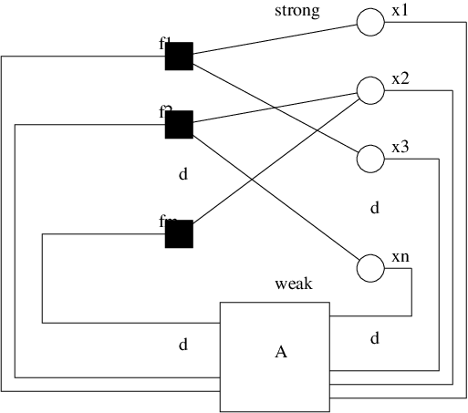
Together, and comprise the set of all indices for which a variable node is connected to the factor node in the graph . The union is thus the neighbor set of . Similarly, for any variable node , we let (with some abuse of notation) be the set of all indices for which a factor node is connected to via a strong edge, and let be the set of all indices for which there exists a weak edge. The union is thus the neighbor set of .
Given these definitions, we are interested in two problems:
- •
Optimization problem P-OPT: Given a function of the form (2) and a matrix , compute the maximum:
(4) Also, for each , compute the marginal value function
(5) where is composed of .
- •
Expectation problem P-EXP: Given a function of the form (2), a matrix , and scale factor , define the joint density
(6) where is a normalization constant called the partition function (which is a function of ). Then, for this density, compute the expectations
(7) Also, for each , compute the log marginal
(8) We include the scale factor so that the definition of allows an arbitrary scaling, as in (4).
We now show that P-OPT and P-EXP commonly arise in statistical inference. Suppose that we are given a probability density of the form (6) for some function . The function may depend implicitly on some observed vector , so that represents the posterior density of given . In this context, the solution to the problem P-OPT is precisely the maximum a posteriori (MAP) estimate of and given the observations . Similarly, the solution to the problem P-EXP is precisely the minimum mean squared error (MMSE) estimate. For P-EXP, the function is the log marginal density of .
The two problems are related: A standard large deviations argument [29] shows that, under suitable conditions, as the density in (6) concentrates around the maxima in the solution to the problem P-OPT. As a result, the solution to P-EXP converges to the solution to P-OPT.
II-A Further Assumptions and Notation
In the analysis below, we will assume that, for each factor node , we have that
| (9) |
i.e., the strong and weak neighbor sets are disjoint. This assumption introduces no loss of generality: If an edge is both weak and strong, we can modify the function to “move” the influence of from the term into the direct term . For example, suppose that, for some ,
In this case, the edge is both strong and weak. That is, the function depends on through both and through . To satisfy assumption (9), we define
under which . Thus we can replace and with and that obey (9).
Even when the dependence of a factor on a variable is only through the linear term , we may still wish to “move” the dependence to a strong edge. The reason is that the HyGAMP algorithm is designed around the assumption that the linear dependence is weak, i.e., that the elements in are small. If these elements are not small, then modeling the dependence with a strong edge improves the accuracy of HyGAMP at the expense of greater computation.
One final notation: since only when , we may sometimes write the summation (3) as
| (10) |
where is the sub-vector of with components and is the corresponding sub-matrix of .
III Motivating Examples
We begin with a basic development to show that problems with a fully separable prior and likelihood fit within our model. Then we show an extension to more complicated problems. More detailed examples are deferred to Sections VI and VII.
Linear Mixing and General Output Channel—Independent Sub-Vectors
As a simple example of a graphical model with linear mixing, consider the following estimation problem: An unknown vector has independent sub-vectors , each with a joint probability density . The vector is passed through a linear transform to yield an output . Each sub-vector then randomly generates an output with conditional density . The goal is to estimate given , the observations , and knowledge of the densities.
Common applications of this formulation include the following. In compressive sensing [22], is a sparse vector and is a sensing matrix. The measurements are usually modeled as plus Gaussian noise, in which case is Gaussian. In binary linear classification [30], the rows of are training feature vectors, the elements of are binary training labels, and is a weight vector learned to predict a label from its feature vector. Here, is an “activation function” that accounts for error in the linear-prediction model, often based on the logistic sigmoid. When , a sparse weight vector is sought to avoid over-fitting [31]. In digital communications settings, might be a vector of finite-alphabet symbols and a matrix representing the cumulative effect of the modulation, propagation channel, and demodulation [20]. Alternatively, might represent the channel impulse response, in which case is constructed from a training symbol sequence [13]. In either case, is usually chosen as Gaussian, although a heavy-tailed distribution can be chosen to model impulsive noise [17].
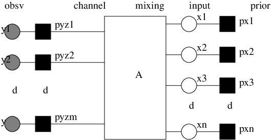
Under the assumption that the components are independent and the components are conditionally independent given , the posterior density on factors as
where is a normalization constant. For a fixed observation , we can write this posterior as
where is the log posterior, i.e.,
and the dependence on is implicit. The log posterior is therefore in the form of (2) with scale factor and factors . The first factors can be assigned as
| (11) |
which do not directly depend on the terms . Thus for each . The remaining factors are then
| (12) |
For these factors, the strong edge set is the singleton for , and there is no linear term; we can think of as zero-dimensional. The corresponding factor graph with the factors is shown in Fig. 2.
Linear Mixing and General Output Channel—Dependent Sub-Vectors
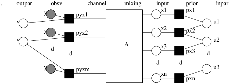
We now consider the significantly more general graphical model framework shown in Fig. 3. In this case, the input sub-vectors may be statistically dependent on one another, with dependences described by a graphical model. Some additional latent variables, in a vector , may also be involved. For example, [12] used a discrete Markov chain to model clustered sparsity, [16] used discrete-Markov and Gauss-Markov chains to model slow changes in support and amplitude across multiple measurement vectors, and [14] used a discrete Markov tree to model persistence across scale in the wavelet coefficients of an image. In Section VI, we will detail the application of HyGAMP to group sparsity.
Similarly, the likelihood need not be separable in . For example, the observations can depend on the outputs through a second graphical model that may include additional latent variables . For example, the distribution of given may depend on unknown parameters that also affect the distribution of given . This technique was used in [13] to incorporate constraints on LDPC coded bits when performing turbo sparse-channel estimation, equalization, and decoding using GAMP. In Section VII, we will detail the application of HyGAMP to multinomial logistic regression.
IV Review of Loopy Belief Propagation
Finding exact solutions to high-dimensional P-OPT and P-EXP problems is generally intractable because they require optimization or expectation over variables . A widely-used approximation method is loopy BP [32, 3], which reduces the high-dimensional problem to a sequence of low-dimensional problems associated with each factor . We consider two common variants of loopy BP: the max-sum algorithm (MSA) for the problem P-OPT and the sum-product algorithm (SPA) for the problem P-EXP. This section will briefly review these methods, as they will be the basis of the HyGAMP algorithms described in Section V.
The MSA iteratively passes estimates of the marginal utilities in (5) along the graph edges. Similarly, the SPA passes estimates of the log marginals in (8). For either algorithm, we index the iterations by and denote the “message” from the factor node to the variable node in the th iteration by and the reverse message by .
To describe the message updates, we introduce some additional notation. First, we note that SPA and MSA messages are equivalent up to a constant offset. That is, adding any constant (w.r.t. ) to either or has no effect on the algorithm. Thus, we will use “” for equality up to a constant offset, i.e.,
for some constant that does not depend on . Similarly, we write when for some constant . Finally, for the SPA, we will fix the scale factor in the problem P-EXP, and, for any function , we will write to denote the expectation of with respect to the density associated with :
| (14) | ||||
| (15) |
Given these definitions, the updates for the MSA and SPA variants of loopy BP are as follows:
Algorithm 1
Loopy BP: Consider the problems P-OPT or P-EXP above for some function of the form (2) and matrix . For the problem P-EXP, fix the scale factor . The MSA for P-OPT and the SPA for P-EXP iterate the following steps:
- 0)
Initialization: Set and, for each , set .
- 1)
Factor node update: For each edge , compute the function
(16) For the MSA, compute:
(17) where the maximization is over all variables with and subject to the constraint .
For the SPA, compute:
(18) where the integration is over all variables with , and is the probability density
(19) - 2)
Variable node update: For each :
(20) Also, let
(21) For the MSA, compute:
(22) For the SPA, compute:
(23) - 3)
Increment and return to Step 1 unless a maximum number of iterations is exceeded.
When the graph is acyclic, it can be shown that the MSA and SPA algorithms above converge to the exact solutions to the P-OPT and P-EXP problems, respectively. When the graph has cycles, however, the above algorithms are—in general—only approximate, but often quite accurate. The previous two statements assume that the loopy-BP messages are computed exactly, which is feasible when all variables are either Gaussian or discrete, but otherwise difficult—incurring a complexity that is exponential in general. For more details on loopy BP, see [32, 3, 33].
V Hybrid GAMP
The HyGAMP algorithm modifies loopy BP by replacing the weak edges with approximations of their cumulative effects. By treating a subset of dependencies as weak (as in AMP) rather than strong (as in loopy BP), the complexity of handling those dependencies shrinks from exponential in to linear in . In particular, HyGAMP assumes the elements of are small along any weak edge . Under this assumption, MSA-HyGAMP uses a quadratic approximation of the messages along the weak edges, reducing the factor-node update to a standard least-squares problem. Similarly, SPA-HyGAMP uses a Gaussian approximation of the weak-edge messages and applies the CLT at the factor nodes.
A derivation of the HyGAMP algorithm is given in Appendix A for the SPA and Appendix B for the MSA. We note that these derivations are “heuristic” in the sense that we do not claim any formal matching between loopy BP and the HyGAMP approximation.
To state the HyGAMP algorithm, we need additional notation. At iteration , the HyGAMP algorithm produces estimates and of the vectors and . Several other intermediate vectors, , and , are also produced. Associated with each of these vectors are matrices like and that represent Hessians for the MSA and covariances for the SPA. When referring to the inverses of these matrices, we use the notation to mean . Finally, for any positive definite matrix and vector , we define , which is a weighted two norm.
Algorithm 2
HyGAMP: Consider the problem P-OPT or P-EXP for some function of the form (2) and matrix . For the problem P-EXP, fix the scale factor . The MS-HyGAMP algorithm for P-OPT and the SP-HyGAMP algorithm for P-EXP iterate the following steps:
- 0)
Initialization: Set and , and select some initial values for each strong edge , and and for each index .
- 1)
Variable node update, strong edges: For each strong edge , compute
(24) - 2)
Variable node update, weak edges: For each variable node , compute
(25) and
(26) For MS-HyGAMP,
(27a) (27b) For SP-HyGAMP,
(28a) (28b) - 3)
Factor node update, linear step: For each factor node , compute
(29a) (29b) (29c) - 4)
Factor node update, strong edges: For each strong edge , compute:
(30) Then, for MS-HyGAMP, compute:
(31) where the maximization is jointly over and all components with .
For SP-HyGAMP, compute:
(32) where the integral is over and all components with , and is the probability density
(33) - 5)
Factor node update, weak edges: For each factor node , compute
(34a) Then, for MS-HyGAMP, compute: (34b) (34c) where the maximization in (34b) is over the sub-vector and output vector .
For SP-HyGAMP, let
(35) where is the component of the pair with the joint density
(36) Then, for either MS-HyGAMP or SP-HyGAMP compute
(37a) (37b) - 6)
Variable node update, linear step: For each variable node compute
(38a) (38b) Increment and return to Step 1 unless either a maximum number of iterations is exceeded or is sufficiently small.
Although the HyGAMP algorithm above appears much more complicated than standard loopy BP (Algorithm 1), HyGAMP can require dramatically less computation. Recall that the main computational difficulty of loopy BP is Step 1, the factor update. The updates (17) and (18) involve an optimization or expectation over sub-vectors, where is the set of all sub-vectors connected to the factor node . In the HyGAMP algorithm, these computations are replaced by (31) and (32), where the optimization and expectation need only be computed over the strong edge sub-vectors . If the number of weak edges is large, the computational savings can be dramatic. The other steps of the HyGAMP algorithms are all linear, simple least-square operations, or componentwise nonlinear functions on the individual sub-vectors.
For ease of illustration, we have only presented one form of the HyGAMP procedure. Several variants are possible:
- •
Discrete distributions: The above description assumed continuous-valued random variables . The procedures can be easily modified for discrete-valued variables by appropriately replacing integrals with summations.
- •
Message scheduling: The above description also only considered a completely parallel implementation where each iteration performs exactly one update on all edges. Other so-called message schedules are also possible and may offer more efficient implementations or better convergence depending on the application (e.g., [34, 35, 36]).
VI Application to Group-Sparse Signal Recovery
To illustrate the HyGAMP method, we first consider the group-sparse estimation problem [37, 38]. Although this problem does not utilize the full generality of HyGAMP, it provides a simple example of the HyGAMP method and has a number of existing algorithms that can be compared against.
VI-A HyGAMP Algorithm
A general version of the group-sparsity problem that falls within the HyGAMP framework can be described as follows. Let be an -dimensional vector with scalar components . Vector-valued components could also be considered, but we restrict our attention to scalar components for simplicity. The component indices of the vector are divided into (possibly overlapping) groups, . We let be the set of group indices such that . That is, is the set of groups to which the component belongs.
Suppose that each group can be “active” or “inactive”, and each component can be non-zero only when at least one group is active for some . Qualitatively, a vector is sparse with respect to this group structure if it is consistent with only a small number of groups being active. That is, most of the components of are zero with the non-zero components having support contained in a union of a small number of groups. The group-sparse estimation problem is to estimate the vector from some measurements . The traditional (non-group) sparse estimation problem corresponds to the special case when there are groups of singletons, .
There are many ways to model the group-sparse structure in a Bayesian manner, particularly with overlapping groups. For sake of illustration, we consider the following simple model. For each group , let be a Boolean variable with when the group is active and when it is inactive. We call the “activity indicators” and model them as i.i.d. with
| (39) |
for some sparsity rate . We assume that, given the vector , the components of are independent with the conditional densities
| (40) |
where is a random variable having the distribution of the component in the event that it belongs to an active group. Finally, suppose that measurement vector is generated by first passing through a linear transform and then a separable componentwise measurement channel with likelihoods . Many other dependencies on the activities of and measurement models are possible – we use this simple model for illustration.
Under this model, the prior and the measurements are naturally described by a graphical model with linear mixing. Due to the independence assumptions, the posterior density of given factors as
| (41) |
where is the conditional density for the random variable in (40). The factor graph corresponding to this distribution is shown in Fig. 4.

Under this graphical model, Appendix C shows that SP-HyGAMP from Algorithm 2 reduces to the simple procedure outlined in Algorithm 3. A similar MS-HyGAMP variant could also be derived. In lines 8 and 9 of Algorithm 3, we used and to denote the expectation and variance, respectively, of the scalar random variable with density
| (42) |
and is an AWGN corrupted version of ,
| (43) |
Algorithm 3 can be interpreted as the GAMP procedure from [8] with an additional update of the sparsity rates. Specifically, each iteration of the algorithm has two stages. The first stage, labeled as the “basic GAMP update,” contains the updates from the basic GAMP algorithm [8], which treats the components as independent with sparsity rate . The second stage of Algorithm 3, labeled as the “sparsity-rate update,” updates the sparsity rates based on the estimates returned by the first stage.
The second stage of Algorithm 3 has a simple interpretation. The quantities and can be interpreted, respectively, as estimates for the probabilities
That is, is an estimate of the probability that the component belongs to at least one active group and is an estimate of the probability that it belongs to an active group other than . Similarly, the quantities and are estimates for the log likelihood ratios
Most of the updates in the second stage are natural conversions from LLR values to estimates of and . In line 21, the LLR message is computed as
| (44) |
where is the probability density for the scalar random variable in (43), where has the density (42). The message (44) is the ratio of two likelihoods: the likelihood that belongs to an active group and the likelihood that belongs to an active group other than .
To summarize, Algorithm 3 provides a simple and intuitive way to extend the basic GAMP algorithm of [8] to group-structured sparsity.
The HyGAMP algorithm for group sparsity is also extremely general. The algorithm can apply to arbitrary priors and output channels. In particular, the algorithm can incorporate logistic outputs that are often used for group sparse classification problems [39, 40, 41]; details are provided in [42]. Also, the method can handle arbitrary, even overlapping, groups. In contrast, the extensions of other iterative algorithms to the case of overlapping groups sometimes requires approximations; see, for example, [43]. In fact, the methodology is quite general and likely may be applied to general structured sparsity, including possibly the graphical-model-based sparse structures in image processing considered in [44].
VI-B Computational Complexity
In addition to its generality, the HyGAMP procedure is among the most computationally efficient for group sparsity. To illustrate this point, consider the special case when there are non-overlapping groups of elements each. In this case, the total vector dimension for is . We consider the non-overlapping case since there are many algorithms that apply to this case that we can compare against. For non-overlapping uniform groups, Table I compares the computational cost of the HyGAMP algorithm to other methods.
The computational cost of each iteration of the HyGAMP algorithm, Algorithm 3, is dominated by the matrix multiplications by (line 10) and (line 18) and by the componentwise squares of and (lines 11 and 17). Each of these operations has cost. Note that the multiplications by componentwise-square matrices can be eliminated by using the scalar-variance version of GAMP [8]. Also, the multiplications by and are relatively cheap if the matrix has a fast transform (e.g., FFT). The other per-iteration computations are the scalar estimates at the output (lines 13 and 14); the scalar estimates at the input (lines 8 and 9); and the updates of the LLRs. All of these computations are relatively simple.
For the case of non-overlapping groups, the HyGAMP algorithm could also be implemented using vector-valued components. Specifically, the vector can be regarded as a block vector with vector components, each of dimension . The general HyGAMP algorithm, Algorithm 2, can be applied on the vector-valued components. To contrast this with Algorithm 3, we will call Algorithm 3 HyGAMP with scalar components, and call the vector-valued case HyGAMP with vector components.
The cost is slightly higher for HyGAMP with vector components. In this case, there are no non-trivial strong edges since the block components are independent. However, in the update (29c), each is and is . Thus, the computation (29c) requires computations of cost each for a total cost of , which is the dominant cost. Of course, there may be a benefit in performance for HyGAMP with vector components, since it maintains the complete correlation matrix of all the components in each group. We do not investigate this possible performance benefit in this paper.
Also shown in Table I is the cost of the relaxed BP method from [45], which also uses approximate message passing similar to HyGAMP with vector components. That method, however, performs the same computations as HyGAMP on each of the graph edges as opposed to the graph vertices. It can be verified that the resulting cost has an term.
| Method | Complexity |
|---|---|
| Group-OMP [46] | |
| Group-Lasso [37, 38, 47] | per iteration |
| Relaxed BP with vector components [45] | per iteration |
| HyGAMP with vector components | per iteration |
| HyGAMP with scalar components | per iteration |
These message passing algorithms can be compared against widely-used group LASSO methods [37, 38], which estimate by solving some variant of a regularized least-squares problem of the form
| (45) |
for some regularization parameter . The problem (45) is convex and can be solved via a number of methods including [48, 49, 47], the fastest of which is the SpaRSA algorithm of [47]. Interestingly, this algorithm is similar to the GAMP method in that the algorithm is an iterative procedure, where in each iteration there is a linear update followed by a componentwise scalar minimization. Like the GAMP method, the bulk of the cost is the operations per iteration for the linear transform. An alternative approach for group sparse estimation is group orthogonal matching pursuit (Group-OMP) of [46, 41], a greedy algorithm that detects one group at a time. Each round of detection requires correlations of cost . If there are on average nonzero groups, the total complexity will be . From the complexity estimates summarized in Table I it can be seen that GAMP, despite its generality, is computationally as simple (per iteration) as some of the most efficient algorithms specifically designed for the group sparsity problem.
Of course, a complete comparison requires that we consider the number of iterations, not just the computation per iteration. This comparison requires further study beyond the scope of this paper. However, it is possible that the HyGAMP procedure will be favorable in this regard. Our simulations below show good convergence after only 10–20 iterations. Moreover, in the case of independent (i.e. non-group) sparsity, the number of iterations for AMP algorithms is typically small and often much less than other iterative methods. Examples in [22] show excellent convergence in to iterations, which is dramatically faster than the iterative soft-thresholding method of [50].
VI-C Numerical Experiments
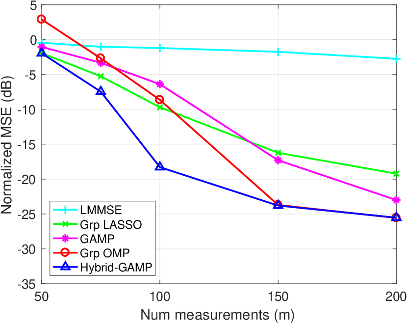
Fig. 5 shows a simple simulation comparison of the mean squared error (MSE) of the HyGAMP method (Algorithm 3) along with group OMP, group LASSO, basic GAMP, and the simple linear MMSE estimator. The simulation used a vector with groups of size and sparsity fraction of . The matrix was i.i.d. Gaussian and the observations were with AWGN noise at an SNR of 20 dB. The number of measurements was varied from 50 to 200, and the plot shows the MSE for each of the methods. The HyGAMP method was run with 20 iterations. In group LASSO, at each value of , the algorithm was simulated with several values of the regularization parameter in (45) and the plot shows the minimum MSE. In Group-OMP, the algorithm was run with the true value of the number of nonzero coefficients. It can be seen that the HyGAMP method is consistently as good or better than both other methods. Furthermore, HyGAMP is significantly better than basic GAMP, which exploits sparsity but not group sparsity. All code for the simulations can be found in the GAMPmatlab package [51].
We conclude that, for the problem of group-sparse recovery from AWGN-corrupted measurements, the HyGAMP method is at least comparable in performance and computational complexity to the most competitive algorithms. On top of this, HyGAMP offers a much more general framework that can include more rich modeling in both the output and input.
VII Application to Multinomial Logistic Regression
In a second example of the HyGAMP method, we apply it to the problem of multiclass linear classification using the approach known as multinomial logistic regression.
VII-A Multinomial Logistic Regression
In multiclass classification [30], one observes a training set consisting of pairs of a feature vector and a -ary class label . The goal is then to infer the unknown -ary class label of an observed feature vector . In the linear approach to this problem, we design a weight matrix from the training set. Then, given an unlabeled feature vector , we first generate a vector of linear “scores” , and estimate the class label as the index of the largest score, i.e.,
| (46) |
Multinomial linear regression (MLR) [30] is one of the best known methods to design the weight matrix . There, the labels are modeled as conditionally independent given the scores , where . That is,
| (47a) | |||
| where is the multinomial logistic pmf, | |||
| (47b) | |||
The rows of the weight matrix are then modeled as i.i.d.,
| (48) |
For log-convex , MAP estimation of is a convex problem. The log-convex Laplacian prior
| (49) |
is a popular choice for that promotes sparsity in the designed weight matrix . Sparsity is essential in the case that the feature dimension is much larger than the number of training examples . Fast implementations of sparse MLR were proposed in [31] and refined in [52].
VII-B HyGAMP Algorithm
Max-sum HyGAMP (MS-HyGAMP) can be directly applied to solve the above optimization problem. To do this, we set and, recalling (11), we choose , and recalling (12), we choose . Then (27a) boils down to
| (50) |
and (34b) boils down to
| (51) |
Both problems are convex and can be solved using standard methods, e.g., majorization–minimization or Newton’s method in the case of (51). For more details, including the implementation of (27b) and (34c), we refer the reader to [53].
SP-HyGAMP can also be applied to MLR, again using the likelihood (47). However, rather than the Laplacian prior (49), we suggest choosing the Bernoulli-multivariate-Gaussian prior
| (52a) | ||||
| (52b) | ||||
with , which promotes approximate row-sparsity in under sum-product inference. In this case, it can be shown [53] that (28) can be computed in closed form as
| (53) | ||||
| (54) | ||||
| (55) |
Although we are not aware of a closed-form solution to (35), it can be approximated using numerical integration.
VII-C Numerical Experiments
We will now describe the results of two experiments used to evaluate the application of HyGAMP to sparse MLR. In these experiments, SP-HyGAMP and MS-HyGAMP were compared to two state-of-the-art sparse MLR algorithms: SBMLR from [54] and GLMNET from [52].
VII-C1 Synthetic Data
We first performed an experiment on synthetic data with classes, features, and examples. The use of synthetic data allowed us to analytically compute the expected test-error rate associated with the designed weight matrices .
To generate the synthetic data, we first constructed the set of training labels such that training samples were dedicated to each class. Then we drew feature vectors i.i.d. from the class-conditional density . The class means were -sparse, with support chosen uniformly at random and with non-zero entries chosen uniformly from the columns of a random orthonormal matrix. The parameter was then chosen to achieve a Bayes error rate of . Thus, only of the features were discriminatory. Note that the data-generation model is not matched to the statistical model assumed in the derivation of MS-HyGAMP or SP-HyGAMP.
To test the algorithms, we performed trials, where in each trial we invoked each algorithm-under-test on randomly generated training data and then computed the resulting expected test-error rate. The SP-HyGAMP algorithm used (52) with parameters tuned over a logarithmically-spaced grid using 5-fold cross-validation (CV). The GLMNET algorithm, which solves the same convex optimization problem as MS-HyGAMP, tuned in (49) over logarithmically-spaced values using -fold CV. The same CV-optimal was then used for MS-HyGAMP. Finally, SBMLR is parameter-free, and thus did not require tuning.
For a designed weight matrix , the expected test-error rate can be analytically computed [53] as
| (56) | ||||
| (57) |
where and the multivariate normal cdf in (57) was computed using Matlab’s mvncdf.
In addition to computing the expected test-error rate, we computed two metrics for the sparsity of the designed weight matrices. The metric quantifies absolute sparsity, i.e., the number of non-zero elements in . But since the weights returned by SP-HyGAMP are non-zero with probability one, we also computed the “effective sparsity” , which is defined as the minimum number of elements in required to reach of .
Table II shows the expected test-error rate, , and of each algorithm, averaged over 12 independent trials. From this table, we see that MS-HyGAMP and GLMNET matched on all metrics. This result is expected because the two algorithms aim to solve the same convex problem, and it offers evidence that they do in fact solve the problem. Thus, in the sequel, we report only the results of GLMNET. Next, Table II shows that the SP-HyGAMP achieved the best expected test-error rate of , with SBMLR achieving the second best. For comparison, we recall that the Bayes (i.e., minimum) expected error rate was in this experiment. The table also shows that the (average) effective sparsity was similar for all algorithms, and smaller than the sparsity of the Bayes’ optimal classifier for this dataset, which is .
| Algorithm | % Error | ||
|---|---|---|---|
| GLMNET | 14.787 | 13.25 | 25.75 |
| MS-HyGAMP | 14.787 | 13.25 | 25.75 |
| SBMLR | 14.059 | 15.08 | 28.92 |
| SP-HyGAMP | 13.981 | 16.08 | 1500 |
VII-C2 Handwritten Digit Classification
In the second experiment, we tested SP-HyGAMP, GLMNET, and SBMLR on the Mixed National Institute of Standards and Technology (MNIST) dataset[55]. The MNIST dataset consists of total images of handwritten digits through , hence . Each image has pixels. In this experiment we performed 24 trials, where in each trial we randomly partitioned the total dataset into a training and testing portion. Within each trial, we varied the number of image samples in the training partition from to . Using the training data, we used each algorithm-under-test to design a weight matrix, which was then used to compute an empirical error-rate on the test partition of the dataset. In this experiment, SP-HyGAMP and GLMNET tuned their associated parameters in a similar manner as in the synthetic experiment. However, they used -fold CV instead of -fold CV to reduce computation.
Figure 6 shows the empirical test-error rate versus the number of training samples , averaged over the random trials. The error bars indicate the standard deviation of the empirical error-rate estimate. The figure shows that, for all , SP-HyGAMP achieved the best test-error rate and GLMNET achieved the second best. The figure also shows that, for all algorithms, the test-error rate decreased to a common value as the number of training samples increased. This is not surprising; we expect that, with enough training data, any reasonable approach should recover a close approximation to the Bayes-optimal linear classifier. A much more difficult problem is designing a good linear classifier from limited training data, and, for this problem, Figure 6 shows that SP-HyGAMP beats the competition.

VII-D Simplified HyGAMP and EM/SURE Tuning
When directly applied to multinomial logistic regression, each iteration of HyGAMP involves the update of multivariate Gaussian pdfs, each of dimension , for a total complexity of per iteration. This complexity can be quite large in practice, especially relative to state-of-the-art methods like GLMNET and SBMLR. Furthermore, in its more direct form, HyGAMP assumes knowledge of the statistical parameters of its prior and likelihood. In order to tune these parameters to the data, it was suggested above to use cross-validation (as with GLMNET). But -fold cross-validation of parameters using hypothesized values of each parameter requires the training and evaluation of classifiers, which can be very expensive in practice.
Fortunately, for multinomial logistic regression, it is possible to modify HyGAMP in such a way that the complexity of the resulting method becomes competitive with GLMNET and SBMLR. The modification consists of two parts: i) a simplification of HyGAMP wherein the covariance matrices are constrained to be diagonal; and ii) an application of EM-based [56] and SURE-based [57] parameter tuning to the priors and likelihoods relevant to multinomial logistic regression. A complete description of EM/SURE-tuned simplified HyGAMP (SHyGAMP) for multinomial logistic regression can be found in [58], with full derivations in [53]. In [58], a detailed numerical study establishes that EM/SURE-tuned SHyGAMP is competitive in both performance and complexity with GLMNET and SBMLR. Due to space limitations, we refer the interested reader to [53] and [58] for more details.
We conclude by saying that, although the “direct” application of HyGAMP from Section V may not lead to a complexity that is always competitive with state-of-the-art methods, it acts as an important first step in deriving simplified and/or enhanced version of HyGAMP. This underscores the importance of HyGAMP as stated in Section V.
VIII Conclusions
A general model for optimization and statistical inference based on graphical models with linear mixing was presented. The linear mixing components of the graphical model account for interactions through aggregates of large numbers of small, linearizable perturbations. Gaussian and second-order approximations are shown to greatly simplify the implementation of loopy BP for these interactions, and the HyGAMP framework presented here enables these approximations to be incorporated in a systematic manner in general graphical models. Simulations were presented for group sparsity and multinomial logistic regression, where the HyGAMP method has equal or superior performance to existing methods. Although we saw that, in multinomial logistic regression, a direct application of HyGAMP does not lead to state-of-the-art computationally complexity, a modification of the HyGAMP presented here suffices to address the complexity issue [53, 58]. The generality of the proposed HyGAMP algorithm also allows its application to many other problems beyond these two examples, such as multiuser detection in massive MIMO [23, 24], inference for neuronal connectivity [25], fitting neural mass spatio-temporal models [26], user activity detection in cloud-radio random access [27], and decoding from pooled data [28]. In addition to pursuing such applications, future work will focus on establishing rigorous theoretical analyses along the lines of [7, 8] for specific instances of HyGAMP.
Appendix A Derivation of SP-HyGAMP
A-A Preliminary Lemma
Before deriving the SP-HyGAMP algorithm, we need the following result. Let be a real-valued function of vectors and of the form
| (58) |
for some positive definite matrix .
Lemma 1
Suppose that and are random vectors with a conditional probability distribution function of the form
where is given in (58), is some constant and is a normalization constant (called the partition function). Then,
| (59a) | |||||
| (59b) | |||||
| (59c) | |||||
| where | |||||
Proof:
The relations are standard properties of exponential families [3].
A-B SP-HyGAMP Approximation
First partition the objective function in (16) as
| (60) | |||||
where
| (61a) | |||||
| (61b) | |||||
That is, we have separated the terms in between the strong and weak edges.
Then, the marginal distribution of the distribution in (19) can be re-written as
| (62) | |||||
where
| (63a) | |||||
| (63b) | |||||
and the integration in (63a) is over the variables with , and and the integration in (63b) is over the variables with , and .
To approximate in (62), we separately consider the cases when is weak edge and when it is a strong edge. We begin with the weak edge case. That is, . Let
| (64a) | |||||
| (64b) | |||||
| (64c) | |||||
| (64d) | |||||
where we have used the notation from (14).
Now, using the expression for in (61b), it can be verified that is equivalent to the probability distribution of a random variable
| (65) |
with the variables being independent with probability distribution
Moreover, and in (64) are precisely the mean and variance of the random variables under this distribution. Therefore, if the summation in (65) is over a large number of terms, we can then use the CLT to approximate the variable in in (65) as Gaussian, with distribution given by
| (66) |
where
| (67a) | |||||
| (67b) | |||||
Substituting this Gaussian approximation into the probability distribution in (19), and then using the definitions in (61a) and (63a), we obtain the following approximation of the message in (18),
| (68) |
where
| (69) | |||||
and where is given in (34a).
Now define
| (70a) | |||||
| (70b) | |||||
so that the expressions in (67) can be re-written as
| (71a) | |||||
| (71b) | |||||
Also, let
| (72a) | |||||
| (72b) | |||||
Using Lemma 1, one can show that the definitions in (72) agree with the updates (37) where and are the mean and covariance of the random variable with the distribution (36).
Next consider the case when so that is a strong edge. In this case, does not depend on and a similar calculation as above shows that
| (74) |
where and are defined in (70). Substituting the Gaussian approximation (74) into (19), and then using the definitions in (61a) and (63a), one can show that the marginal distribution in (19) is equal to the marginal distribution of in (33). Therefore, the message in (18) can be written as (32) for all strong edges .
We now turn to the variable node update (20) which we partition as
| (75) |
where
| (76a) | |||||
| (76b) | |||||
Substituting the approximation (73) into (76b) gives
| (77) |
where
| (78a) | |||||
| (78b) | |||||
We again consider the case of a weak edge separately from a strong edge. When is weak edge, , so that in (76a) does not depend on . Combining (75) and (77), we see that
| (79) |
where is defined in (26). Also, comparing (38) with (78), we have that
| (80a) | |||||
| (80b) | |||||
Substituting (80) into (79) we get
| (81) | |||||
A similar set of calculations shows that in (21) can be approximated as
| (82) |
Appendix B Derivation of MS-HyGAMP
The derivation of MS-HyGAMP is similar to the derivation of SP-HyGAMP in Appendix A.
B-A Preliminary Lemma
Lemma 2
Assume the maximization in (87) exists and is unique and twice differentiable. Then,
| (88a) | |||||
| (88b) | |||||
| (88c) | |||||
where
Proof:
Since is a maximizer of ,
| (89) |
Therefore, (88a) follows from
where the last step is a result of the form of in (58). The form of in (58) also shows that for all and
Taking the derivative of (89),
which implies that
which proves (88b). Finally, taking the second derivative of (88a) along with (88b) shows (88c).
B-B MS-HyGAMP Approximation
Similar to the SPA derivation, we first partition the function in (16) as in (60). We can also partition the maximization (17) as
| (90) | |||||
where
| (91a) | |||||
| (91b) | |||||
with the maximization in (91a) being over all with ; and the maximization in (91b) over all with subject to . The partitioning (90) is valid since the strong and weak edges are distinct. This insures that for all , either or , but not both.
The HyGAMP approximation applies to the weak term (91b). For any and all weak edges , define:
| (92a) | |||||
| (92b) | |||||
| (92c) | |||||
| (92d) | |||||
which are the maximum and Hessian of the incoming weak messages. Since the assumption of the HyGAMP algorithm is that is small for all weak edges , the values of in the maximization (91b) will be close to . So, for all weak edges, , we can approximate each term in (61b) with the second-order approximation
| (93) | |||||
where we have additionally made the approximation for all . Substituting (93) into (61b), the maximization (91b) reduces to
| (94) | |||||
where the constant term does not depend on or .
To proceed, we need to consider two cases separately: when and when . First consider the case when . That is, is a weak edge. In this case, a standard least-squares calculation shows that (94) reduces to
| (95) | |||||
where and are given in (67). Also, when , the assumption that and are disjoint implies that . In this case, in (91a) with the objective function (61a) will not depend on , so we can write
| (96) | |||||
where the maximization is over all for . Combining (90), (95) and (96), we can write that, for all weak edges ,
| (97) |
where
| (98) |
and is defined in (34a).
Now define and as in (70). Using (71), neglecting terms of order , and taking the approximation that , (97) can be further approximated as
similar to (68). Now, similar to (72), let
| (99a) | |||||
| (99b) | |||||
Based on the definition of in (98) with defined in (34a), one can apply Lemma 2 to show that (99) agrees with (37). Using a similar approximation as in the derivation of the SPA-HyGAMP, one can then obtain the quadratic approximation in (73) for for all weak edges .
Next consider the case when so that is a strong edge. In this case, in (94) does not depend on , so we can write
| (100) |
where
| (101) |
with the maximization being over such that . Using a similar least-squares calculation as above, is given by
| (102) |
and and are defined in (70). Combining (90), (100) and (102), we can write that, for all strong edges ,
| (103) | |||||
From (61a) and (91a), we see that (103) agrees with the factor node update (31) for the strong edges.
Appendix C Derivation of HyGAMP for Group Sparsity
This appendix provides a brief explanation of how the steps in Algorithm 3 were obtained from SP-HyGAMP in Algorithm 2. In the description of the SP-HyGAMP algorithm, we used labels and for the factor and variable nodes. However, the group-sparse estimation problem introduces many other indices. To avoid confusion, we adopt the following more explicit (albeit somewhat more cumbersome) labeling. The variables nodes will be labeled explicitly by or . For the factor nodes, we use the labels:
- •
for the factors ;
- •
for the factors ; and
- •
for the factors .
With this convention, for example, represents the message from the variable node to the factor node when .
Now, in the graphical model in Fig. 4, the strong edges are all the edges to the right of the variables . That is, the strong edges are:
- •
between the variables and factors for all ;
- •
between the variables and factors for all ; and
- •
between the variables and factors for all .
The remaining edges, those between the variables and the factor nodes , are all weak.
With these definitions, we can easily derive the steps in Algorithm 3 from SP-HyGAMP in Algorithm 2. First, note that all the steps from lines 10–18 are simply the weak edge updates from Algorithm 2 specialized to the case of scalar variables.
To understand the role of the remaining lines, first consider the message along the strong edge from the factor node and the variable . The factor node corresponds to the prior in (39). Since the factor is attached to only one variable node, the outgoing message in (32) for this edge reduces to
where the last step follows from (39).
Next consider the message along the strong edge from the variable to the factor node for some . Similar to the case of binary LDPC codes [59], since or 1, it is convenient to work with log-likelihood ratios (LLRs). Given any strong edge between and , define the LLR,
| (109) |
The reverse LLR, is defined similarly.
Since the variable node is not connected to any weak edges, the variable node output message in (24) reduces to
Therefore the LLR in (109) is given by
| (110) | |||||
where the last step follows from (C).
Next consider the message from to . Recall that the factor node corresponds to the distribution , defined by the variable in (40). Also, this factor node has no weak edges. Hence, it can be verified that the message (32), propagating from factor node to variable , is given by
| (111) |
where is the probability density
| (112) |
and the expectation is over independent variables with
| (113) |
Using the fact that the is the conditional distribution for the variable in (40), the probability distribution in (112) can be written
| (114) |
where is the distribution for the variable in (42) and is the probability
| (115) | |||||
Now, the variable node has only one strong edge: that connecting it to the factor node . Therefore, the log probability in (25) reduces to
| (116) |
Now, as described in equations (111) and (114), is the log of the probability distribution for the variable in (42) with . Hence in (116) must be the log posterior distribution for the with the measurement in (43). Therefore, the expectations and variances in (28) agree with the expressions in lines 8 and 9.
Finally, consider the message from the factor node to a variable node . The derivation for this message is similar to the message from to . Specifically, it can be verified that the factor node message (32), applied to the strong edge from to , is given by
| (117) |
where is the probability mass function
| (118) | |||||
where the expectation is over independent variables with probabilities in (113). To evaluate the expectation on the right-hand side of (118), consider the conditional expectation . Since the distribution corresponds to the random variable in (40),
where is the probability distribution for the random variable in (42) and
| (122) | |||||
Also, the edge from variable node to the factor node is the only strong edge connected to . Therefore, the variable node message (24) applied to that edge reduces to
| (123) |
Substituting (C) and (123) into (118) we obtain that
where is the probability distribution of the scalar random variable in (43) with being distributed in (42). The LLR corresponding to (C) is thus given by
which agrees with (44).
References
- [1] S. Rangan, A. K. Fletcher, V. K. Goyal, and P. Schniter, “Hybrid generalized approximation message passing with applications to structured sparsity,” in Proc. IEEE Int. Symp. Inform. Theory, Cambridge, MA, Jul. 2012, pp. 1241–1245.
- [2] B. J. Frey, Graphical Models for Machine Learning and Digital Communication. MIT Press, 1998.
- [3] M. J. Wainwright and M. I. Jordan, “Graphical models, exponential families, and variational inference,” Found. Trends Mach. Learn., vol. 1, no. 1–2, pp. 1–305, 2008.
- [4] D. Koller and N. Friedman, Probabilistic Graphical Models: Principles and Techniques. Cambridge, MA: MIT Press, 2009.
- [5] D. L. Donoho, A. Maleki, and A. Montanari, “Message-passing algorithms for compressed sensing,” Proc. Nat. Acad. Sci., vol. 106, no. 45, pp. 18 914–18 919, Nov. 2009.
- [6] ——, “Message passing algorithms for compressed sensing I: Motivation and construction,” in Proc. Info. Theory Workshop, Jan. 2010, pp. 1–5.
- [7] M. Bayati and A. Montanari, “The dynamics of message passing on dense graphs, with applications to compressed sensing,” IEEE Trans. Inform. Theory, vol. 57, no. 2, pp. 764–785, Feb. 2011.
- [8] S. Rangan, “Generalized approximate message passing for estimation with random linear mixing,” in Proc. IEEE Int. Symp. Inform. Theory, Saint Petersburg, Russia, Jul.–Aug. 2011, pp. 2174–2178.
- [9] J. Parker, P. Schniter, and V. Cevher, “Bilinear generalized approximate message passing—Part I: Derivation,” IEEE Trans. Signal Processing, vol. 62, no. 22, pp. 5839–5853, 2013.
- [10] ——, “Bilinear generalized approximate message passing—Part II: Applications,” IEEE Trans. Signal Processing, vol. 62, no. 22, pp. 5854–5867, 2013.
- [11] J. Parker and P. Schniter, “Parametric bilinear generalized approximate message passing,” IEEE J. Sel. Topics Signal Proc., vol. 10, no. 4, pp. 1–14, 2016.
- [12] P. Schniter, “Turbo reconstruction of structured sparse signals,” in Proc. Conf. on Inform. Sci. & Sys., Princeton, NJ, Mar. 2010.
- [13] ——, “A message-passing receiver for BICM-OFDM over unknown clustered-sparse channels,” IEEE J. Sel. Topics Signal Process., vol. 5, no. 8, pp. 1462–1474, Dec. 2011.
- [14] S. Som and P. Schniter, “Compressive imaging using approximate message passing and a Markov-tree prior,” IEEE Trans. Signal Process., vol. 60, no. 7, pp. 3439–3448, Jul. 2012.
- [15] J. Ziniel and P. Schniter, “Efficient high-dimensional inference in the multiple measurement vector problem,” IEEE Trans. Signal Process., vol. 61, no. 2, pp. 340–354, Jan. 2013.
- [16] ——, “Dynamic compressive sensing of time-varying signals via approximate message passing,” IEEE Trans. Signal Process., vol. 61, no. 21, pp. 5270–5284, Nov. 2013.
- [17] M. Nassar, P. Schniter, and B. Evans, “A factor-graph approach to joint OFDM channel estimation and decoding in impulsive noise environments,” IEEE Trans. Signal Process., vol. 62, no. 6, pp. 1576–1589, Mar. 2014.
- [18] J. Vila, P. Schniter, and J. Meola, “Hyperspectral image unmixing via turbo bilinear approximate message passing,” IEEE Trans. Computat. Imaging, vol. 1, no. 3, pp. 143–158, 2015.
- [19] E. W. Tramel, A. Drémeau, and F. Krzakala, “Approximated message passing with restricted Boltzmann machine priors,” J. Stat. Mech.: Thy. Exp., vol. 2016, no. 7, p. 073401, 2016.
- [20] G. Caire, A. Tulino, and E. Biglieri, “Iterative multiuser joint detection and parameter estimation: a factor-graph approach,” in Proc. IEEE Inform. Theory Workshop, Cairns, Australia, Sep. 2001, pp. 36–38.
- [21] S. Rangan and R. Madan, “Belief propagation methods for intercell interference coordination,” in Proc. IEEE Infocom, Shanghai, China, Apr. 2011.
- [22] A. Montanari, “Graphical model concepts in compressed sensing,” in Compressed Sensing: Theory and Applications, Y. C. Eldar and G. Kutyniok, Eds. Cambridge Univ. Press, Jun. 2012, pp. 394–438.
- [23] S. Wang, Y. Li, and J. Wang, “Multiuser detection in massive spatial modulation MIMO with low-resolution ADCs,” IEEE Trans. Wireless Comm., vol. 14, no. 4, pp. 2156–2168, 2015.
- [24] S. Wang and L. Zhang, “Signal processing in massive MIMO with IQ imbalances and low-resolution ADCs,” IEEE Trans. Wireless Comm., vol. 15, no. 12, pp. 8298–8312, 2016.
- [25] A. K. Fletcher and S. Rangan, “Scalable inference for neuronal connectivity from calcium imaging,” in Proc. Neural Information Processing Systems, 2014, pp. 2843–2851.
- [26] A. K. Fletcher, J. Viventi, and S. Rangan, “Neural mass spatio-temporal modeling from high-density electrode array recordings,” in Proc. Information Theory and Applications Workshop, 2015, pp. 319–321.
- [27] Z. Utkovski, O. Simeone, T. Dimitrova, and P. Popovski, “Random access in c-ran for user activity detection with limited-capacity fronthaul,” IEEE Signal Process. Lett., vol. 24, no. 1, pp. 17–21, 2017.
- [28] A. E. Alaoui, A. Ramdas, L. Zdeborova, M. I. Jordan et al., “Decoding from pooled data: Phase transitions of message passing,” arXiv preprint arXiv:1702.02279, 2017.
- [29] A. Dembo and O. Zeitouni, Large Deviations Techniques and Applications. New York: Springer, 1998.
- [30] C. M. Bishop, Pattern Recognition and Machine Learning, ser. Information Science and Statistics. New York, NY: Springer, 2006.
- [31] B. Krishnapuram, L. Carin, M. Figueiredo, and A. Hartemink, “Sparse multinomial logistic regression: Fast algorithms and generalization bounds,” IEEE Trans. Pattern Anal. and Mach. Int., vol. 27, no. 6, pp. 957–968, 2005.
- [32] J. Pearl, Probabilistic Reasoning in Intelligent Systems: Networks of Plausible Inference. San Mateo, CA: Morgan Kaufmann Publ., 1988.
- [33] J. S. Yedidia, W. T. Freeman, and Y. Weiss, “Understanding belief propagation and its generalizations,” in Exploring Artificial Intelligence in the New Millennium. San Francisco, CA: Morgan Kaufmann Publishers, 2003, pp. 239–269.
- [34] D. M. Malioutov, J. K. Johnson, and A. S. Willsky, “Walk-sums and belief propagation in Gaussian graphical models,” J. Machine Learning Res., vol. 7, pp. 2031–2064, Oct. 2006.
- [35] G. Elidan, I. McGraw, and D. Koller, “Residual belief propagation: Informed scheduling for asynchronous message passing,” in Proc. Conf. on Uncertainty in AI, Boston, MA, Jul. 2006.
- [36] A. Manoel, F. Krzakala, E. W. Tramel, and L. Zdeborová, “Swept approximate message passing for sparse estimation,” in Proc. ICML, 2015, pp. 1123–1132.
- [37] M. Yuan and Y. Lin, “Model selection and estimation in regression with grouped variables,” J. Royal Statist. Soc., vol. 68, pp. 49–67, 2006.
- [38] P. Zhao, G. Rocha, and B. Yu, “The composite absolute penalties family for grouped and hierarchical variable selection,” Ann. Stat., vol. 37, no. 6, pp. 3468–3497, 2009.
- [39] Y. Kim, J. Kim, and Y. Kim, “Blockwise sparse regression,” Statistica Sinica, vol. 16, pp. 375–390, 2006.
- [40] L. Meier, S. van de Geer, and P. Bühlmann, “The group lasso for logistic regression,” J. Royal Statistical Society: Series B, vol. 70, no. 1, pp. 53–71, 2008.
- [41] A. C. Lozano, G. Świrszcz, and N. Abe, “Group orthogonal matching pursuit for logistic regression,” J. Machine Learning Res., vol. 15, pp. 452–460, 2011.
- [42] J. Ziniel, P. Schniter, and P. Sederberg, “Binary linear classification and feature selection via generalized approximate message passing,” IEEE Trans. Signal Process., vol. 63, no. 8, pp. 2020–2032, 2015.
- [43] N. S. Rao, R. D. Nowak, S. J. Wright, and N. G. Kingsbury, “Convex approaches to model wavelet sparsity patterns,” in Proc. IEEE Int. Conf. Image Process., 2011, pp. 1917–1920.
- [44] V. Cevher, P. Indyk, L. Carin, and R. Baraniuk, “Sparse signal recovery and acquisition with graphical models,” IEEE Signal Process. Mag., vol. 27, no. 6, pp. 92–103, Nov. 2010.
- [45] J. Kim, W. Chang, B. Jung, D. Baron, and J. C. Ye, “Belief propagation for joint sparse recovery,” arXiv:1102.3289, Feb. 2011.
- [46] A. C. Lozano, G. Świrszcz, and N. Abe, “Group orthogonal matching pursuit for variable selection and prediction,” in Proc. Neural Information Process. Syst., Vancouver, Canada, Dec. 2009, pp. 1150–1158.
- [47] S. J. Wright, R. D. Nowak, and M. Figueiredo, “Sparse reconstruction by separable approximation,” IEEE Trans. Signal Process., vol. 57, no. 7, pp. 2479–2493, Jul. 2009.
- [48] M. Figueiredo, S. J. Wright, and R. D. Nowak, “Gradient projection for sparse reconstruction: Application to compressed sensing and other inverse problems,” IEEE J. Sel. Topics Signal Process., vol. 1, no. 4, pp. 586–597, Dec. 2007.
- [49] S. Kim, K. Koh, M. Lustig, S. Boyd, and D. Gorinvesky, “An interior point method for large-scale -regularized least squares,” IEEE J. Sel. Topics Signal Process., vol. 1, no. 4, pp. 606–617, Dec. 2007.
- [50] I. Daubechies, M. Defrise, and C. D. Mol, “An iterative thresholding algorithm for linear inverse problems with a sparsity constraint,” Commun. Pure Appl. Math., vol. 57, no. 11, pp. 1413–1457, Nov. 2004.
- [51] S. Rangan et al., “Generalized approximate message passing,” SourceForge.net project GAMPmatlab, available on-line at http://gampmatlab.sourceforge.net/.
- [52] J. Friedman, T. Hastie, and R. Tibshirani, “Regularization paths for generalized linear models via coordinate descent,” J. Statst. Softw., vol. 33, no. 1, pp. 1–22, 2010.
- [53] E. M. Byrne, “Sparse multinomial logistic regression via approximate message passing,” Master’s thesis, The Ohio State University, Columbus, Ohio, July 2015.
- [54] G. C. Cawley, N. L. C. Talbot, and M. Girolami, “Sparse multinomial logistic regression via Bayesian L1 regularisation,” in Proc. Neural Information Process. Syst., 2007, pp. 209–216.
- [55] Y. LeCun, L. Bottou, Y. Bengio, and P. Haffner, “Gradient-based learning applied to document recognition,” in Proc. IEEE, vol. 86, 1998, pp. 2278–2324.
- [56] J. P. Vila and P. Schniter, “Expectation-maximization Gaussian-mixture approximate message passing,” IEEE Trans. Signal Processing, vol. 61, no. 19, pp. 4658–4672, 2013.
- [57] A. Mousavi, A. Maleki, and R. G. Baraniuk, “Parameterless, optimal approximate message passing,” arXiv preprint arXiv:1311.0035, 2013.
- [58] E. M. Byrne and P. Schniter, “Sparse multinomial logistic regression via approximate message passing,” IEEE Trans. Signal Process., vol. 64, no. 21, pp. 5485–5498, 2016.
- [59] T. J. Richardson and R. L. Urbanke, Modern Coding Theory. Cambridge, UK: Cambridge Univ. Press, 2009.