Monodromy of the $SL_{2}$ Hitchin fibration

Let $\Sigma$ be a Riemann surface, and denote by $K$ its canonical bundle. An $SL(2,\mathbb{C})$-Higgs bundle as defined by Hitchin [8] and Simpson [13] is given by a pair $(E,\Phi)$, where $E$ is a rank 2 holomorphic vector bundle with ${\rm det}(E)=\mathcal{O}$, and the Higgs field $\Phi$ is a section of ${\rm End}_{0}E\otimes K$, for ${\rm End}_{0}E$ the bundle of traceless endomorphisms. A Higgs bundle is said to be semistable if for any subbundle $F\subset E$ such that $\Phi(F)\subset F\otimes K$ one has ${\rm deg}(F)\leq 0$. When ${\rm deg}(F)<0$ we say the pair is stable.

Considering the moduli space $\mathcal{M}$ of $S$-equivalence classes of semistable $SL(2,\mathbb{C})$-Higgs bundles and the map $\Phi\mapsto{\rm det}(\Phi)$, one may define the so-called Hitchin fibration [8]:

The moduli space $\mathcal{M}$ is homeomorphic to the moduli space of reductive representations of the fundamental group of $\Sigma$ in $SL(2,\mathbb{C})$ via non-abelian Hodge theory [3],[4],[8],[13]. The involution on $SL(2,\mathbb{C})$ corresponding to the real form $SL(2,\mathbb{R})$ defines an antiholomorphic involution on the moduli space of representations which, in the Higgs bundle complex structure, is the holomorphic involution $\Theta:(E,\Phi)\mapsto(E,-\Phi)$. In particular, the isomorphism classes of stable Higgs bundles fixed by the involution $\Theta$ correspond to $SL(2,\mathbb{R})$-Higgs bundles $(E=V\oplus V^{*},\Phi)$, where $V$ is a line bundle on $\Sigma$, and the Higgs field $\Phi$ is given by

for $\beta:V^{*}\rightarrow V\otimes K$ and $\gamma:V\rightarrow V^{*}\otimes K$. We shall denote by $\mathcal{M}_{SL(2,\mathbb{R})}$ the moduli space of $S$-equivalence classes of semistable $SL(2,R)$-Higgs bundles.

Let $\mathcal{M}_{reg}$ be the regular fibres of the Hitchin map $h$, and $\mathcal{A}_{reg}$ be the regular locus of the base, which is given by quadratic differentials with simple zeros. From [8] one knows that the smooth fibres are tori of real dimension $6g-6$. There is a section of the fibration fixed by $\Theta$ and this allows us to identify each fibre with a Prym variety in Section 2. The involution $\Theta$ leaves invariant ${\rm det}(\Phi)$ and so defines an involution on each fibre.

In Section 3 we show that the fixed points of $\Theta$ become the elements of order 2 in the abelian variety. As a consequence, the points corresponding to $SL(2,\mathbb{R})$-Higgs bundles give a finite covering of an open set in the base and thus the natural way of understanding the topology of the moduli space of $SL(2,\mathbb{R})$-Higgs bundles is via the monodromy of the covering, the action of the fundamental group as permutations of the fibres. These elements of order 2 can be canonically identified with those flat line bundles over $\Sigma$ which have holonomy in $\mathbb{Z}_{2}$, and which are invariant by the involution $\Theta$. Hence, we can determine the monodromy by looking at the action on mod 2 cohomology.

In Section 4 we recall the construction of the Gauss-Manin connection associated to the Hitchin fibration, and in Section 5 we give a short account of the combinatorial study of the monodromy of this connection which appears in [2]. In Sections 6-8 we study the action on the cohomology of the fibres, and obtain our main result:

In Section 9 we study the orbits of the monodromy group and, as an application, we give a new proof of the following result ([8],[6]) in Section 10:

These connected components are known to be parametrized by the Euler class $k$ of the associated flat $\mathbb{RP}^{1}$ bundle. From our point of view this number $k$ relates to the orbit of a subset of $1,2,\dots,4g-4$ with $2g-2k-2$ points under the action of the symmetric group.

Consider the Hitchin map $h:\mathcal{M}\rightarrow\mathcal{A}$ given by $(E,\Phi)\mapsto{\rm det}(\Phi)$. From [8] the map $h$ is proper and surjective, and its regular fibres are abelian varieties. Moreover, for any $a\in\mathcal{A}-\{0\}$ the fibre $\mathcal{M}_{a}$ is connected [7]. An isomorphism class $(E,\Phi)$ in $\mathcal{M}$ defines a spectral curve $\rho:S\rightarrow\Sigma$ in the total space of $K$ with equation

where $a={\rm det}(\Phi)\in\mathcal{A}$, and $\eta$ the tautological section of $\rho^{*}K$. The curve $S$ is non-singular over $\mathcal{A}_{reg}$, and the ramification points are given by the intersection of $S$ with the zero section. Since there is a natural involution $\tau(\eta)=-\eta$ on $S$, one can define the Prym variety ${\rm Prym}(S,\Sigma)$ as the set of line bundles $M\in{\rm Jac}(S)$ which satisfy

Following the ideas of Theorem 8.1 in [8], and as seen in Section 2 of [10], one has the following description of the regular fibres of the $SL(2,\mathbb{C})$ Hitchin fibration:

To see this, given a line bundle $L$ on $S$ one may consider the rank two vector bundle $E:=\rho_{*}L$ and construct an associated Higgs bundle as follows. For an open set $U\subset\Sigma$, multiplication by the tautological section $\eta$ gives a homomorphism

By the definition of a direct image sheaf, we have

Hence, equation (5) defines the Higgs field

which is stable since, by construction, it satisfies its characteristic equation

From [1] one has that

Recall that any line bundle $M$ on the curve $S$ such that $\tau^{*}M\cong M^{*}$ satisfies ${\rm Nm}(M)=0$. Hence, for $K^{1/2}$ a choice of square root, $M=L\otimes\rho^{*}K^{-1/2}$ is in the Prym variety and thus the induced vector bundle $E=\rho_{*}L$ has trivial determinant:

Recall from [9] and [12] that if a Higgs bundle $(E,\Phi)$ is stable and ${\rm deg}~E=0$, then there is a unique unitary connection $A$ on $E$, compatible with the holomorphic structure, such that

where $F_{A}$ is the curvature of the connection. The equation (7) and the holomorphicity condition $d_{A}^{\prime\prime}\Phi=0$ are known as the Hitchin equations, where $d_{A}^{\prime\prime}\Phi$ is the anti-holomorphic part of the covariant derivative of $\Phi$. Following [9], in order to obtain an $SL(2,\mathbb{R})$-Higgs bundle, for $A$ the connection which solves the Hitchin equations (7), one requires

to have holonomy in $SL(2,\mathbb{R})$. For $\tau$ the anti-linear involution fixing $SL(2,\mathbb{R})$, requiring $\nabla=\tau(\nabla)$ is equivalent to requiring

For $\rho$ the compact form of $SL(2,\mathbb{C})$, one may consider the involution $\rho\tau$. In terms of $\rho\tau$, the equalities (9) are given by

Hence, $\nabla$ has holonomy in $SL(2,\mathbb{R})$ if $\nabla_{A}$ is invariant under $\rho\tau$, and $\Phi$ anti-invariant, i.e., if the associated $SL(2,\mathbb{C})$-Higgs bundle $(E,\Phi)$ is fixed by the complex linear involution on the Higgs bundle moduli space

Since we consider the moduli space $\mathcal{M}_{SL(2,\mathbb{R})}$ as sitting inside $\mathcal{M}$, two real representations may be conjugate in the space of complex representations but not by real elements. Thus, flat $SL(2,\mathbb{R})$ bundles can be equivalent as $SL(2,\mathbb{C})$ bundles but not as $SL(2,\mathbb{R})$ bundles. The relation between Higgs bundles for real forms and fixed points of involutions has been studied by García-Prada in [5].

In order to understand the fixed point set of $\Theta$, note that for a stable $SL(2,\mathbb{C})$-Higgs bundle $(E,\Phi)$ whose isomorphism class is fixed by $\Theta$, there is an automorphism $\alpha:E\rightarrow E$ whose action by conjugation on $\Phi$ is given by

As $\alpha^{2}$ commutes with $\Phi$, by [8] it acts as $\lambda^{2}$ for some $\lambda\in\mathbb{C}^{*}$. Furthermore, $\alpha$ has constant eigenvalues $\pm\lambda$ and thus $E$ can be decomposed into the corresponding eigenspaces $E=V\oplus V^{*}$. Then, the Higgs field can be expressed as

From this decomposition and the action of $\alpha$, one has that necessarily $\lambda=\pm i$ and $a=0$. Then, the involution $\Theta$ acts on $E$ via transformations of the form

and, by stability, for $V$ of positive degree one has $\gamma\neq 0$.

Consider now the trivial line bundle $\mathcal{O}\in{\rm Prym}(S,\Sigma)$. Since its invariant sections are functions on the base, its direct image is given by $\rho_{*}\mathcal{O}=\mathcal{O}\oplus K^{-1}$. Hence, for $L=\rho^{*}K^{1/2}$ one has

It follows from Section 2 that the line bundle $\mathcal{O}\in{\rm Prym}(S,\Sigma)$ has an associated Higgs bundle. Note that in this case $\gamma$ maps $K^{1/2}$ to $K^{-1/2}\otimes K=K^{1/2}$, and thus by stability it is nonzero everywhere. By using the $\mathbb{C}^{*}$ action $\gamma$ can be taken to be 1, obtaining a family of Higgs bundles $(K^{1/2}\oplus K^{-1/2},\Phi)$, where the Higgs field $\Phi$ is constructed via Proposition 3:

This family of $SL(2,\mathbb{R})$-Higgs bundles, which defines an origin in the fibres of $\mathcal{M}_{reg}$, is the Teichmüller space (see [8] for details).

The homologies of ${\rm Prym}(S,\Sigma)$ of the Hitchin fibration $\mathcal{M}_{reg}\rightarrow\mathcal{A}_{reg}$ carry a canonical connection, the Gauss-Manin connection, and its holonomy is the monodromy action. We shall recall here the construction of this connection and its holonomy.

Consider a fibration $p:Y\rightarrow B$ which is locally trivial, i.e. for any point $b\in B$ there is an open neighbourhood $U_{b}\in B$ such that $p^{-1}(U_{b})\cong U_{b}\times Y_{b}$, where $Y_{b}$ denotes the fibre at $b$. The $n$th homologies of the fibres $Y_{b}$ form a locally trivial vector bundle over $B$, which we denote $\mathcal{H}_{n}(B)$. This bundle carries a canonical flat connection, the Gauss-Manin connection.

To define this connection we identify the fibres of $\mathcal{H}_{n}(B)$ at nearby points $b_{1},b_{2}\in B$, i.e., $H_{n}(Y_{b_{1}})$ and $H_{n}(Y_{b_{2}})$. Consider $N\subset B$ a contractible open set which includes $b_{1}$ and $b_{2}$. The inclusion of the fibres $Y_{b_{1}}\hookrightarrow p^{-1}(N)$ and $Y_{b_{2}}\hookrightarrow p^{-1}(N)$ are homotopy equivalences, and hence we obtain an isomorphism between the homology of a fibre over a point in a contractible open set $N$ and $H_{n}(p^{-1}(N))$:

This means that the vector bundle $\mathcal{H}_{n}(B)$ over $B$ has a flat connection, the Gauss-Manin connection. The monodromy of $\mathcal{H}_{n}(B)$ is the holonomy of this connection, i.e., for a choice of base point $b_{0}$, a homomorphism $\pi_{1}(B)\rightarrow{\rm Aut}(H_{n}(Y_{b_{0}}))$.

As each regular fibre of $\mathcal{M}_{reg}\rightarrow\mathcal{A}_{reg}$ is a torus, the monodromy action preserves the integral lattice $\wedge$ introduced in Proposition 6, and for the base point $b_{0}$ defining the fixed curve $S$ in Definition 3.1, it is generated by the action of $\pi_{1}(\mathcal{A}_{reg})$ on $H^{1}({\rm Prym}(S,\Sigma),\mathbb{Z})$. Hence, there is an induced action on the quotient

The monodromy of the Hitchin fibration induces an action on the elements of order 2 in the regular fibres, which are equivalence classes of line bundles of order 2 invariant by the involution. This is precisely $P[2]$ and so we can calculate the monodromy by cohomological means.

The generators and relations of the monodromy action of the $SL(2,\mathbb{C})$ Hitchin fibration for hyperelliptic surfaces were studied from a combinatorial point of view by Copeland in [2]. We shall dedicate this section to give a short account of [2]. His main result for hyperelliptic curves, which may be extended by [14] to any compact Riemann surface, is the following:

In order to construct the graph $\check{\Gamma}$ Copeland looks at the particular case of $\Sigma$ given by the non-singular compactification of the zero set of $y^{2}=f(x)=x^{2g+2}-1$. Firstly, by considering $\omega\in\mathcal{A}$ given by

for $\zeta=e^{2\pi i/2g+2}$, it is shown in [2] how interchanging two zeros of the differential provides information about the generators of the monodromy. Then, by means of the ramification points of the surface, a dual graph to $\check{\Gamma}$ for which each zero of $\omega$ is in a face could be constructed. Copeland’s analysis extends to any element in $\mathcal{A}_{reg}$.

Following [2], we consider the graph $\check{\Gamma}$ whose $4g-4$ vertices are given by the ramification divisor of $\rho:S\rightarrow\Sigma$, i.e., the zeros of $a={\rm det}(\Phi)$. For genus $g=3,5,$ and $10$, the graph $\check{\Gamma}$ constructed by Copeland in [2] is given by:

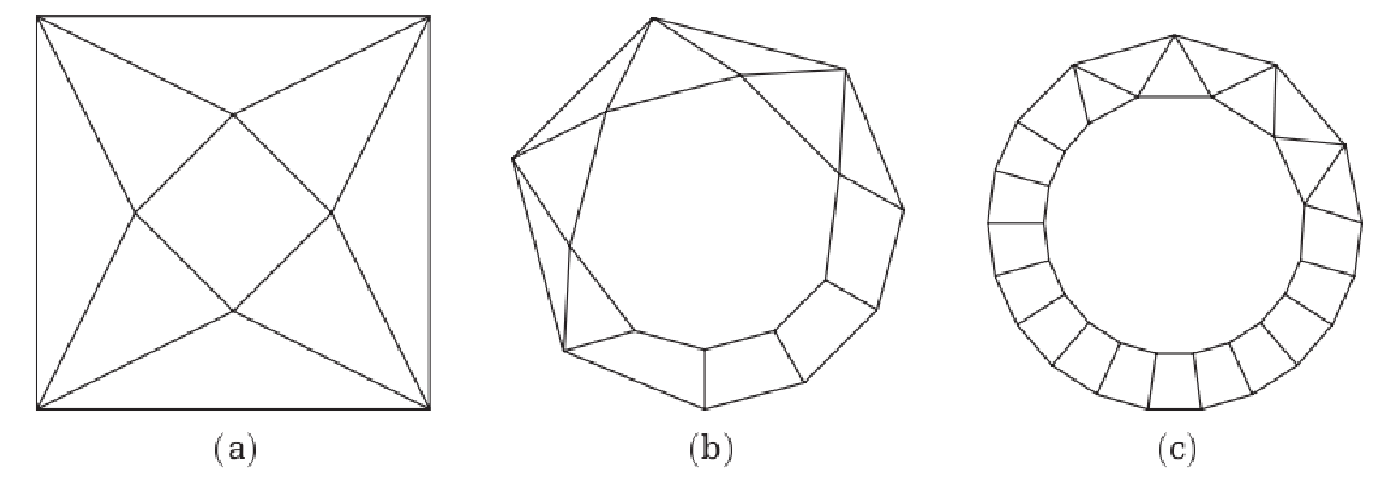
For $g>3$ the graph $\check{\Gamma}$ is given by a ring with 8 triangles next to each other, $2g-6$ quadrilaterals and $4g-4$ vertices, and we shall label its edges as in [2]:

Considering the lifted graph of $\check{\Gamma}$ in the curve $S$ over $\Sigma$, Copeland could show the following in Theorem 16 and Proposition 21 [2]:

Note that $\mathbb{R}[F]\cap\frac{1}{2}\mathbb{Z}[E]$ can be understood by considering the following sum:

Although the summands above are not individually in $\mathbb{R}[F]\cap\frac{1}{2}\mathbb{Z}[E]$, when summed they satisfy

From Proposition 6, the monodromy action for $SL(2,\mathbb{R})$-Higgs bundles can be understood through the monodromy of the Gauss-Manin connection on the mod 2 cohomology of the fibres of the Hitchin fibration. This is the action on $P[2]$, and thus it is convenient to first give a combinatorial description of this space.

Since the space $P[2]$ is given by the quotient of $\mathbb{Z}_{2}[E]$ by the subspace generated by $x_{1},x_{2},x_{4}$ and $x_{5}$, we shall dedicate this section to understand the action of the generators from Theorem 7 on $\mathbb{Z}_{2}[E]$.

For $\Sigma^{[4g-4]}$ be the configuration space of $4g-4$ points in $\Sigma$, there is a natural map $p:\mathcal{A}_{reg}\rightarrow\Sigma^{[4g-4]}$ which takes a quadratic differential to its zero set. Furthermore, $p$ induces the following maps

where $S_{4g-4}$ is the symmetric group of $4g-4$ elements. Thus there is a natural permutation action on $C_{0}$, and Copeland’s generators in $\pi_{1}(\mathcal{A}_{reg})$ map to transpositions in $S_{4g-4}$. Concretely, a generator $\sigma_{e}$ labelled by the edge $e$ as in Theorem 7 acts on another edge $x$ by

where $<\cdot,\cdot>$ is the intersection pairing. As this pairing is skew over $\mathbb{Z}$, for any edge $e$ one has $<e,e>=0$.

We shall give an ordering to the vertices in $\check{\Gamma}$ as in the figure below, and denote by $E^{\prime}\subset E$ the set of dark edges:

The subgroup $S^{\prime}_{4g-4}$ preserves $\mathbb{Z}_{2}[E^{\prime}]$, and the boundary $\partial:C_{1}\rightarrow C_{0}$ is compatible with the action of $S_{4g-4}^{\prime}$ on $C_{1}$ and $S_{4g-4}$ on $C_{0}$. Thus, from Proposition 13, there is a natural homomorphism

which is an isomorphism when restricted to $S^{\prime}_{4g-4}$.

From the above analysis, in terms of $N$ one has that

Any element $g\in G_{1}$ can be expressed uniquely as $g=s\cdot h$, for $h\in N\subset G_{1}$ and $s\in S^{\prime}_{4g-4}\subset G_{1}$. The group action on $C_{1}$ may then be expressed as

for $s_{1},s_{2}\in S_{4g-4}^{\prime}$ and $h_{1},h_{2}\in N$. In order to understand the subgroup $N$ we make the following definition.

Note that each edge $e\in E_{0}$ is contained in only one of such boundaries.

From Proposition 12 the boundaries $\Delta_{e}$ are acted on trivially by $G_{1}$. By comparing the action labelled by the edges in $E_{0}$ with the action of the corresponding transposition in $S^{\prime}_{4g-4}$ one can find out which elements are in $N$.

Then, we have the following possible relations between the action of elements $\sigma_{(i,j)}$ and $s_{(i,j)}$ :

• •

  For a triangle with vertices $i,i+1,i+2$, the generators of $S^{\prime}_{3}\subset S^{\prime}_{4g-4}$ are given by $\sigma_{(i,i+1)}$ and $\sigma_{(i+1,i+2)}$. Then, $(i,i+1),(i+1,i+2)\in E^{\prime}$ and the action labelled by the edge $(i,i+2)\in E_{0}$ can be written as:

  $$s_{(i,i+2)}=\sigma_{(i+1,i+2)}\sigma_{(i,i+1)}\sigma_{(i+1,i+2)}~.$$

• •

  For a square with vertices $i,i+1,i+2,i+3$, the generators of $S^{\prime}_{4}\subset S^{\prime}_{4g-4}$ are given by $\sigma_{(i,i+1)},\sigma_{(i+1,i+2)}$ and $\sigma_{(i+2,i+3)}$. In this case one has that the edges $(i,i+1),(i+1,i+2),(i+2,i+3)\in E^{\prime}$ and the action labelled by the edge $(i,i+3)\in E_{0}$ can be written as:

  $$s_{(i,i+3)}=\sigma_{(i+2,i+3)}\sigma_{(i+1,i+2)}\sigma_{(i,i+1)}\sigma_{(i+1,i+2)}\sigma_{(i+2,i+3)}~.$$

References

- [1] A. Beauville, M.S. Narasimhan and S. Ramanan, Spectral curves and the generalised theta divisor. J. reine angew. Math. 398 (1989), 169-179.
- [2] J. Copeland, Monodromy of the Hitchin map over hyperelliptic curves. IMRN (2005), 1743-1785.
- [3] K. Corlette, Flat -bundles with canonical metrics, J. Differential Geom. 28 (1988), 361-382.
- [4] S.K. Donaldson, Twisted harmonic maps and the self-duality equations, Proc. London Math. Soc. (3) 55 (1987), 127-131.
- [5] O. Garcia-Prada, Involutions of the moduli space of SL(n;C)-Higgs bundles and real forms, In ”Vector Bundles and Low Codimensional Subvarieties: State of the Art and Recent Developments” Quaderni di Matematica, Editors: G. Casnati, F. Catanese and R. Notari (2007).
- [6] W.M. Goldman, Topological components of spaces of representations, Invent. Math. 93 (1988), 557-607.
- [7] P.B. Gothen and A. Oliveira, The singular fibre of the Hitchin map, IMRN (2012).
- [8] N.J. Hitchin, The self-duality equations on a Riemann surface. Proc. LMS 55, 3 (1987), 59-126.
- [9] N.J. Hitchin, Stable bundles and integrable systems, Duke Math. J. 54, 1 (1987), 91-114.
- [10] N.J. Hitchin, Langlands duality and spectral curves, Q.J. Math., 58 (2007), 319-344.
- [11] L.P. Schaposnik, Spectral data for G-Higgs bundles, D. Phil. Thesis, University of Oxford, (2012) arXiv:1301.1981. [math.DG].
- [12] C.T. Simpson, Constructing variations of Hodge structure using Yang-Mills theory and applications to uniformization, Journal of the AMS 1 (1988). 867-918.
- [13] C.T. Simpson, Higgs bundles and local systems, Publ. Math. I.H.E.S. 75 (1992), 5–95.
- [14] K. Walker, Quotient groups of the fundamental groups of certain strata of the moduli space of quadratic differentials. Geometry and Topology, 14 (2010), 1129-1164.