Reconstruction of Gravitational Lensing Using WMAP 7-Year Data

Gravitational lensing of the Cosmic Microwave Background (CMB) provides information on the mass distribution between the surface of last scattering and the observer, thus potentially providing information, for example, on dark energy and neutrino masses. In addition, gravitational lensing causes $E$-modes to be converted into large angular scale $B$-modes, thereby potentially contaminating $B$-mode signature of inflationary gravitational waves [1]. Because lensing deflects CMB photons by approximately $3^{\prime}$, a perturbative treatment to first order is generally valid. An estimator for the deflection angle has been devised by Hu [2, 3].

The first attempt to detect lensing by Hirata et al. [4] used the cross-correlation between the WMAP 1-year data and selected luminous red galaxies (LRGs) from the Sloan Digital Sky Survey (SDSS). No statistically significant signal was found. The first detection of lensing was performed by Smith et al. [5] who used the cross-correlation between the NRAO VLA Sky Survey (NVSS) of radio galaxies with a higher mean redshift than the Sloan LRGs and a fully-optimal lensing estimator on the statistically more powerful WMAP 3-year data. Evidence for lensing was found at the 3.4$\sigma$ level. Using a similar estimator as in [4], Hirata et al. [6] obtained results consistent with, though at slightly lower significance than [5], using WMAP 3-year data, LRGs and quasars from the SDSS data, as well as data from the NVSS. Recently, Smidt et al. [7] used an estimator based upon the kurtosis of the CMB temperature four-point correlation function to estimate lensing from WMAP 7-year data only and claimed evidence for lensing at the $2\sigma$ level. Recently, the Atacama Cosmology Telescope (ACT) collaboration successfully detected gravitational lensing [8] at the 4$\sigma$ level. The South Pole Telescope (SPT) detected the effects of gravitational lensing on the angular power spectrum[9].

In this paper we present a search for gravitational lensing using the WMAP 7-year data alone and the standard optimal quadratic estimator [2, 3] which differs from the kurtosis estimator of [7]. We apply the quadratic estimator to WMAP-7 temperature maps alone for the first time in the hopes that our analysis might serve as a touchstone allowing for consistent comparison between different lensing extraction techniques. We review the notation for full-sky reconstruction of gravitational lensing in Section II. We discuss the sky-cut used in our analysis in Section III. Then we introduce our modified estimator in Section IV making use of the optimal quadratic estimator of [2]. We introduce the WMAP 7-year data in Section V, and describe the details of the calculations, including the noise model, and analysis in Section VI. Results of a null test are shown in Section VII, and we discuss the conclusions of our work in Section VIII.

The effect of lensing on the CMB’s primordial temperature $\tilde{T}$ in direction ${\bf n}$ can be represented by

where $T$ is the lensed temperature and $\mathbf{d}(\mathbf{n})=\mathbf{\nabla}\phi$, with $\phi$ being the lensing potential. The two-point correlation function of the temperature field following [10], is:

where the second term encodes the effects of lensing with the weighting factor $f^{TT}_{lLl^{\prime}}$ given by

Here $\tilde{C}_{l}^{TT}$ are the unlensed temperature power spectra. and

The lensing estimator is constructed from an average over a pair of two-point correlations [2, 3] and has the form

The requirement that the estimator in Eq. (II) is unbiased and has minimal variance results in

and

with $C_{l}^{\rm tot}=C_{l}^{TT}+N_{l}^{TT}$, where $C_{l}^{TT}$ are the lensed power spectra and $N_{l}^{TT}$ is the instrumental noise. In the following, the summations are from $l$ and $l^{\prime}=0$ to 750 and $|m|\leq l$, $|m^{\prime}|\leq l^{\prime}$. The WMAP 7-year data do not contain additional information at higher multipoles.

To reduce computation time we follow [10] and define three maps for the TT estimator:

and take the inverse Spherical Harmonic Transform (SHT) of ${}_{0}A^{T}X$ and ${}_{0}A^{T}Y$ to get

with

Using Eqs. (14), (15) and (16) the expression for $d_{LM}^{TT}$ in Eq. (II) becomes

A similar procedure is followed for the efficient calculation of $A_{L}^{TT}$ in Eq. (12). The resulting expression is given in [11] (originally proposed in [12]):

with the $\xi^{T}$ given by

here $d^{l}_{ss^{\prime}}(\theta)$ are Wigner d-functions.

In order to eliminate contaminated data, regions such as the galactic plane and bright point sources in the full-sky map must be removed using a mask, thereby introducing a sky-cut. For example, in [6], the Kp2 mask was used to make 84.7% of the sky uncontaminated. In [7], the more conservative KQ75 mask was used to clean artifacts around the galactic plane and point sources.

The sky-cut can be removed as a separate component to get a full-sky map before we process the data. One such technique is the “inpainting” method in which the estimated values of pixels in the map are substituted for those removed by the mask. Perotto et al. have simulated the full sky reconstruction for PLANCK [13]. The full-sky map recovered in this way will bias the lensing reconstruction slightly.

Another method proposed by A. Benoit-Levy [14] apodizes the masked regions of the map and inpaints the masked regions of the map by constrained Gaussian random values of the unlensed temperature. In this way, the sky-cut-induced coupling approximately reduces to a unit matrix. However, for WMAP, we have to remove a big portion of the sky, reducing $f_{\rm sky}$ dramatically to $0.3$. The unbiased estimator could be scaled up by a factor of $1/f_{\rm sky}$, but the signal-to-noise ratio would be reduced significantly. This means the uncertainty of the reconstructed signal would be larger.

As opposed to a separate-component solution, we obtain an all-inclusive lensing reconstruction pipeline, using the built-in filter of the estimator to treat the data without pre-conditioning it. The optimal estimator for the potential based on the maximum likelihood is derived by Hirata [15]. The full inverse variance $({\bf{C}}+{\bf{N}})^{-1}$, instead of $(C^{TT}_{L}+N^{TT}_{L})^{-1}$, was used by [5] because it is an optimal filter when there are sky-cuts and inhomogeneous noise. The sky-cut generates artifacts in harmonic space, as does lensing. $({\bf{C}}+{\bf{N}})^{-1}$ can be used to filter those modes affected by the sky-cut. However, we do not use this filter because the inversion of $({\bf{C}}+{\bf{N}})$ is computationally challenging [5]; instead we use the estimator Eq. (II) which is identical to the one of [6], and it is an excellent approximation to the maximum likelihood estimator. We note that, while $(C^{TT}_{L}+N^{TT}_{L})^{-1}$ will be suboptimal to a full $({\bf{C}}+{\bf{N}})^{-1}$ filter, it preserves the simplicity and efficiency of the lensing reconstruction procedure.

For WMAP, we modify the estimator slightly to deal with the instruments’ anisotropic temperature noise.

The observed lensed temperature map $\mathbb{T}$ is given by

and likewise the “observed” unlensed temperature map $\tilde{\mathbb{T}}$ is

Here $M(\mathbf{n})$ represents the mask, $B(\mathbf{n},\mathbf{n^{\prime}})$ the beam, and $N(\mathbf{n})$ the noise.

For a pair of maps $\alpha$ and $\beta$, “$TT(\alpha\times\beta)$” denotes the cross-correlation between these two temperature maps. A harmonic mode of the reconstruction including noise is estimated as

following Eq. (II), and a harmonic mode of the Gaussian bias is estimated as

Here $\mathbb{C}$ are the power spectra of the observed lensed temperature, determined from $\langle\mathbb{T}_{lm}\mathbb{T}_{l^{\prime}m^{\prime}}\rangle$. As was done in [8] and [16] we use the same power spectra in Eq. (31) and Eq. (35). In order to deal with the non-uniform noise distribution in the WMAP data, we symmetrize $\mathbbm{d}^{TT(\alpha\times\beta)}_{LM}$ as in [6], denoting the symmetrized cross-correlation “$TT(\alpha\bullet\beta)$” between these two temperature maps,

and

We refer to $C_{L}^{est}=\langle d_{LM}^{\ast}d_{LM}\rangle$ as the reconstruction including noise, and $N_{L}^{(0)}=\langle N_{LM}^{\ast}N_{LM}\rangle$ as the Gaussian bias, with the superscript “$TT(\alpha\bullet\beta)$” omitted. Thus we obtain

following a reasoning similar to the one near the end of Section II.

The two-point correlation of the Gaussian bias estimator is essentially a four-point correlation function of the primordial temperature modes. It should be carefully subtracted since, for a noise-dominated experiment such as WMAP, the Gaussian four-point bias is several orders of magnitude larger than the lensing power spectra. In [8] phase-randomized data maps are used to simulate this Gaussian bias. However, this approach does not work for the present lensing reconstruction since WMAP’s noise is not isotropic. Evidence for this can be seen from the normalization factor $\mathbbm{A}_{L}^{TT(\alpha\times\beta)}$ which is not equal to $N^{(0)TT(\alpha\bullet\beta)}_{L}$ whereas they should be equal for isotropic noise [10]. The normalization factor Eq. (39) only contains the partial contribution coming from the non-isotropic noise while the Gaussian bias squared from Eq. (37) consists of all the correlations generated by the non-isotropic noise, see [17] and [18]. If the phases of the WMAP temperature maps are randomized in order to remove the lensing-induced coupling between modes, it will also remove the strong correlation of the noise. The Gaussian bias calculated in this way will be significantly lower than that from the standard approach [19]. So we have to perform simulations which use the simulated WMAP noise and temperature maps, rather than the randomized WMAP data to get the Gaussian bias term.

The deflection power spectrum is

This estimator is essentially the same as in [8] except that here it is the full-sky version and the noise $\mathbb{N}_{LM}$ is not obtained from the phase-randomized data. We subtract the Gaussian bias for each realization of the estimator, and all the estimated power spectra are averaged to get the binned power spectra $\langle C_{b}^{dd}\rangle$ for the $b$-th bin [16]. The averaged power spectrum in a range of $L$ labeled by the index $b$ is

The statistical uncertainty is given by $\sigma_{b}=[\langle(C_{b}-\bar{C}_{b})^{2}\rangle]^{\frac{1}{2}}$. After the subtraction of the Gaussian bias, there remains the higher order biases, see [8] (where it was called “null bias”), [16], and [20].

We expand $T$ in harmonic space as

see [21]. Here the power $n$ in $\delta^{n}$ denotes the order in $\phi^{n}$. We expand the noise bias as

where the index $n$ in $N^{(n)}$ denotes the order of its dependence upon $[\phi^{2}]^{n}$, excluding terms that contribute to the lensed power spectrum. The four-point function $\langle\mathbbm{d}^{\ast}_{LM}\mathbbm{d}_{LM}\rangle$ contains terms of different order in $\delta^{n}T$. A term of the type $\langle\delta T\delta T\tilde{T}\tilde{T}\rangle$ contributes to $C_{L}^{dd}$ and the first order noise $N^{(1)}_{L}$ while terms of the type $\langle\delta T\delta T\delta T\delta T\rangle$, $\langle\delta^{2}T\delta^{2}T\tilde{T}\tilde{T}\rangle$, $\langle\delta^{2}T\delta T\delta T\tilde{T}\rangle$, and $\langle\delta^{3}T\delta T\tilde{T}\tilde{T}\rangle$ generate the second order noise $N_{L}^{(2)}$. Following [21], the higher order bias term is calculated as the difference between the estimated power spectrum and the sum of its prediction and the lowest order noise (i.e., Gaussian bias): $C_{L}^{est}-(C_{L}^{dd}+N^{(0)}_{L})$, using Monte Carlo simulations.

We study the statistical significance of the detection as follows. Following [6], the reconstructed power spectra $C^{(\textrm{obs})}$ are compared with their theoretical prior $C^{(\textrm{th})}$ by minimizing a $\chi^{2}$ defined as

and varying $\mathcal{C}$. Here $A$ or $B$ label the range in $L$, and $C_{A}$ or $C_{B}$ is the band-power. The covariance matrix $\mathbf{C}$ is calculated from the Monte Carlo simulation as $\mathbf{C}_{AB}=\langle(C^{(\textrm{sim})}_{A}-\bar{C}^{(\textrm{sim})}_{A})(C^{(\textrm{sim})}_{B}-\bar{C}^{(\textrm{sim})}_{B})\rangle$. The best fit $\mathcal{C}$ is obtained by setting the derivative of $\chi^{2}$ to zero:

A non-zero value of $\mathcal{C}$ indicates the presence of lensing. The signficance of a non-zero value can be judged if its variance is known. The variance of $\mathcal{C}$ is given by

and the significance of the detection of lensing is $\mathcal{C}/\Delta\mathcal{C}$.

We show the higher order bias in Figure 1. The higher order bias $N_{L}^{(1)}+N_{L}^{(2)}+...$ is seen to be negative for $L<20$ and positive for $L>170$ and consistent with zero for $20<L<170$ where the amplitude is $-0.42\pm 0.98$ $(0.43\sigma)$, compared to the simulated lensing signal $C_{L}^{dd}$ by using 15 bins with $\Delta L=10$ starting from $L=20$. In Figure 2, the likelihood of the amplitude of the higher order bias limited to the region $20<L<170$ confirms that the bias is consistent with zero. Thus subtraction of the higher order bias is not required as long as we limit $L$ to this region.

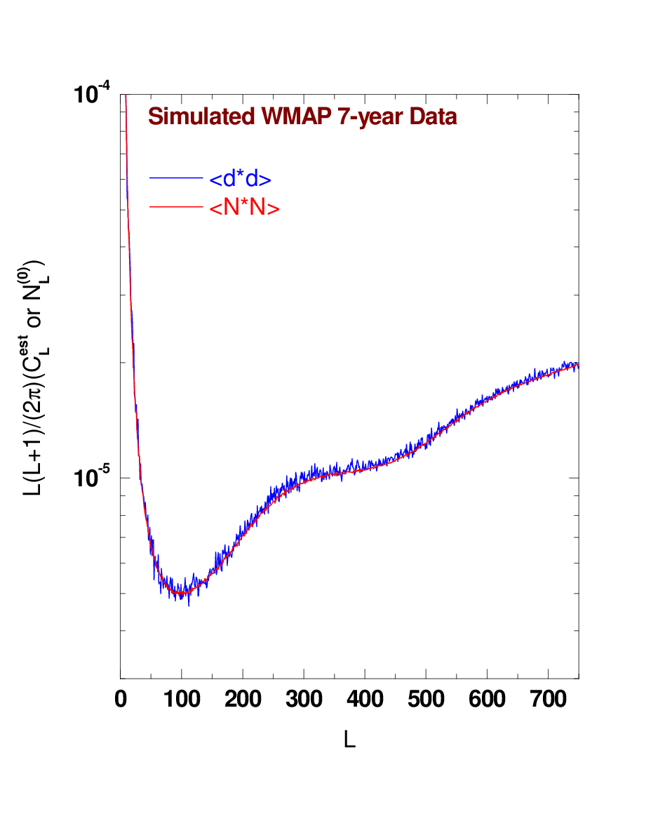
The lensing reconstruction depends most sensitively on the high-$L$ modes which are supplied by WMAP’s DAs in the V (2 DAs) and W (4 DAs) frequency bands. Thus we use WMAP’s coadded temperature maps with r9 resolution (Healpix’s $n_{side}=512$) using all possible distinct pairings: three auto-correlations for the two V-band DAs, ten auto-correlations for the four W-band DAs, and eight cross-correlations between the W- and V-band DAs for a total of 21 correlations (labeled “ALL”). Smith et al. [5], used the Q-band DAs in addition to the W- and V-band DAs of WMAP 3-year temperature maps. Hirata et al. [6], used 153 one-year DAs from the WMAP 3-year data in the W- and V-bands. Recently, Smidt et al. [7] used the W- and V-frequency bands of the WMAP 7-year data. This work adopts six DAs of WMAP’s 7-year temperature map, making the data selection slightly different from other work, although the same signal-to-noise is expected. The WMAP temperature maps contain very high levels of noise as shown in Figure 3. The normalization factor $\mathbb{A}_{L}$ shown in Figure 4 is about two orders of magnitude higher than the signal $C_{L}^{dd}$; indicative of the difficulty of extracting the lensing from the noisy data. We calculate the noise in each band from WMAP’s data instead of using an analytical form as [4] and [6] do. The noise is simulated according to the prescription in [19], and the beam transfer functions are supplied by WMAP.

We use the CAMB code [22] to obtain the power spectra $\tilde{C}_{l}^{TT}$, and $C_{l}^{\phi\phi}$ using a six parameter $\Lambda$CDM model with $\textbf{P}={\omega_{b}h^{2},\omega_{c}h^{2},h,\tau,A_{s},n_{s}}={0.0226,0.112,0.70,0.09,2.1\times 10^{-9},0.96}$. These are input into a pipeline that has elements as follows.

Gaussian maps of the deflection angle field $\mathbf{d}(\mathbf{n})$ and unlensed temperature $\tilde{T}(\mathbf{n})$ are generated using their respective power spectra. We use $\tilde{C}_{l}^{TT}$, and $C_{l}^{\phi\phi}$ to create one realization of the simulated deflection field and lensed temperature maps $T(\mathbf{n})$ are generated using Eq. (1) with the $\tilde{T}(\mathbf{n})$ and $\mathbf{d}(\mathbf{n})$ found above.

Using the inverse SHT, the temperature maps are converted into harmonic modes $a_{lm}$ which are convolved with the beam transfer functions $b_{l}$. Using SHT, these are transformed into configuration space and WMAP-based noise is added. We mask the galactic plane and point sources using WMAP’s KQ75 mask. Using inverse SHT, the resulting maps are transformed back into harmonic space where new $a_{lm}$ are kept up to $l_{max}=750$ and $|m_{max}|=750$.

The noise simulation is crucial to this work because the $N^{(0)}_{L}$ is one hundred times larger than $C_{L}^{dd}$. The six V- and W-band DAs, labeled by $\alpha=V1$, $V2$, $W1$, $W2$, $W3$, $W4$, have different noise variances, different beam transfer functions, and different relative phases. To mimic the WMAP DAs, we simulate the Gaussian bias as follows. Using

we set the index $i$ (an arbitrary running index) for Eq. (47) and generate an unlensed temperature map $\tilde{T}^{(i)}(\mathbf{n})$, and six noise maps $N^{(i)\alpha}({\bf n})$, $\alpha=V1$, $V2$, $W1$, $W2$, $W3$, $W4$. Then we make an observed map $\tilde{\mathbb{T}}^{(i)\alpha}(\mathbf{n})$ using Eq. (47), and repeat this procedure to make another observed map $\tilde{\mathbb{T}}^{(i)\beta}(\mathbf{n})$. Subsequently, we calculate the Gaussian bias $N^{(0)}_{L}$ using Eq. (37) for the pair $(\alpha\bullet\beta)$. In the same way, we generate 21 realizations for all the correlations. Finally we increase the index $i$, and repeat the whole procedure until the ensemble $\{N^{(0)}_{L}\}$ has 700 elements.

We proceed in a similar manner simulating the reconstruction including noise, except setting $T^{(i)}({\bf n})=T({\bf n})$ and $N^{(i)\alpha}(\mathbf{n})=N^{\alpha}(\mathbf{n})$. Using

we set the index $i$ for Eq. (48), and generate a lensed temperature map $T^{(i)}(\mathbf{n})$, and six noise maps $N^{(i)\alpha}({\bf n})$, $\alpha=V1$, $V2$, $W1$, $W2$, $W3$, $W4$. Then we make an observed map $\mathbb{T}^{(i)\alpha}(\mathbf{n})$ using Eq. (48) and repeat this procedure to make another observed map $\mathbb{T}^{(i)\beta}(\mathbf{n})$. Subsequently we calculate the reconstruction including noise $C^{est}_{L}$ using Eq. (36) for the pair $(\alpha\bullet\beta)$. In the same way, we generate 21 realizations for all the correlations. Finally we increase the index $i$, and repeat the whole procedure until the ensemble $\{C^{est}_{L}\}$ has 700 elements. Eq. (40) is then used to obtain the deflection power spectrum $C_{L}^{dd}$.

We show the reconstruction including noise $C_{L}^{est}$ and the Gaussian bias $N_{L}^{(0)}$ in Figures 5, and 6 for the real and the simulated WMAP data, respectively. The simulation is consistent with the data, and we confirm that the two terms in Eq. (40) nearly have the same magnitude, and the lensing induced difference is not visible because the lensing signal $C_{L}^{dd}$ is one hundred times smaller than the Gaussian bias $N_{L}^{(0)}$. We use Eq. (40) to calculate the reconstructed lensing power spectra in Figure 7.

The likelihood distribution of $\mathcal{C}$ is shown in Figure 8, where it is seen lensing is detected at only 1.30$\sigma$ confidence level.

To check for systematic effects, we employ the “curl null test”. The deflection angle field can be written as the sum of a gradient and a curl term [23]:

The first term leads to the Hu estimator [2, 3]

whose efficient form is given in Eq. (38), here ${}_{0}A^{T}({\bf{n}})$ is given by Eq. (14) and

The estimator for the curl part in Eq. (49) is

and the corresponding efficient form is

which can be compared with Eq. (38). We show the resulting power spectra $C_{L}^{\delta\delta}$, averaged from 700 realizations from the real and the simulated WMAP data separately in Figure 9. The averaged curl component amplitude is $0.38\pm 0.79$ consistent with zero as expected, compared to the simulated $C_{L}^{dd}$.

In this work, we have applied the optimal quadratic estimator to WMAP-7 temperature maps alone for the first time.

We have monitored the convergence behavior for the mean value $\mathcal{C}$, the error $\Delta\mathcal{C}$, and the detection significance $\mathcal{C}/\Delta\mathcal{C}$ of the reconstructed lensing signal $C_{L}^{dd}$. We find that all these quantities converge after producing 700 realizations of the reconstructed lensing signal, see Figure 10. We determine the significance of the lensing detection and find $\mathcal{C}=1.27\pm 0.98$ $(1.30\sigma)$, while Smidt et al. found $\mathcal{C}=0.97\pm 0.47$ $(2.06\sigma)$. The result is shown in Table 1 as well as a comparison with [4, 6, 5, 8, 7, 9]. All our results have been corrected by the sky fraction. We find evidence for lensing only at $1.30\sigma$, using all correlations of WMAP-7’s W- and V-band DAs. The resulting constraint on the lensing amplitude differs from [7] and this can be explicated from several aspects. In terms of the estimator, we use the optimal estimator derived from minimum variance principle [2], rather than the kurtosis estimator in [7]. We adopt the individual beam transfer function associated with each DA, not the averaged one for each frequency. We have taken into account the impact of the higher order bias, afterwards restricting the reconstruction in a proper multiple range that marginally overlaps with [7]. In terms of the noise model, we estimate the noise in a way which mimics WMAP, not simply generating random underlying skies and associated noises with independent phases. All these factors may jointly contribute to the difference between us and Smidt et al. A summary of various tests in this work is shown in Table 2. We do not observe a significant lensing signal from the WMAP 7-year temperature data.

We did not apply a correction for higher order bias terms $N^{(1)}_{L}$, $N^{(2)}_{L}$, …, because they are expected to be small owing to the fact that we limited the region of $L$ to $20<L<170$, where the higher order bias is consistent with zero. The higher order bias can be obtained via an iterative solution[18] but it is computationally demanding and not warranted in the present case because we do not obtain a significant signal.

We applied the curl null test to all the correlations of W- and V-band DAs as a systematic check, since we observe a small amount of power from the reconstructed gravitational lensing signal (Figure 7). The reconstruction procedure passes the curl null test.

The effects of beam systematics and the galactic and foreground contaminations are quite small compared to the statistical error. We do not correct the statistical result for the presence of point sources because they introduce negligible systematics [19].

We have demonstrated, using a nearly optimal estimator, that WMAP-7 data does not have the power to detect gravitational lensing, which is unfortunate since WMAP data is the only publicly available data set with sufficient angular resolution to detect lensing. However, WMAP-7 does have value as a publicly available tool to assess the efficacy of lensing algorithms and to test for systematic biases.