Magnetic helicity fluxes and their effect on stellar dynamos

The magnetic field of the Sun and other astrophysical objects, like galaxies, show field strengths that are close to equipartition and length scales that are much larger than that of the underlying turbulent eddies. Their magnetic field is assumed to be generated by a turbulent dynamo. Heat is transformed into kinetic energy, which then generates magnetic energy, which reaches values close to the kinetic energy, i.e. they are in equipartition. The central question in dynamo theory is under which circumstances strong large-scale magnetic fields occur and what the mechanisms behind it are.

During the dynamo process, large- and small-scale magnetic helicities of opposite signs are created. The presence of small-scale helicity works against the kinetic $\alpha$-effect, which drives the dynamo (Pouquet et al.,, 1976; Brandenburg,, 2001; Field & Blackman,, 2002). As a consequence, the dynamo saturates on resistive timescales (in the case of a periodic domain) and to magnetic field strengths well below equipartition (in a closed domain). This behavior becomes more pronounced with increasing magnetic Reynolds number $\mbox{\rm Re}_{\rm M}$, such that the saturation magnetic energy of the large-scale field decreases with $\mbox{\rm Re}_{\rm M}^{-1}$ (Brandenburg & Subramanian,, 2005), for which it is called catastrophic. Such concerns were first pointed out by Vainshtein & Cattaneo, (1992). The quenching is particularly troublesome for astrophysical objects, since for the Sun $\mbox{\rm Re}_{\rm M}=10^{9}$ and galaxies $\mbox{\rm Re}_{\rm M}=10^{18}$.

The first part of this work addresses if fluxes of small-scale magnetic helicity in an $\alpha^{2}$ dynamo can alleviate the catastrophic quenching. We want to reach as high magnetic Reynolds numbers as possible. Consequently we consider the mean-field formalism (Moffatt,, 1980; Krause & Rädler,, 1980) in one dimension, where a field $\textstyle B$ is split into a mean part $\overline{\bm{B}}$ and a fluctuating part $\textstyle b$. In mean-field theory the induction equation reads

with the mean magnetic field $\overline{\bm{B}}$, the mean velocity field $\overline{\bm{U}}$, the magnetic diffusivity $\eta$, and the electromotive force $\overline{\mbox{\boldmath${\cal E}$}}{}=\overline{\mathchoice{\mbox{\boldmath$\displaystyle u$}}{\mbox{\boldmath$\textstyle u$}}{\mbox{\boldmath$\scriptstyle u$}}{\mbox{\boldmath$\scriptscriptstyle u$}}{}\times\mathchoice{\mbox{\boldmath$\displaystyle b$}}{\mbox{\boldmath$\textstyle b$}}{\mbox{\boldmath$\scriptstyle b$}}{\mbox{\boldmath$\scriptscriptstyle b$}}{}}$, where $\mathchoice{\mbox{\boldmath$\displaystyle u$}}{\mbox{\boldmath$\textstyle u$}}{\mbox{\boldmath$\scriptstyle u$}}{\mbox{\boldmath$\scriptscriptstyle u$}}{}=\mathchoice{\mbox{\boldmath$\displaystyle U$}}{\mbox{\boldmath$\textstyle U$}}{\mbox{\boldmath$\scriptstyle U$}}{\mbox{\boldmath$\scriptscriptstyle U$}}{}-\overline{\bm{U}}$ and $\mathchoice{\mbox{\boldmath$\displaystyle b$}}{\mbox{\boldmath$\textstyle b$}}{\mbox{\boldmath$\scriptstyle b$}}{\mbox{\boldmath$\scriptscriptstyle b$}}{}=\mathchoice{\mbox{\boldmath$\displaystyle B$}}{\mbox{\boldmath$\textstyle B$}}{\mbox{\boldmath$\scriptstyle B$}}{\mbox{\boldmath$\scriptscriptstyle B$}}{}-\overline{\bm{B}}$ are fluctuations. A common approximation for $\overline{\mbox{\boldmath${\cal E}$}}{}$, which relates small-scale with the large-scale fields, is

where $\eta_{\rm t}=u_{\rm rms}/(3k_{\rm f})$ is the turbulent magnetic diffusivity in terms of the rms velocity $u_{\rm rms}$ and the wavenumber $k_{\rm f}$ of the energy-carrying eddies, and $\alpha$ = $\alpha_{\rm K}+\alpha_{\rm M}$ is the sum of kinetic and magnetic $\alpha$, respectively. The kinetic $\alpha$ is the forcing term, i.e. the energy input to the system. In this model $\alpha_{\rm K}$ vanishes at the mid-plane and grows approximately linearly with height until it rapidly falls off to $0$ at the boundary. The magnetic $\alpha$ can be approximated by the magnetic helicity in the fluctuating fields: $\alpha_{\rm M}\approx\overline{h}_{\rm f}\times(\mu_{0}\rho_{0}\eta_{\rm t}k_{\rm f}^{2}/B_{\rm eq}^{2})$, where $\mu_{0}$ is the vacuum permeability, $\rho_{0}$ is the mean density, $B_{\rm eq}=(\mu_{0}\rho_{0})^{1/2}u_{\rm rms}$ is the equipartition field strength and $\overline{h}_{\rm f}=\overline{\mathchoice{\mbox{\boldmath$\displaystyle a$}}{\mbox{\boldmath$\textstyle a$}}{\mbox{\boldmath$\scriptstyle a$}}{\mbox{\boldmath$\scriptscriptstyle a$}}{}\cdot\mathchoice{\mbox{\boldmath$\displaystyle b$}}{\mbox{\boldmath$\textstyle b$}}{\mbox{\boldmath$\scriptstyle b$}}{\mbox{\boldmath$\scriptscriptstyle b$}}{}}$ the magnetic helicity in the large-scale fields.

The advantage of this approach is that we can use the time evolution equation for the magnetic helicity to obtain the evolution equation for the magnetic $\alpha$ (Brandenburg et. al.,, 2009)

where $\overline{\mbox{\boldmath${\cal F}$}}{}_{\alpha}$ is the magnetic helicity flux term. To distinguish this from the algebraic quenching (Vainshtein & Cattaneo,, 1992) it is called dynamical $\alpha$-quenching.

For the flux term on the RHS of equation (3) we either choose it to be diffusive, i.e. $\overline{\mbox{\boldmath${\cal F}$}}{}_{\alpha}=-\kappa_{\alpha}\mathchoice{\mbox{\boldmath$\displaystyle\nabla$}}{\mbox{\boldmath$\textstyle\nabla$}}{\mbox{\boldmath$\scriptstyle\nabla$}}{\mbox{\boldmath$\scriptscriptstyle\nabla$}}{}\alpha_{\rm M}$, or we take it to be proportional to $\overline{\mbox{\boldmath${\cal E}$}}{}\times\overline{\mbox{\boldmath$A$}}$, where $\overline{\mbox{\boldmath$A$}}$ is the vector potential of the mean field $\overline{\bm{B}}=\mathchoice{\mbox{\boldmath$\displaystyle\nabla$}}{\mbox{\boldmath$\textstyle\nabla$}}{\mbox{\boldmath$\scriptstyle\nabla$}}{\mbox{\boldmath$\scriptscriptstyle\nabla$}}{}\times\overline{\mbox{\boldmath$A$}}$. The latter expression follows from the recent realization (Hubbard & Brandenburg,, 2011) that terms involving $\overline{\mbox{\boldmath${\cal E}$}}{}$ should not occur in the expression for the flux of the total magnetic helicity. This will be referred to as the alternate quenching model.

Without diffusive magnetic helicity fluxes ($\kappa_{\alpha}=0$), quenching is not alleviated and the equilibrium magnetic energy decreases as $\mbox{\rm Re}_{\rm M}^{-1}$ (Fig. 1). We find that diffusive magnetic helicity fluxes through the mid-plane can alleviate the catastrophic $\alpha$ quenching and allow for magnetic field strengths close to equipartition. The diffusive fluxes ensure that magnetic helicity of the small-scale field is moved from one half of the domain to the other where it has opposite sign. With the alternate quenching formalism we obtain larger values than with the usual dynamical $\alpha$-quenching–even without the diffusive flux term. The magnetic energies are however higher than expected from simulations (Brandenburg & Subramanian,, 2005; Hubbard & Brandenburg,, 2011), which raises questions about the accuracy of the model or its implementation.

In this second part we address the implications arising from adding shear to the system and study the symmetry properties of the magnetic field in a full domain. The large scale velocity field in equation (1) is then $\overline{\bm{U}}=(0,Sz,0)$, where $S$ is the shearing amplitude and $z$ the spatial coordinate. We normalize the forcing amplitude $\alpha_{0}$ and the shearing amplitude $S$ conveniently:

with the smallest wave vector $k_{1}$.

First we perform runs for the upper half of the domain using closed (perfect conductor or PC) and open (vertical field or VF) boundaries and impose either a symmetric or an antisymmetric mode for the magnetic field by adjusting the boundary condition at the mid-plane. A helical forcing is applied, which increases linearly from the mid-plane. The critical values for the forcing and the shear parameter for which dynamo action occurs are shown in Fig. 2.

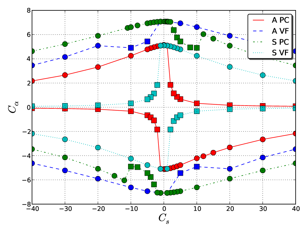
Imposing the parity of the magnetic field is however unsatisfactory, since it a priori excludes mixed modes. Accordingly we compute the evolution of full domain systems with closed boundaries and follow the evolution of the parity of the magnetic field. The parity is defined such that it is 1 for a symmetric magnetic field and $-1$ for an antisymmetric one:

with the domain height $H$. In direct numerical simulations $B_{x}(z)$ and $B_{y}(z)$ are horizontal averages. The field reaches an antisymmetric solution after some resistive time $t_{\rm res}=1/(\eta k_{1}^{2})$ (Fig. 4), which depends on the forcing amplitude $C_{\alpha}$. To check whether symmetric modes can be stable, a symmetric initial field is imposed. This however evolves into a symmetric field too (Fig. 4), from which we conclude that it is the stable mode.

The mean-field results are tested in 3-D direct numerical simulations (DNS); Figs. 6 and 6. The behavior is similar to the mean-field results. The preferred mode is always the antisymmetric one and the time for flipping increases with the forcing amplitude $C_{\alpha}$. This is however very preliminary work and has to be studied in more detail.

The present work has shown that the magnetic helicity flux divergences within the domain are able to alleviate catastrophic quenching. This is also true for the fluxes implied by the alternate dynamical quenching model of Hubbard & Brandenburg, (2011). However, those results deserve further numerical verification. Further, we have shown that, for the model with magnetic helicity fluxes through the mid-plane, the preferred mode is indeed dipolar, i.e. of odd parity. Here, both mean-field models and DNS are found to be in agreement.

References

- Brandenburg, (2001) Brandenburg, A. 2001, ApJ, 550, 824
- Brandenburg et. al., (2009) Brandenburg, A., Candelaresi, S. & Chatterjee, P. 2009, MNRAS, 398, 1414
- Brandenburg & Subramanian, (2005) Brandenburg, A. & Subramanian, K. 2005, Astron. Nachr., 326, 400
- Field & Blackman, (2002) Field, G. B. & Blackman, E. G. 2002, ApJ, 572, 685
- Hubbard & Brandenburg, (2011) Hubbard, A. & Brandenburg, A. 2011, ApJ, in press, arXiv:1107.0238
- Krause & Rädler, (1980) Krause, F. & Rädler, K.-H., Mean-field Magnetohydrodynamics and Dynamo Theory. Oxford: Pergamon Press (1980).
- Moffatt, (1980) Moffatt, H. K., Magnetic Field Generation in Electrically Conducting Fluids. Cambridge: Cambridge Univ. Press (1978).
- Pouquet et al., (1976) Pouquet, A., Frisch, U. & Leorat, J. 1976, J. Fluid Mech., 77, 321
- Vainshtein & Cattaneo, (1992) Vainshtein, S. I., & Cattaneo, F. 1992, ApJ, 393, 165
Sacha BrunIs there a reason that your system prefers antisymmetric solutions? It seems linked to your choice of parameters.
Simon CandelaresiSo far we do not see a reason for that. But we see a parameter dependence of the transition time. We will look at the growth rate of the modes independence of the parameters. This will give us some better clue if also mixed or symmetric modes are preferred.
Gustavo GuerreroIs there a regime where the advective flux removes all the mean field out of the domain?
Simon CandelaresiIf the advective flux is too high the magnetic field gets shed before it is enhanced, which kills the dynamo. So, there is a window for the advection strength for which it is beneficial for the dynamo.