Cluster Density Profiles as a Test of Modified Gravity

In $f(R)$ gravity, the Einstein-Hilbert action is supplemented by a free function of the Ricci scalar $R$,

Here, $\mathcal{L}_{\rm m}$ is the matter Lagrangian and we have set $c=1$. Variation with respect to the metric $g_{\mu\nu}$ yields the modified Einstein equations for metric $f(R)$ gravity,

where the connection is of Levi-Civita type and $f_{R}\equiv\mathrm{d}f/\mathrm{d}R$ is the additional scalar degree of freedom of the model, characterizing the force modifications.

We specialize our considerations to the functional form [34]

where $m^{2}\equiv 8\pi\,G\,\bar{\rho}_{\rm m}/3$. The free parameters of the model $c_{1}$, $c_{2}$, and $n$ can be chosen to reproduce the $\Lambda$CDM expansion history and satisfy solar-system tests [34] through the chameleon mechanism [31, 32, 33]. In the high-curvature regime, $c_{2}^{1/n}R\gg m^{2}$, Eq. (3) simplifies to

where $\bar{R}_{0}$ denotes the background curvature today, $\bar{R}_{0}=\bar{R}|_{z=0}$ , and $f_{R0}\equiv f_{R}(\bar{R}_{0})$. We further infer

from requiring equivalence with $\Lambda$CDM when $|f_{R0}|\rightarrow 0$ and restrict to models with $n=1$. Varying $n$ changes the evolution of the Compton wavelength of the $f_{R}$ field with redshift. Generally, constraints on $f_{R0}$ become weaker (stronger) for $n>1$ ($n<1$) (see [52] for a study of the mass function of halos in $f(R)$ with varying $n$). In the following, we will further assume that $|f_{R0}|\ll 1$, and drop terms that are higher order in $f_{R}$.

In the quasistatic limit, the trace and time-time component of the modified Einstein equations yield the $f_{R}$ field equation and Poisson equation for the Newtonian potential $\Psi=\delta g_{00}/(2g_{00})$ in the longitudinal gauge. Specifically,

Here, coordinates are comoving, $\delta f_{R}=f_{R}(R)-f_{R}(\bar{R})$, $\delta R=R-\bar{R}$, $\delta\rho_{\rm m}=\rho_{\rm m}-\bar{\rho}_{\rm m}$. In contrast, the potential $\Psi_{-}\equiv(\Psi-\Phi)/2$, where $\Phi=\delta g_{ii}/(2g_{ii})$, governing the propagation of light and hence lensing is only affected at order $f_{R}$, which is of order $10^{-2}$ or less for the models we consider here. Hence, the modifications to cluster-galaxy lensing studied in this paper are caused by modifications in the distribution of matter, which arise from the enhanced gravitational forces.

If the background field $|f_{R0}|$ is large compared to typical gravitational potentials ($\sim 10^{-5}$), we may linearize the field equations via the approximation

where $\lambda_{\rm C}=1/m_{f_{R}}$ is the Compton wavelength of the field at the background. In Fourier space, the solution to Eqs. (6) and (7) within the linearized approximation is

where $k=|{\bf k}|$. For scales $k\gg 2\pi\,\lambda_{\rm C}^{-1}a$, this leads to an enhancement of gravitational forces by a factor of $4/3$. Computations using Eq. (9) are referred to as the no-chameleon or linearized $f(R)$ case [49].

If the background field becomes small compared to the depth of the gravitational potential of the object considered ($|f_{R0}|\lesssim 10^{-5}$, small-field limit), the chameleon mechanism becomes active, suppressing non-Newtonian forces. More precisely, $\delta f_{R}\approx-\overline{f_{R}}$ and from Eq. (6), $\delta R\simeq 8\pi\,G\,\delta\rho_{\rm m}$, which restores the standard Poisson equation in Eq. (7). Given that the constraints on $|f_{R0}|$ expected from our lensing data are well within the large-field regime ($|f_{R0}|\gg 10^{-5}$), we can apply the approximation Eq. (9) in the simulations.

Weak gravitational lensing serves as a powerful probe of the total matter distribution (baryonic + dark matter) within our Universe. Here, we focus on stacked cluster-galaxy lensing, which measures the average deformation of background galaxy images around foreground maxBCG galaxy clusters. By averaging over many lenses, the contribution of unassociated large-scale structure is suppressed.

We use the tangential shear $\gamma_{t}$ , measured using the ellipticities of galaxy shapes, as a function of the comoving transverse separation from the lens $r_{\perp,{\rm l}}\approx\theta\left(1+z_{\rm l}\right)D_{\rm l}$. Here, $D_{\rm l}$ is the angular diameter distance to the lens and $z_{\rm l}$ is the lens redshift. After stacking many clusters, the mass distribution becomes symmetric around the line of sight. Then, the shear is related to the excess surface mass density around the dark matter halos hosting the clusters, $\Delta\Sigma(r_{\perp})$, through [53]

The excess surface mass density is related to the projected surface density $\Sigma(r_{\perp})$ through

Here and throughout the paper, $r$ denotes a three-dimensional separation, while $r_{\perp}$ refers to a projected two-dimensional separation. The comoving critical surface mass density is given by

where $D_{\rm s}$ and $D_{\rm ls}$ denote the angular diameter distance to the source and between the lens and the source, respectively. Note that both $\Sigma_{\rm crit}$ and the conversion between $\theta$ and $r_{\perp}$ are dependent on the specific cosmological model (see §VI.3).

Assuming perfect centering of the lenses, the projected surface mass density is related to the halo profiles by

where $H$ indicates the Hubble parameter, $\chi_{l}$ denotes the comoving distance to the lens, and $y$ denotes the distance from the lens along the line of sight. $\xi_{\rm hm}(r)$ is the halo-matter correlation function which quantifies the total mass distribution around halo centers (see §III.3). The lensing window $g_{\rm l}(\chi)$ depends on the source redshift distribution $p_{\rm s}(\chi)$ as

assuming that $p_{\rm s}(\chi)$ is normalized to integrate to unity. The halo-matter correlation function decays strongly with increasing separation, so for the transverse scales considered in this study, the lensing strength $g_{\rm l}(\chi)$ is effectively a constant.

Since our constraints lie in a regime where the chameleon mechanism is not active and we require sufficient halo statistics, we employ no-chameleon $f(R)$ gravity simulations, which solve the linearized $f_{R}$ field equation, Eq. (9) [48, 49, 36]. Simulations are conducted for $|f_{R0}|=10^{-2},\ 10^{-3},\ 10^{-4},\ 0$ and $n=1$. Note that $|f_{R0}|=0$ corresponds to $\Lambda$CDM. Other cosmological parameters are fixed to values following the WMAP 3-year results, $\Omega_{\Lambda}=0.76$, $\Omega_{\rm b}=0.04181$, $h=0.73$, $n_{\rm s}=0.958$, and the initial power in curvature fluctuations $A_{\rm s}=(4.89\times 10^{-5})^{2}$ at $k=0.05~\textrm{Mpc}^{-1}$, corresponding to $\sigma_{8}=0.82$ at $z=0$. The simulations are carried out on $512^{3}$ grid cells with a total of $N_{\rm p}=256^{3}$ particles. Due to the limited volume and resolution of the $f(R)$ simulations, we combine results from two different box sizes, $L_{\rm box}=64h^{-1}~\text{Mpc},\ 128h^{-1}~\text{Mpc}$. Only the smaller boxes contribute for $r<0.75h^{-1}~\text{Mpc}$, corresponding to 3 grid cells for $L_{\rm box}=128h^{-1}~\text{Mpc}$. The box sizes and number of runs for each value of $|f_{R0}|$ are summarized in Table 1.

Halos within the simulation and their associated masses are identified via a spherical overdensity (SO) algorithm (cf. [55]). The particles are placed on the grid by a cloud-in-cell interpolation and counted within a growing sphere around the center of mass until the required overdensity is reached. The mass of the halo is then defined by the sum of the particle masses contained in the sphere. This process is started at the highest overdensity grid point and hierarchically continued to lower overdensity grid points until all halos are identified. The halos employed for this analysis ($\log_{10}M\gtrsim 10^{14}h^{-1}~M_{\odot}$) generally contain more than $10^{3}$ particles.

The zhorizon simulations comprise $30+24$ pure dissipationless dark matter $N$-body simulations of different $\Lambda$CDM cosmologies (see Table 2), designed for high-precision studies of cosmological structures on scales of up to a few $100h^{-1}~\text{Mpc}$ [54, 58].

The matter density field is sampled by $N_{\rm p}=750^{3}$ dark matter particles of mass $M_{\rm dm}=5.55\times 10^{11}h^{-1}~M_{\odot}$, in the fiducial case, with a box size of $1.5h^{-1}~\text{Gpc}$. For the nonlinear gravitational evolution of the equal-mass particles, the publicly available gadget-2 code [59] is used. In order to avoid two-particle collisions, a force softening length of $60h^{-1}~\textrm{kpc}$ is employed. The transfer function at redshift $z=0$ is generated using cmbfast [60] and then rescaled to the initial redshift $z_{\rm i}=50$, where a realization of the potential on the grid is calculated. The particles are placed on a Cartesian grid of spacing $\Delta x=2h^{-1}~\text{Mpc}$ and then displaced according to second-order Lagrangian perturbation theory using the 2lpt code [61, 62].

For each cosmology, we use four boxes from the zhorizon simulations, yielding an effective volume of $13.5h^{-3}~\textrm{Gpc}^{3}$. For all snapshots of each simulation, gravitationally bound structures are identified by a Friends-of-Friends (FoF) algorithm [63] with linking length of 0.2 times the mean interparticle spacing ¹¹ 1 The FoF code used (b-fof) was kindly provided by V. Springel.. The halo center is associated with the minimum of the potential of the particle distribution. Halos with fewer than 20 particles are rejected, resulting in a halo-mass resolution of $M>1.2\times 10^{13}~h^{-1}~M_{\odot}$, corresponding to a halo-number density $\bar{n}=3.7\times 10^{-4}h^{-3}~\text{Mpc}^{3}$.

Cluster-galaxy lensing measures a projection of the halo-matter cross correlation $\xi_{\rm hm}(r)$. We measure $\xi_{\rm hm}$ by averaging the spherically averaged density distribution around halos in the $\Lambda$CDM and $f(R)$ simulations:

In observations, clusters are selected according to their optical richness. The true mass can, however, deviate from the mass inferred from the mass-richness relation [64]. Thus, it is important to take into account the scatter in the mass-richness relation. In the simulations, we model the scatter by a log-normal distribution, assigning a new mass to each halo in the simulations by

where $M_{0}$ is the true mass and $\mathcal{N}$ is the normal distribution with zero mean and variance $\sigma^{2}$. The scatter $\sigma$ is left as a free parameter in the likelihood analysis. We apply this scatter, with $\sigma=0,0.4,0.6,0.8$, to the halo masses in the simulations, then we mass order the halos according to the simulated mass with scatter, and finally select the $N_{\text{h}}$ most massive ones until the required cluster abundance $\bar{n}$ is achieved. Here, $\bar{n}$ is the estimated true average number density of the maxBCG sample (see §V). Specifically, we require $N_{\rm h}=\bar{n}\,V_{\rm tot}$ at $z=0.23$, the mean redshift of the lens sample (see §V), where $V_{\rm tot}$ is the simulation volume. In the following, we will denote the corresponding mass profile as $\xi_{\rm hm}^{\Lambda\rm CDM}$. The same procedure is applied to the $f(R)$ simulations at $z=0.22$, but only for values of $\sigma=0,0.6$ for the scatter.

As discussed in §V, a cylindrical cut is applied to the observational data in order to remove satellite galaxies. In the data this procedure removes both true clusters and satellite galaxies. To account for the removal of clusters, we mimic this approach in the zhorizon simulation analysis, following the same algorithm and using $\delta\chi=\pm 100h^{-1}~\text{Mpc}$ for the length of the cylinder. This reduces the number density by 20% from $\bar{n}=1.8\times 10^{-5}h^{-3}~\text{Mpc}^{3}$ to $\bar{n}=1.45\times 10^{-5}h^{-3}~\text{Mpc}^{3}$ for zero scatter and to $\bar{n}=1.43\times 10^{-5}h^{-3}~\text{Mpc}^{3}$ for scatter $\sigma=0.4$. Since the simulations contain only true halo centers, we conclude that $2/3$ of the 30% of the maxBCG sample removed from the data were true clusters and $1/3$ were contaminating satellite galaxies. After applying the cylindrical cuts, the abundances of halos in the simulation and maxBCGs in the data sample agree very well.

Since the $f(R)$ simulations are of worse resolution and smaller volume compared to the $\Lambda$CDM simulations, we parametrize the relative effect on the halo-matter cross correlation $\xi_{\rm hm}$, rather than $\xi_{\rm hm}$ itself. That is, we measure

from the simulation outputs at $z=0.22$ with $|f_{R0}|>0$ and $|f_{R0}|=0$. We apply the scatter in mass as is done in the $\Lambda$CDM simulations (but only for $\sigma=0,\,0.6$). In order to compare the $f(R)$ gravity profiles to their $\Lambda$CDM counterparts, we consider two cases: a fixed common lower mass limit $M_{0}$, derived from the $\Lambda$CDM concordance cosmology (threshold-matched case, TM); and a lower mass limit for $f(R)$ adjusted to match the abundance of tracers $\bar{n}$ (abundance-matched case, AM). Since the mass function of halos is enhanced in $f(R)$ gravity, the $f(R)$ mass threshold is higher in the second case. The AM case is a consistent approach for comparing $f(R)$ gravity to $\Lambda$CDM; on the other hand, in the TM approach, we purely rely on the modified gravity effects on halo profiles, without explicitly using the information from the mass function that has been used to place constraints on $f(R)$ in [7].

The effects of a modification of gravity are significantly less severe in the TM case as compared to the abundance-matched case, i.e., when taking into account that massive halos are more abundant in $f(R)$. This effect is illustrated in Fig. 1, which shows $\mathcal{Q}_{\rm sim}(r)$ normalized to unity at the peak, i.e., $g(r)$ [see Eq. (18)], and Fig. 2, which shows the peak amplitude as function of $|f_{R0}|$. The profile enhancements peak at a few virial radii, corresponding to the infall region onto massive clusters. This effect has also been found in simulations of other modified gravity models [37], and is a generic result of modified gravitational forces increasing towards late times (which typically is the case for models linked to the late-time acceleration of the Universe).

Since the $f(R)$ simulations have only been run for one cosmology and a small set of values of $|f_{R0}|$, we use the halo model to interpolate between the simulation predictions. We have found that the shape $g(r)$ of the profile enhancement (see Fig. 1), when normalized to unity at the peak of the enhancement, is independent of $|f_{R0}|$ to within a few percent for the simulated values of $|f_{R0}|$. In the following, we will adopt $g(r)$ measured for $|f_{R0}|=10^{-3}$. Hence, we write

where $A$ is the peak height predicted in the halo model as function of $|f_{R0}|$ and $\sigma_{8}^{\Lambda\rm CDM}$, the $\sigma_{8}$ a $\Lambda$CDM universe would have for a given primordial power spectrum amplitude, and the scatter $\sigma$. The halo model predictions are described in Appendix A. $\alpha$ is a fudge factor, which is determined by matching to $\mathcal{Q}_{\rm sim}(r)$ at the peak; in other words, we are only using the halo model to predict the scaling with $f_{R0}$ and $\sigma_{8}$, while the simulations are used to match the precise amplitude. $\alpha$ depends on whether we are considering the AM or TM case. In the AM case, scatter effects on $\alpha$ and $g$ can be neglected, i.e., $g$ is only a function of $r$, and $\alpha=0.52$. In the TM case, we have $\alpha(\sigma=0)=0.73$, $\alpha(\sigma=0.6)=0.77$, and interpolate $\alpha$ and $g(r)$ linearly in $\sigma$.

For $|f_{R0}|$ and $\sigma_{8}^{\Lambda{\rm CDM}}$, we use an interpolation based on the halo model for $|f_{R0}|\leq 2\times 10^{-2}$ and $\sigma_{8}^{\Lambda{\rm CDM}}\in[0.7,0.9]$. In order for the MCMC runs to converge, however, we need to cover a larger parameter space in $|f_{R0}|$ and $\sigma_{8}^{\Lambda{\rm CDM}}$ than can reasonably be covered by the halo model. Thus, when $|f_{R0}|>2\times 10^{-2}$ and $\sigma_{8}^{\Lambda{\rm CDM}}\notin[0.7,0.9]$, we use an extrapolation fitted to the halo model predictions for $|f_{R0}|\leq 2\times 10^{-2}$ and $\sigma_{8}^{\Lambda{\rm CDM}}\in[0.7,0.9]$, as described in Appendix B. However, the details of this extrapolation are not important for the final parameter constraints since they lie well within the region that is covered by the simulations and the halo model inter- and extrapolation (see §VI).

Finally, the prediction for the halo-mass correlation function in $f(R)$ gravity is given by

where here and throughout $\xi^{\Lambda\rm CDM}_{\rm hm}(r)$ is the $\Lambda$CDM prediction interpolated from the measurements in the zhorizon simulations.

In addition to the consistent, abundance-matched constraints on $f(R)$ gravity, we also consider a phenomenological approach modeled on the profile enhancement in $f(R)$ at fixed halo mass (TM case). This case serves to illustrate the ability of halo profiles to probe gravity, independently of halo abundances and the specific $f(R)$ model. To do this, we fit $\mathcal{Q}_{\rm sim}(r)$ for the $|f_{R0}|=10^{-3}$ threshold-matched case without scatter for the amplitude, width, and position of a Gaussian function in $\ln r$ and then take the amplitude $F_{0}$ to be the free parameter controlling the modification, i.e.,

The minimum $\chi^{2}$ for the fit of the fixed mass simulation (see Fig. 1) is obtained for $e^{\varsigma}=1.47h^{-1}~\text{Mpc}$ and $e^{\mu}=1.59h^{-1}~\text{Mpc}$. Note that $\mathcal{Q}_{\rm sim}(r)$ in the AM case is not simply described by a Gaussian enhancement.

In the middle panel of Fig. 1, we show the enhancement of the modified relative to the $\Lambda$CDM ($|f_{R0}|=0$) simulated density profile for $|f_{R0}|=10^{-3}$ and the corresponding Gaussian function. In the following, we refer to this approach as the phenomenological model (PM) case.

For comparison, $F_{0}$ matches the peak height of the enhancement in the threshold-matched scenario for

In general, one can map $F_{0}$ to the corresponding value of $|f_{R0}|$ in the TM case through the right-hand panel of Fig. 2. We shall, however, not restrict the likelihood analysis to only non-negative values of $F_{0}$, in correspondence with $|f_{R0}|\geq 0$ but extend it to cases where $F_{0}<0$, i.e., models where gravity is weakened and profiles are consequently suppressed. A suppression of this kind may, for instance, be observed in self-accelerating DGP braneworlds [37].

Fig. 3 illustrates the effect of varying the cosmological parameters and mass scatter $\sigma$ on $\xi_{\rm hm}$. It is apparent that the $f(R)$ field strength $|f_{R0}|$ and $\sigma$ have the largest impact on the profiles; this shows that halo density profiles in the region of one to a few virial radii are useful as probes of gravity, in particular, if external information on the scatter is available. Note also that the profile enhancement is significantly smaller in the TM case when compared to AM at a fixed value of $|f_{R0}|$.

We first determine $\Delta\Sigma^{\Lambda{\rm CDM}}$ from $\xi_{\rm hm}^{\Lambda{\rm CDM}}$, i.e., without including modified gravity effects, using Eqs. (11) through (13) for each concordance model cosmology in Table 2. At each $r_{\perp}$, we use a four dimensional paraboloid to interpolate $\Delta\Sigma^{\Lambda{\rm CDM}}$ in the parameters $\left\{\Omega_{\rm m},\sigma_{8}^{\Lambda{\rm CDM}},n_{\rm s},\sigma\right\}$. The paraboloid is defined by three simulations in each parameter direction. We then interpolate linearly in $\log r_{\perp}$.

In order to include the modified gravity effects for the AM/TM case, we write

where $\Delta\Sigma^{\Lambda\textrm{CDM}}$ contains the dependency on the cosmological parameters, $A_{\rm fid}=A(|f_{R0}|=10^{-3},\sigma_{8}^{\Lambda{\rm CDM}}=0.8)$, and

is obtained by inserting Eq. (18) into Eq. (19) when performing the projection, Eqs. (11) through (13), using the fiducial values for the cosmological parameters defined in Table 2 with $\sigma=0$.

Similarly, for the PM case we write

where

is obtained by inserting Eq. (20) into Eq. (19) when performing the projection, Eqs. (11) through (13), with fiducial values for the cosmological parameters. Eqs. (22) and (24) are approximate and assume that the $r$-dependence of the modified gravity effects does not depend on the cosmological parameters. We found that this approximation is valid to better than 1%.

The effects of varying cosmological parameters on $\Delta\Sigma$ are illustrated in Fig. 4. Comparing Fig. 4 and Fig. 3, we see that the relative enhancement observed in the halo profiles in $f(R)$ gravity is broadened and propagated to larger radial scales by the projection and conversion to the excess surface mass density.

We use cluster-galaxy lensing measurements around a subset of the maxBCG optically detected cluster sample from the SDSS, consisting of $5\,891$ clusters with background sources. The parent sample of clusters from which our lens sample is derived consists of $13\,823$ MaxBCG clusters [38] that are identified by concentrations of galaxies in color-position space using $7\,500$ square degrees of imaging data from the SDSS. The entire sample is placed into a single redshift slice spanning $0.1<z<0.3$ ($z_{\rm eff}=0.23$), and a redshift-dependent richness cut in $N_{200}$ (the number of red member galaxies above some luminosity threshold) is applied to achieve a redshift-independent number density of $\bar{n}=2\times 10^{-5}h^{-3}~\text{Mpc}^{3}$.

The maxBCG sample is particularly well suited for our study on halo profiles since the BCG is expected to coincide with the center of its host halo, i.e., the minimum of the potential well. If this assumption is perfectly satisfied, then our analysis is simplified since no modeling of the mass distribution around satellite galaxies (including assumptions about their hosts, cf. [81]) is required.

To ensure that this is the case, and reduce effects from possible “satellites” (in reality, clumps of galaxies within some larger cluster that are misidentified as a separate, nearby cluster) contaminating the maxBCG sample, we define a cylindrical region around each cluster with a transverse radius of three virial radii, derived using the mass-richness relation from [82], and extent along the line of sight of $\Delta z=\pm 0.045$ (corresponding to $\chi\approx\pm 100h^{-1}~\text{Mpc}$, a $3\sigma$ photo-$z$ error). If there is a lighter cluster candidate in this region, then the lighter cluster is removed from the sample. This removes 30% of the clusters in the sample, resulting in a net observed number density of $\bar{n}=1.4\times 10^{-5}h^{-3}~\text{Mpc}^{3}$. As described in §III.3, carrying out the same procedure on the halo catalog of the $N$-body simulations removes 20% of the halos. This finding suggests that of the 30% that were removed from the maxBCG sample, 10% were truly spurious detections and 20% were removed due to chance projections. We thus estimate the true parent sample number density to be $\bar{n}=1.8\times 10^{-5}h^{-3}~\text{Mpc}^{3}$. This is the value used when abundance-matching the halos from the $f(R)$ and $\Lambda$CDM simulations. We emphasize that it is not a problem that our procedure is overly conservative; it is better to avoid modeling difficulties at the expense of losing 20% of the real clusters in the sample.

The catalog of source galaxies ($1.18$ arcmin^-2) with resolved shape measurements and photometric redshifts is described in detail by Reyes et al. [83]. In brief, the correction for the effects of the point-spread function (PSF) uses a method called re-Gaussianization [84], with original systematics tests presented in [85] and an updated treatment by Reyes et al. [83]. The effect of errors in the ZEBRA photometric redshifts [86] on the lensing signal calibration was studied by [87].

A description of the procedure for calculating the lensing signal can be found in Reyes et al. [83]. In brief, we assign optimal weights $w_{\mathrm{ls}}$ to each lens-source pair based on the noise in the shape measurement and based on the critical surface mass density $\Sigma_{c}^{\rm(ls)}=\Sigma_{\mathrm{crit}}(z_{l},z_{s})$ estimated using the source photo-$z$. To estimate the lensing signal $\Delta\Sigma(r_{\perp})$, we then compute a weighted average

in logarithmic radial bins. The denominator includes the sum over weights of random lens-source pairs $w_{\rm rs}$, to correct for the dilution of the source sample by “sources” that are actually associated with the cluster and are not lensed by it. The factor of $2$ arises due to our ellipticity definition, and ${\cal R}$ is the shear responsivity, which describes how our ellipticity definition responses to a shear [88]. After computing the signal, we also compute the signal around the random points to check for any systematic shear contamination [85], and subtract it from the real signal (in practice, for the scales of interest, this correction is only nonzero for $R>10h^{-1}$Mpc and even then, it is well below the statistical errors). Errors are calculated using jackknife resampling; for this purpose, we divide the survey area and therefore the lens sample into 100 equal-area regions.

We use the same procedures as in Reyes et al. [83] to assess the impact of various sources of calibration biases on the lensing signal, and we then remove them, assigning an overall $5\%$ calibration uncertainty. We therefore divide the theoretical predictions for $\Delta\Sigma$ by the calibration factor $\mathcal{C}=1.08$, and include a Gaussian scatter of $0.05$ on $\mathcal{C}$ when comparing to the lensing measurements in the MCMC analysis (see §IV).

Fig. 5 shows the measurement of the unbiased excess surface mass density $\Delta\Sigma(r_{\perp})$ (multiplied by $\mathcal{C})$ along with the best-fit signals for the $\Lambda$CDM, AM, and phenomenological model (see §IV.2), respectively.

In §VI.3, we shall discuss further possible systematics, especially those which have scale-dependence.

In order to prevent degeneracies of $|f_{R0}|$ with other cosmological parameters and combinations thereof, we further employ measurements of the background expansion history and the cosmic microwave background. For this purpose, we consider the likelihood distribution for the concordance model parameters from [7]. This analysis uses the CMB anisotropy data from the five-year Wilkinson Microwave Anisotropy Probe (WMAP) [89], the Arcminute Cosmology Bolometer Array Receiver (ACBAR) [90], the Cosmic Microwave Background Imager (CBI) [91], and the Very Small Sky Array (VSA) [92]. It further utilizes data from the Supernova Cosmology Project (SCP) Union [93] compilation, the measurement of the Hubble constant from the Supernovae and $H_{0}$ for the Equation of State (SHOES) [94] program generalized by [95], and the BAO distance measurements of [96]. For the description of these observables, in particular, for the CMB, a high-redshift parametrization was chosen, constructed from the physical baryon and cold dark matter density $\Omega_{\rm b}h^{2}$ and $\Omega_{\rm c}h^{2}$, the ratio of the sound horizon to angular diameter distance at recombination multiplied by 100, $\theta$, the optical depth to reionization $\tau$, the scalar tilt $n_{\rm s}$, and amplitude $A_{\rm s}$ at $k_{*}=0.002~\textrm{Mpc}^{-1}$.

For our analysis we restrict to the parameters that are used for predicting the excess surface mass density $\Delta\Sigma$ in §IV.3, i.e., $n_{\rm s}$ and the derived parameters, the total matter density $\Omega_{\rm m}$ and the power spectrum normalization $\sigma_{8}^{\Lambda\textrm{CDM}}$. Hence, we marginalize over $\{\Omega_{\rm b}h^{2},\Omega_{\rm c}h^{2},\theta,\tau,\ln[10^{10}A_{\rm s}]\}$ to obtain a three-dimensional posterior distribution for $n_{\rm s}$, $\Omega_{\rm m}$, and $\sigma_{8}^{\Lambda\textrm{CDM}}$, which serves as our prior within the MCMC analysis.

Note that by construction, at high redshifts, $f(R)$ modifications become negligible, i.e., at large multipoles of the CMB, predictions from $f(R)$ gravity match the predictions from the concordance model. Modifications appear only at low multipoles of the CMB due to the Integrated-Sachs Wolfe effect and lead to constraints on $|f_{R0}|$ of around unity [5]. The background expansion history within the Hu-Sawicki $f(R)$ gravity model matches the one of $\Lambda$CDM for $|f_{R0}|\ll 1$ at the accuracy level of current observations. Since we are interested in constraints on $f(R)$ modifications that originate from the halo profile alone, we restrict to the concordance model predictions for comparison with the data described here.

As a prior on the scatter $\sigma$ we adopt the probability distribution shown in the top panel of Fig. 3 in [64], obtained from comparing cluster richness with X-ray mass measurements. This constrains the scatter to be $\lesssim 0.7$ at the 95% confidence level. While that analysis assumed GR, the measurement of the scatter in the mass-richness relation only relies on the fact that the X-ray mass proxies trace true mass with much smaller scatter than richness. This is expected to hold even in the modified gravity case, at least when the chameleon mechanism is not active [97] as is the case for the values of $|f_{R0}|$ considered here.

Finally, for the lensing calibration, which we use to scale $\Delta\Sigma$ (see §V), we use a Gaussian distribution around 1.08 with 5% standard deviation.

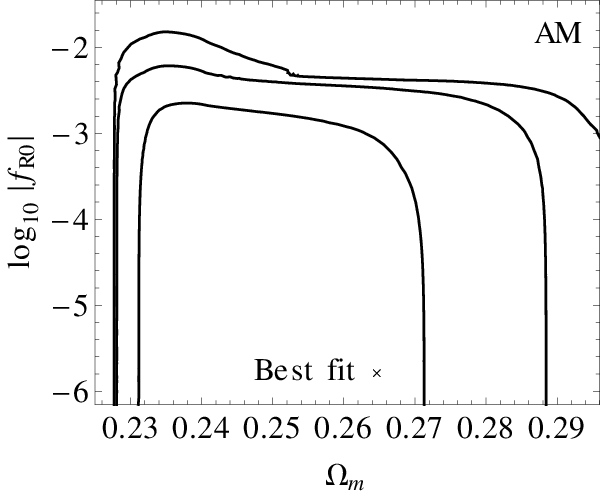
Fig. 4 shows that the $f(R)$ predictions in the AM case for $|f_{R0}|=10^{-3}$ are in clear tension with the data, at least when excluding scatter. Further, due to the strong radial dependence, the $f(R)$ effects cannot easily be canceled by varying some of the other cosmological parameters. This leads to a 1D-marginalized constraint of $|f_{R0}|<3.5\times 10^{-3}$ at the 95% confidence level. Note that including a prior on scatter plays an essential role (see Fig. 6), i.e., if we were to remove it from the analysis, very large scatter would make large $|f_{R0}|$ models viable (see Fig. 3 and Fig. 4) and due to a slow increase of the enhancement $A$ as function of $|f_{R0}|$ (see Fig. 2), there would be a rather loose constraint on $|f_{R0}|$. This is what happens if one wishes to constrain the TM scenario instead. In contrast to the AM case, when fixing the mass range equally in the $\Lambda$CDM and modified gravity model and therefore lowering the average halo mass within the stacked profiles, the discrepancy in the enhancement on $\Delta\Sigma$ on scales below $r_{\perp}\lesssim 1h^{-1}~\text{Mpc}$ and above $r_{\perp}\gtrsim 10h^{-1}~\text{Mpc}$ is less severe (see Fig. 1 and Fig. 4). Therefore, in that case, smaller values of scatter are already sufficient to make the profile enhancement compatible with the cluster-galaxy lensing data. This leaves $|f_{R0}|$ unconstrained within the region of applicability of our linearized $f(R)$ equations, $|f_{R0}|\lesssim 2\times 10^{-2}$. Note, however, that the TM case does not consistently take into account the enhanced abundance of clusters of $f(R)$ gravity and we, therefore, restrict our $f(R)$ specific constraints to the AM case.

Fig. 6 shows the 2D-marginalized likelihoods for the parameter degeneracies with $|f_{R0}|$ and Fig. 7 shows the one-tail 1D-marginalized likelihood for $|f_{R0}|$. In Fig. 8, we illustrate the band of $\xi_{\rm hm}$ and $\Delta\Sigma$ predictions bounded from below by the best-fit AM $f(R)$ gravity model, which is essentially identical to the best-fit concordance model ($|f_{R0}|=1.7\times 10^{-6}$), and from above by the upper 68% confidence level value of $|f_{R0}|$ with otherwise identical parameter values.

In the phenomenological case based on the TM halo profile enhancements, we use a Gaussian function in $\ln r$ with width and position fixed to fit the simulation and only consider the amplitude of the Gaussian function $F_{0}$ as an additional free parameter (see §IV.2). We obtain a mean and standard deviation of $F_{0}=0.34\pm 0.20$. Fig. 6 illustrates parameter correlations with $F_{0}$, Fig. 7 shows the two-tail 1D-marginalized likelihood for the amplitude $F_{0}$, and in Fig. 8 we present the best-fit predictions for $\xi_{\rm hm}$ and $\Delta\Sigma$. The best-fit parameter values, as well as the corresponding $-2\ln L$ are listed in Table 3.

$F_{0}=0$ corresponds to the $\Lambda$CDM model with DMO simulations and is consistent at the 1D-marginalized 95% confidence level (Fig. 7). The best fit is obtained for $F_{0}=0.34$, achieving $-2\Delta\ln L=-2.7$ with respect to the best-fit concordance model.

The data thus slightly prefer an enhancement in halo profiles over $\Lambda$CDM in the phenomenological case. Future surveys will thus either strengthen the constraints on modified gravity parameters, or even more interestingly, provide additional evidence for $F_{0}>0$. Note that for the best-fit $\Lambda$CDM model the reduced $\chi^{2}$ is roughly unity and that we therefore do not expect our error bars to be significantly underestimated.

The shape of the enhancement effect, $g(r)$, on the cluster profile $\xi_{\rm hm}$ and the excess surface mass density $\Delta\Sigma$ observed in $f(R)$ gravity simulations cannot be reproduced by any reasonable deviations in the parameter values of the fiducial cosmology (see Figs. 3 and 4). Our comparison of theoretical predictions to the lensing observable is, however, affected by the following possible scale-dependent systematics.

• •

  Mass scatter: In §III.3, we include a log-normal scatter in the mass-richness relation in our theoretical modeling. The actual form of the scatter might differ from log-normal, though it seems unlikely that this would result in an enhancement of $\Delta\Sigma$ localized at $r_{\perp}\simeq(1-10)h^{-1}~\text{Mpc}$.

• •

  Baryons: In order to understand the formation of galaxies within clusters, it is essential to include the baryonic components. Realistic models comprise mechanisms such as gas cooling, star formation, supernovae feedback, as well as the feedback from supermassive black holes to avoid the overcooling and accumulation of gas in the core of the cluster, the so-called active galactic nucleus (AGN) feedback. AGN outbursts produce shock waves that move the gas from the core to larger radii, i.e., between $r_{\rm v}$ and $2r_{\rm v}$, as was shown in [102] by employing simulations of Virgo-like galaxy clusters. Moreover, due to the AGN feedback, there is a slight adiabatic expansion of the dark matter when compared to DMO simulations (see Fig. 9 of [102]), leading to a $\lesssim 10\%$ effect on the density profiles. These effects have a radial dependence that is qualitatively different from the modified gravity enhancements considered here. Note that the moved mass by modified gravity can be calculated as

  $$\Delta M=4\pi\bar{\rho}\int_{0}^{\infty}\xi_{\text{hm}}(r)\mathcal{Q}(r)r^{2}dr$$

  (29)

  and amounts to $\Delta M\approx 6\times 10^{12}h^{-1}~M_{\odot}$ for the phenomenological fit with $F_{0}=0.3$.

• •

  Intrinsic alignment: High-precision weak-lensing measurements may be contaminated by the intrinsic alignment of galaxies (see, e.g., [103]). The correlation of intrinsic alignment and gravitational shear distortion can contribute to the observed ellipticity correlation function and $\Delta\Sigma$ at the $\lesssim 10\%$ level [104, 105].

• •

  Miscentering and satellites: The cluster centers in the MaxBCG sample are identified by the brightest cluster galaxy (BCG). The true cluster center may, however, be offset from the BCG position (see, e.g., discussion in [82]). This effect causes a suppression of the lensing signal in the inner parts of the halo, which subsequently leads to an underestimation of the cluster mass and the concentration. A miscentered $\Delta\Sigma$ can have a bump relative to a correctly centered $\Delta\Sigma$, which is, however, located further inwards than the $f(R)$ gravity enhancement (cf. [106]). A similar enhancement around the virial radius can further be introduced by galaxy satellites. To prevent the contamination of the excess surface mass density through satellites, we apply a cylindrical cut in the projected radius at $r_{\rm cut}=3r_{\rm v}$ in the simulations (see §III.2) and the observations (see §V). Note that we applied this cut only to the zhorizon simulations and not to the $f(R)$ gravity simulations. We verified, however, that changing $r_{\rm cut}$ has a negligible impact on the dependence of $\Delta\Sigma$ on cosmological parameters. Furthermore, the cut only affects $\Delta\Sigma$ on scales $r_{\perp}\gtrsim 5h^{-1}~\text{Mpc}$. Therefore, we can safely assume that there is no significant impact on the relative $f(R)$ enhancement by the cylindrical cut.

• •

  Wrong cosmology: The analysis of lensing as used in this study requires the assumption of an a priori cosmological model to estimate the critical surface mass density $\Sigma_{\text{crit}}$ and to convert angles to distances. Within $\Lambda$CDM, a wrong prior on the cosmological model produces a radial horizontal shift of $\Delta\Sigma$ at the $\lesssim 2\%$ level for $\Omega_{m}=0.25\pm 0.05$ (see discussion in [107]). Note that the Hu-Sawicki $f(R)$ gravity model matches the $\Lambda$CDM background to order $|f_{R0}|$. Deviations of this magnitude have a negligible impact on $\Delta\Sigma$.

• •

  Simulation systematics: In order to test the convergence of the halo profiles of the large-scale cosmological simulations on the scales used in this study, we compared the halo profiles from the zhorizon simulations to the halo profiles of the millennium simulations [108], which employ $N=2\,160^{3}$ particles in a $500^{3}h^{-3}~\text{Mpc}^{3}$ box. The profiles agree at the $\lesssim 5\%$ level on the scales of interest. We therefore conclude that the zhorizon simulations have converged for $r\sim(0.2-100)h^{-1}~\text{Mpc}$. The halos in the zhorizon simulations are identified using an FoF halo finder, while the $f(R)$ effects were measured on a SO-identified halo sample. However, since we only use the enhancements from the $f(R)$ simulations relative to $|f_{R0}|=0$, we expect the difference to be smaller than the residual statistical error ($\sim 20$%) on the modified gravity effects. Note that the environmental effects found in [97, 109] are induced by the chameleon mechanism and are not relevant for the values of $|f_{R0}|$ considered here. Moreover, halo finders typically agree at the scales relevant to our halo profile measurements [110].

• •

  Survey geometry: While we are mimicking the selection process as closely as possible, including the removal of fake clusters, the simulation measurements provide the dark matter and halo positions in a cubic box. Furthermore the simulation results are obtained from a single redshift slice at the effective redshift of the sample, and are thus not accounting for the redshift evolution of the lens sample.

References

- [1] C. M. Will, Living Rev. Rel. 9, 3 (2005), [arXiv:gr-qc/0510072].
- [2] W. Fang et al., Phys. Rev. D78, 103509 (2008), [arXiv:0808.2208].
- [3] L. Lombriser, W. Hu, W. Fang and U. Seljak, Phys. Rev. D80, 063536 (2009), [arXiv:0905.1112].
- [4] R. Reyes et al., Nature 464, 256 (2010), [arXiv:1003.2185].
- [5] Y.-S. Song, H. Peiris and W. Hu, Phys. Rev. D76, 063517 (2007), [arXiv:0706.2399].
- [6] T. Giannantonio, M. Martinelli, A. Silvestri and A. Melchiorri, JCAP 1004, 030 (2010), [arXiv:0909.2045].
- [7] L. Lombriser, A. Slosar, U. Seljak and W. Hu, arXiv:1003.3009.
- [8] A. Hojjati, L. Pogosian and G.-B. Zhao, JCAP 1108, 005 (2011), [arXiv:1106.4543].
- [9] F. Schmidt, A. Vikhlinin and W. Hu, Phys. Rev. D80, 083505 (2009), [arXiv:0908.2457].
- [10] C. Di Porto and L. Amendola, Phys. Rev. D77, 083508 (2008), [arXiv:0707.2686].
- [11] D. Rapetti, S. W. Allen, A. Mantz and H. Ebeling, Mon. Not. Roy. Astron. Soc. 400, 699 (2009), [arXiv:0812.2259].
- [12] S. F. Daniel et al., Phys.Rev. D80, 023532 (2009), [arXiv:0901.0919].
- [13] D. Rapetti, S. W. Allen, A. Mantz and H. Ebeling, Mon. Not. Roy. Astron. Soc. 406, 1796 (2010), [arXiv:0911.1787].
- [14] R. Bean and M. Tangmatitham, Phys.Rev. D81, 083534 (2010), [arXiv:1002.4197].
- [15] S. F. Daniel et al., Phys. Rev. D81, 123508 (2010), [arXiv:1002.1962].
- [16] S. F. Daniel and E. V. Linder, Phys. Rev. D82, 103523 (2010), [arXiv:1008.0397].
- [17] J. Dossett, M. Ishak, J. Moldenhauer, Y. Gong and A. Wang, JCAP 1004, 022 (2010), [arXiv:1004.3086].
- [18] I. Tereno, E. Semboloni and T. Schrabback, Astron. Astrophys. 530, A68 (2011), [arXiv:1012.5854].
- [19] G.-B. Zhao et al., Phys. Rev. D81, 103510 (2010), [arXiv:1003.0001].
- [20] J. Dossett, J. Moldenhauer and M. Ishak, Phys. Rev. D84, 023012 (2011), [arXiv:1103.1195].
- [21] J. N. Dossett, M. Ishak and J. Moldenhauer, Phys.Rev. D84, 123001 (2011), [arXiv:1109.4583].
- [22] L. Lombriser, Phys. Rev. D83, 063519 (2011), [arXiv:1101.0594].
- [23] G.-B. Zhao et al., arXiv:1109.1846.
- [24] T. L. Smith, arXiv:0907.4829.
- [25] R. Wojtak, S. H. Hansen and J. Hjorth, Nature 477, 567 (2011), [arXiv:1109.6571].
- [26] S. M. Carroll, V. Duvvuri, M. Trodden and M. S. Turner, Phys. Rev. D70, 043528 (2004), [arXiv:astro-ph/0306438].
- [27] S. Nojiri and S. D. Odintsov, Phys. Rev. D68, 123512 (2003), [arXiv:hep-th/0307288].
- [28] S. Capozziello, S. Carloni and A. Troisi, Recent Res. Dev. Astron. Astrophys. 1, 625 (2003), [arXiv:astro-ph/0303041].
- [29] A. A. Starobinsky, JETP Lett. 30, 682 (1979).
- [30] A. A. Starobinsky, Phys. Lett. B91, 99 (1980).
- [31] J. Khoury and A. Weltman, Phys. Rev. D69, 044026 (2004), [arXiv:astro-ph/0309411].
- [32] I. Navarro and K. Van Acoleyen, JCAP 0702, 022 (2007), [arXiv:gr-qc/0611127].
- [33] T. Faulkner, M. Tegmark, E. F. Bunn and Y. Mao, Phys. Rev. D76, 063505 (2007), [arXiv:astro-ph/0612569].
- [34] W. Hu and I. Sawicki, Phys. Rev. D76, 064004 (2007), [arXiv:0705.1158].
- [35] Y.-S. Song, W. Hu and I. Sawicki, Phys. Rev. D75, 044004 (2007), [arXiv:astro-ph/0610532].
- [36] F. Schmidt, M. Lima, H. Oyaizu and W. Hu, Phys. Rev. D79, 083518 (2009), [arXiv:0812.0545].
- [37] F. Schmidt, Phys. Rev. D80, 123003 (2009), [arXiv:0910.0235].
- [38] SDSS, B. Koester et al., Astrophys. J. 660, 239 (2007), [arXiv:astro-ph/0701265].
- [39] SDSS, K. N. Abazajian et al., Astrophys. J. Suppl. 182, 543 (2009), [arXiv:0812.0649].
- [40] L. Knox, Y.-S. Song and J. A. Tyson, Phys. Rev. D74, 023512 (2006).
- [41] F. Schmidt, Phys. Rev. D78, 043002 (2008), [arXiv:0805.4812].
- [42] B. Jain and P. Zhang, Phys. Rev. D78, 063503 (2008), [arXiv:0709.2375].
- [43] S. Tsujikawa and T. Tatekawa, Phys. Lett. B665, 325 (2008), [arXiv:0804.4343].
- [44] A. Borisov, B. Jain and P. Zhang, Phys.Rev. D85, 063518 (2012), [arXiv:1102.4839].
- [45] M. C. Martino, H. F. Stabenau and R. K. Sheth, Phys. Rev. D79, 084013 (2009), [arXiv:0812.0200].
- [46] F. Schmidt, Phys. Rev. D80, 043001 (2009), [arXiv:0905.0858].
- [47] T. Narikawa and K. Yamamoto, JCAP 1205, 016 (2012), [arXiv:1201.4037].
- [48] H. Oyaizu, Phys. Rev. D78, 123523 (2008), [arXiv:0807.2449].
- [49] H. Oyaizu, M. Lima and W. Hu, Phys. Rev. D78, 123524 (2008), [arXiv:0807.2462].
- [50] G.-B. Zhao, B. Li and K. Koyama, Phys. Rev. D83, 044007 (2011), [arXiv:1011.1257].
- [51] B. Li, G.-B. Zhao, R. Teyssier and K. Koyama, JCAP 1201, 051 (2012), [arXiv:1110.1379].
- [52] S. Ferraro, F. Schmidt and W. Hu, Phys. Rev. D83, 063503 (2011), [arXiv:1011.0992].
- [53] G. Squires and N. Kaiser, Astrophys. J. 473, 65 (1996), [arXiv:astro-ph/9512094].
- [54] R. E. Smith, Mon. Not. Roy. Astron. Soc. 400, 851 (2009), [arXiv:0810.1960].
- [55] A. Jenkins et al., Mon. Not. Roy. Astron. Soc. 321, 372 (2001), [arXiv:astro-ph/0005260].
- [56] WMAP, D. N. Spergel et al., Astrophys. J. Suppl. 148, 175 (2003), [arXiv:astro-ph/0302209].
- [57] WMAP, D. N. Spergel et al., Astrophys. J. Suppl. 170, 377 (2007), [arXiv:astro-ph/0603449].
- [58] R. E. Smith, C. Hernandez-Monteagudo and U. Seljak, Phys. Rev. D80, 063528 (2009), [arXiv:0905.2408].
- [59] V. Springel, Mon. Not. Roy. Astron. Soc. 364, 1105 (2005), [arXiv:astro-ph/0505010].
- [60] U. Seljak and M. Zaldarriaga, Astrophys. J. 469, 437 (1996), [arXiv:astro-ph/9603033].
- [61] R. Scoccimarro, Mon. Not. Roy. Astron. Soc. 299, 1097 (1998), [arXiv:astro-ph/9711187].
- [62] M. Crocce, S. Pueblas and R. Scoccimarro, Mon. Not. Roy. Astron. Soc. 373, 369 (2006), [arXiv:astro-ph/0606505].
- [63] M. Davis, G. Efstathiou, C. S. Frenk and S. D. M. White, Astrophys. J. 292, 371 (1985).
- [64] E. Rozo et al., Astrophys. J. 699, 768 (2009), [arXiv:0809.2794].
- [65] D. G. York et al., Astron. J. 120, 1579 (2000).
- [66] D. J. Eisenstein et al., Astron. J. 122, 2267 (2001).
- [67] G. T. Richards et al., Astron. J. 123, 2945 (2002).
- [68] M. A. Strauss et al., Astron. J. 124, 1810 (2002).
- [69] D. W. Hogg, D. P. Finkbeiner, D. J. Schlegel and J. E. Gunn, Astron. J. 122, 2129 (2001).
- [70] Ž. Ivezić et al., Astronomische Nachrichten 325, 583 (2004).
- [71] M. Fukugita et al., Astron. J. 111, 1748 (1996).
- [72] J. A. Smith et al., Astron. J. 123, 2121 (2002).
- [73] J. E. Gunn et al., Astron. J. 116, 3040 (1998).
- [74] R. H. Lupton et al., The SDSS Imaging Pipelines, in ASP Conf. Ser. 238: Astronomical Data Analysis Software and Systems X, pp. 269–+, 2001.
- [75] J. R. Pier et al., Astron. J. 125, 1559 (2003).
- [76] D. L. Tucker et al., Astronomische Nachrichten 327, 821 (2006), [arXiv:astro-ph/0608575].
- [77] K. N. Abazajian et al., Astrophys. J. Supp. 182, 543 (2009), [arXiv:0812.0649].
- [78] N. Padmanabhan et al., Astrophys. J. 674, 1217 (2008), [arXiv:astro-ph/0703454].
- [79] H. Aihara et al., Astrophys. J. Supp. 193, 29 (2011), [arXiv:1101.1559].
- [80] D. J. Eisenstein et al., Astron. J. 142, 72 (2011), [arXiv:1101.1529].
- [81] R. Mandelbaum, A. Tasitsiomi, U. Seljak, A. V. Kravtsov and R. H. Wechsler, Mon. Not. Roy. Astron. Soc. 362, 1451 (2005), [arXiv:astro-ph/0410711].
- [82] R. Mandelbaum, U. Seljak, T. Baldauf and R. E. Smith, Mon. Not. Roy. Astron. Soc. 405, 2078 (2010), [arXiv:0911.4972].
- [83] R. Reyes et al., arXiv:1110.4107.
- [84] C. Hirata and U. Seljak, Mon. Not. Roy. Astron. Soc. 343, 459 (2003).
- [85] R. Mandelbaum et al., Mon. Not. Roy. Astron. Soc. 361, 1287 (2005), [arXiv:astro-ph/0501201].
- [86] R. Feldmann et al., Mon. Not. Roy. Astron. Soc. 372, 565 (2006), [arXiv:astro-ph/0609044].
- [87] R. Nakajima et al., Mon. Not. Roy. Astron. Soc. 420, 3240 (2012), [arXiv:1107.1395].
- [88] G. M. Bernstein and M. Jarvis, Astron. J. 123, 583 (2002).
- [89] WMAP, J. Dunkley et al., Astrophys. J. Suppl. 180, 306 (2009), [arXiv:0803.0586].
- [90] C.-L. Kuo et al., Astrophys. J. 664, 687 (2007), [arXiv:astro-ph/0611198].
- [91] A. C. S. Readhead et al., Astrophys. J. 609, 498 (2004), [arXiv:astro-ph/0402359].
- [92] K. Grainge et al., Mon. Not. Roy. Astron. Soc. 341, L23 (2003), [arXiv:astro-ph/0212495].
- [93] Supernova Cosmology Project, M. Kowalski et al., Astrophys. J. 686, 749 (2008), [arXiv:0804.4142].
- [94] A. G. Riess et al., Astrophys. J. 699, 539 (2009), [arXiv:0905.0695].
- [95] B. A. Reid, L. Verde, R. Jimenez and O. Mena, JCAP 1001, 003 (2010), [arXiv:0910.0008].
- [96] W. J. Percival et al., Mon. Not. Roy. Astron. Soc. 401, 2148 (2010), [arXiv:0907.1660].
- [97] F. Schmidt, Phys. Rev. D81, 103002 (2010), [arXiv:1003.0409].
- [98] A. Lewis and S. Bridle, Phys. Rev. D66, 103511 (2002), [arXiv:astro-ph/0205436].
- [99] N. Metropolis, A. W. Rosenbluth, M. N. Rosenbluth, A. H. Teller and E. Teller, J. Chem. Phys. 21, 1087 (1953).
- [100] W. K. Hastings, Biometrika 57, 97 (1970).
- [101] A. Gelman and D. B. Rubin, Statist. Sci. 7, 457 (1992).
- [102] R. Teyssier, B. Moore, D. Martizzi, Y. Dubois and L. Mayer, Mon. Not. Roy. Astron. Soc. 414, 195 (2011), [arXiv:1003.4744].
- [103] J. Blazek, M. McQuinn and U. Seljak, JCAP 1105, 010 (2011), [arXiv:1101.4017].
- [104] C. M. Hirata et al., Mon. Not. Roy. Astron. Soc. 381, 1197 (2007), [arXiv:astro-ph/0701671].
- [105] J. Blazek, R. Mandelbaum, U. Seljak and R. Nakajima, arXiv:1204.2264.
- [106] S. Hilbert and S. D. M. White, Mon. Not. Roy. Astron. Soc. 404, 486 (2010), [arXiv:0907.4371].
- [107] T. Baldauf, R. E. Smith, U. Seljak and R. Mandelbaum, Phys. Rev. D81, 063531 (2010), [arXiv:0911.4973].
- [108] V. Springel et al., Nature 435, 629 (2005), [arXiv:astro-ph/0504097].
- [109] G.-B. Zhao, B. Li and K. Koyama, Physical Review Letters 107, 071303 (2011), [arXiv:1105.0922].
- [110] A. Knebe et al., Mon. Not. Roy. Astron. Soc. 415, 2293 (2011), [arXiv:1104.0949].
- [111] W. Hu and A. V. Kravtsov, Astrophys. J. 584, 702 (2003), [arXiv:astro-ph/0203169].
- [112] R. K. Sheth and G. Tormen, Mon. Not. Roy. Astron. Soc. 308, 119 (1999), [arXiv:astro-ph/9901122].
- [113] J. F. Navarro, C. S. Frenk and S. D. M. White, Astrophys. J. 490, 493 (1997), [arXiv:astro-ph/9611107].
- [114] J. S. Bullock et al., Mon. Not. Roy. Astron. Soc. 321, 559 (2001), [arXiv:astro-ph/9908159].
- [115] L. Lombriser, K. Koyama, G.-B. Zhao and B. Li, arXiv:1203.5125.