Semi-Parametric Drift and Diffusion Estimation for Multiscale Diffusions
Abstract
We consider the problem of statistical inference for the effective dynamics of multiscale diffusion processes with (at least) two widely separated characteristic time scales. More precisely, we seek to determine parameters in the effective equation describing the dynamics on the longer diffusive time scale, i.e. in a homogenization framework. We examine the case where both the drift and the diffusion coefficients in the effective dynamics are space-dependent and depend on multiple unknown parameters. It is known that classical estimators, such as Maximum Likelihood and Quadratic Variation of the Path Estimators, fail to obtain reasonable estimates for parameters in the effective dynamics when based on observations of the underlying multiscale diffusion. We propose a novel algorithm for estimating both the drift and diffusion coefficients in the effective dynamics based on a semi-parametric framework. We demonstrate by means of extensive numerical simulations of a number of selected examples that the algorithm performs well when applied to data from a multiscale diffusion. These examples also illustrate that the algorithm can be used effectively to obtain accurate and unbiased estimates.
Keywords. Parameter estimation, multiscale diffusions, stochastic
differential equations, homogenization, coarse-graining, effective dynamics
AMS subject classifications. 60H10, 60J60, 62M05, 34E13, 74Q99, 62F99
1 Introduction
Problems with multiple temporal and/or spatial scales emerge naturally in a wide variety of fields in science and engineering. From biological phenomena [8] and atmosphere and ocean science [40] to molecular dynamics [21], material science [15], fluid and solid mechanics [24, 26]. Many of such systems are often subject to noise that is either due to thermal fluctuations [13], randomness in the environment (e.g. uncertainty in some parameters) [25, 53, 51], coarse-graining of high-dimensional deterministic systems with random initial conditions [42, 57], or stochastic parameterization of small scale effects [12].
Mathematically the influence of noise in a system can be described by a single or coupled, nonlinear stochastic differential equations (SDEs) with multiple scales. In many cases these equations are high-dimensional but from a practical point of view only the evolution of some components of the solution is of main interest, since they act on a slower scale. It is therefore desirable to approximate the full system by an adequate simplified low-dimensional effective model (coarse-graining) that retains the essential dynamic characteristics of the full system. The effective equation is often amenable to analytical and numerical work. However, usually only the complete multiscale (fast/slow) system is directly observable but not the effective dynamics. Consequently, much research has been undertaken to find accurate approximations to the effective dynamics [19].
In many applications a wealth of data (i.e. observations of the fast/slow system) is often available and it is therefore worthwhile to use these data to determine the effective dynamics. However, extracting the effective dynamics directly from the available data is often not straightforward and it is thus important to adapt techniques from analysis, statistics, and numerical analysis to obtain appropriate coarse-grained models.
This data-driven coarse graining methodology has been applied to relatively simple (stochastic) systems for which a low dimensional coarse-grained equation exists, using techniques such as homogenization and averaging. For example, in [47] Brownian motion in a two-scale potential was studied. Therein, through both rigorous mathematical analysis and numerical simulations, it was shown that the estimation of drift and diffusion coefficients in the coarse-grained model is asymptotically biased when using classical estimators. Furthermore, it was shown that subsampling the available data at an appropriate rate between the two characteristic time scales of the full system is necessary for an accurate estimation of both drift and diffusion coefficients in the coarse-grained model. More general fast/slow systems of SDEs for which a coarse-grained equation exists were studied in [46] where it was shown that the same issue of asymptotically biased estimators persists in the homogenization framework – that is, when considering an effective dynamics on the (longer) diffusive time scale – and that appropriately subsampled data reduce the bias. These techniques were then applied to the problem of estimating eddy diffusivities from noisy Lagrangian observations in [9] where an improved algorithm that combines subsampling with appropriate averaging and variance reduction techniques was proposed and tested. Furthermore, inverse problems for multiscale partial differential equations – a problem closely related to that of parameter estimation – were studied in [45].
Although appropriate subsampling can potentially improve the
accuracy of estimators in the context of multiscale diffusions, as it
yields unbiased estimators, the
question of an optimal subsampling rate (i.e. the rate for which
the biased is removed) remains open; e.g. the studies in
[47, 46] provide only existence
results. Furthermore, the numerical experiments presented in the
aforementioned works indicate that the optimal subsampling rate is
not only problem dependent, but is also different for different
parameters in the same model. Consequently, an optimal subsampling
rate is in general unknown. The problem of identifying an optimal
subsampling rate for Gaussian processes has been studied in
[3, 4]; see also
[56] for related work in the context of econometrics.
Related problems have been studied in the context of numerical analysis for SDEs with multiple time scales. In particular, the heterogeneous multiscale method (HMM) [55, 12] is based on the idea of evolving the solution of the low-dimensional coarse-grained equation, when the coefficients in the coarse-grained equation are being evaluated “on the fly” by running short runs of the underlying fast dynamics. Similar ideas have been proposed in the framework of the “equation-free methodology” introduced by Kevrekidis and collaborators; see e.g. [54, 31, 30, 32]. Recently, the HMM methodology has been extended to approximate stochastic partial differential equations with multiple timescales [1]. As such, these techniques can be considered as a hybrid between numerical analysis and statistical inference since the coefficients in the coarse grained SDE are estimated from data that are obtained from short runs of the full dynamics. We emphasize, however, that in the HMM the fast dynamics is assumed to be known, whereas in the aforementioned works on parameter estimation for multiscale diffusions, as well as in the present work no such assumption is made.
We also mention that the effect of the multiscale structure on the evolution of the coarse-grained probability density using the Fokker-Planck equation (Kolmogorov’s forward equation) was studied in [17]. In this study it was shown that when decreasing the spatial discretization in a finite difference approximation the error increases rapidly and that in order to avoid this, it is necessary to improve the accuracy of the estimators of the drift and diffusion coefficients.
In many cases of interest the noise in the coarse-grained equation appears in a multiplicative way. One is thus confronted with the problem of estimating parameters in both the drift and the diffusion coefficients of an SDE of the form
with unknown parameters , the set of all feasible parameters. The problem is further complicated by the fact that the parameters and may not be independent as for example in the problem of Brownian motion in a two-scale potential, see Section 3.2.2. In the absence of multiscale effects in the data, or if one assumes that the optimal subsampling rate is known, a combination of the maximum likelihood estimator (MLE) and the quadratic variation of the path (QVP) is the most commonly used estimator in practice; see [52, 36, 37] for background material on classical estimators. The QVP (or a variant thereof) is used to estimate parameters in the diffusion coefficient and, based on these estimates, the MLE is used to obtain estimates for the parameters in the drift. As the MLE is based on an SDE with unit diffusion, one usually transforms the original SDE into an SDE with unit diffusion coefficient by applying Itô’s formula to
| (1) |
for an arbitrary in the state space of the process and replacing with the estimator obtained from the QVP for concreteness. For example, when considering
which is the diffusion coefficient in the coarse-grained equation of the stochastic Burgers’ equation (see Section 3.2.5), then transformation (1) reads
where has to be replaced by a previously obtained estimator.
Notice that this transformation can be singular when implementing it in practice,
so that special care has to be taken when performing numerical simulations.
In particular within the MLE framework where a (nonlinear) objective function
needs to be maximized, this might cause problems. An
alternative approach to estimate parameters is based on the MLE for
the discretized approximation, e.g. obtained by the Euler-Maruyama
scheme [33, ch. ], of the time-continuous SDE.
However, the non-vanishing (fixed) time-step size introduces an
additional bias so that even for simple models this approach does
not necessarily yield consistent estimators [38].
The main aim of the present study is to develop statistical inference techniques that enable us to estimate parameters in both drift and diffusion coefficients of a coarse-grained equation in the presence of an underlying (either stochastic or deterministic) multiscale structure in the fast/slow system. More precisely, given only observations of the slow component of the fast/slow system without any further knowledge of the fast component, the aim is to infer the coefficients in the coarse-grained equation. Furthermore, we wish to extend this approach in a semi-parametric framework, to situations where the drift and diffusion coefficients can be expanded in an appropriate (e.g. Taylor series) expansion.
Besides the lack of reliable statistical inference techniques for these problems, the motivation for this study originates also from recent results on the derivation of coarse-grained equations (also known as amplitude equations) for stochastic partial differential equations (SPDEs) with quadratic nonlinearities [6]. A typical example for such an SPDE is the stochastic Burgers’ equation
| (2) |
on equipped with appropriate boundary conditions. Therein denotes the covariance operator, space-time white noise, and . To study solutions to (2) of on time scales of , i.e. ensuring that we are in the regime described by amplitude equations, a diffusive rescaling is performed by defining via . Then solves
| (3) |
If the SPDE is equipped with homogeneous Dirichlet boundary conditions it can be shown that the dominant mode of the solution to (3) can be approximated by the solution to an one-dimensional SDE driven by classical Brownian motion of the form
Since this class of SPDEs arises in many different applications – from population biology [25] to fluid dynamics [51, 50] where many data are available – it is of major interest to obtain effective dynamics for the dominant modes of solutions to the SPDE by means of a data-driven coarse graining methodology.
The statistical inference technique we propose here consists of two
steps. First, we use the martingale property of the stochastic
integral to obtain an equation involving only the drift but not the
diffusion coefficient of the SDE. Since the drift might depend
on multiple (unknown) parameters, it is generally impossible to
obtain the parameters uniquely from a single equation. The
main element we employ to overcome this under-determined situation
is the often disregarded initial condition. In fact, by varying the
initial condition of the SDE one can define the estimator for the
drift parameters via the best approximation of a system of
equations. For the second step, we rely on the estimators for the
drift parameters and on the Itô isometry to obtain a relation
for the unknown parameters in the diffusion. Using the same idea as
in the first step, that is by varying the initial condition of the
SDE, we can also define the estimators for parameters concerning the
diffusion via the best approximation of a system of equations.
The expectations involved in both steps of
the estimation procedure are approximated by an average over many
short trajectories (i.e. by ensemble averages) in contrast to
classical estimators that often rely on a long trajectory
of the underlying process, see e.g. [52].
That is, the methodology we propose here relies on independent short
trajectories starting from different initial conditions.
The main practical advantages of the methodology proposed here can be summarized as follows:
- (a)
Coarse-grained models of high-dimensional, possibly infinite-dimensional, problems that retain the essential dynamic characteristic of the full system are a powerful tool to study problems arising in science and engineering. The simplicity of such an effective model, typically an SDE, makes it attractive for mathematical and numerical scrutiny. When the coefficients of the SDE can be computed exactly, the effective SDE allows us to decipher rapidly some of the basic characteristics of the full system, e.g. by computing first-passage properties and properties alike as it was done for instance in [51, 50]. However, in several problems it is not straightforward to obtain the coefficients of the coarse-grained SDE exactly due to the complexity of the underlying full system. From a theoretical standpoint several assumptions need to be made, e.g. the dynamics is dominated by a single eigenfunction/mode (often associated with a symmetry in the system) and the higher-order modes decay sufficiently fast (see the derivation of the “phase-diffusion” equation describing the transverse instability of propagating waves/fronts; e.g. in [35, 28]), to obtain computable coefficients. Conversely, from a practical point of view obtaining approximations (estimators) of the coefficients in the coarse-grained model, which can be used to study the basic characteristics of the full system, is very appealing.
- (b)
A model for a physical or technological process might not be readily available, either because its derivation is cumbersome, or it is not straightforward to formulate it from first principles. But the underlying physics of the phenomena at hand and previous experience with similar systems suggests an SDE of the form adopted here, at least in certain regions of the parameter space. In a spirit similar to the equation-free approach, one can utilize available data and obtain a low-dimensional approximation to the process, which in turn can be used as a model for the process in regions of the parameter space consistent with the assumptions imposed from the outset. But often such models can be applicable in regions beyond those dictated by the assumptions. For instance, for a long-wave instability such as that observed on a surface of a film flowing down an inclined plane [29] the growth rate curve of infinitesimal disturbances extends from the origin up to a cut-off wavenumber. The Landau-Stuart equation is then only applicable sufficiently close to the cut-off, i.e. it can be used to describe the transition when an unstable wave motion of given (“fundamental”) wavenumber interacts with its first stable harmonics. On the other hand, when the growth rate curve has a “nose” near criticality consistent with a short-wave instability and so that the system equilibrates to a stationary norm solution in the nonlinear regime, such as with with Rayleigh-Bénard convection [10], the Landau-Stuart equation can be applicable even past the instability threshold.
The rest of the paper is organized as follows. In Section 2 we present the precise derivation of the estimators for systems with and without multiscale structure. Based on these results, in Section 3 the general applicability and performance of the prosed methodology is investigated via different numerical examples. The extensive numerical study we undertake illustrates that the proposed technique enables us to estimate accurately parameters in multiscale diffusions. A summary of the results and future perspectives are offered in Section 4.
2 Estimators
We present the precise derivation of the drift and diffusion estimators for systems without and systems with multiscale effects present. First we outline the methodology for SDEs without multiscale structure and illustrate some properties of the estimators in this case, before presenting the set-up for multiscale diffusions.
2.1 Derivation of Drift and Diffusion Estimators
For the sake of simplicity we consider here only one dimensional real-valued processes (see Sections 3.2.3 and 3.2.4 for examples of multivariate processes). Consider the scalar-valued Itô stochastic differential equation
| (4) |
where denotes standard one-dimensional Brownian motion. Both the drift coefficient and the diffusion coefficient are assumed to be sufficiently smooth such that the SDE provides a unique solution for any initial condition and on any finite time interval; see e.g. [34, sec. ]. Moreover, we assume that both drift and diffusion depend on unknown parameters and the task is to estimate the parameters in and from available data. In fact, here we focus on the case when and are polynomials in of degree and , respectively, where denote index sets of finite cardinality and respectively. The unknown coefficients of the polynomials are and respectively, i.e. we consider
| (5) |
Consequently, and are linear functions in and , respectively. These particular assumptions on the drift and the diffusion simplify the notation in what follows and they will lead to a linear system of equations for the estimators of the parameters. Notice that parameterization (5) is not compulsory and also other parameterizations, such as for some known functions , will lead to linear system of equations for . More general parameterizations will, however, not necessarily result in a system of linear equations for anymore and more elaborated methods (e.g. an iterative approach using Newton’s method) are required.
The starting point in the derivation of the estimators is based on the following identities
| (6a) | ||||
| (6b) | ||||
owing to the martingale property of the stochastic integral and the
Itô isometry, respectively, holding for any fixed initial
condition . The next step is to incorporate the
parameterization of the functions and into
(6), to identify the functional structure of the
relation for the parameters and , respectively.
We begin with substituting the parameterization of into equation
(6a), which will yield an estimator for the
parameter , that is present in the drift term alone.
Based on this estimator it is possible to proceed similarly with
equation (6b) and
eventually obtain an estimator for the parameter present in the diffusion part.
Substituting ansatz (5) for into (6a) yields
| (7) |
for a given initial condition . Therein denotes the expectation with respect to the Wiener measure and with respect to processes starting at a fixed initial condition . To emphasize this dependency on the initial condition we will use the notation . Fix a time (the question how to chose the final time will be addressed in Section 3) and define
With these definitions equation (6a) can be rewritten as
| (8) |
The above equation is under-determined for . To derive a well-defined estimator for , we consider a finite sequence of initial conditions with . Since (8) is valid for each initial condition, this approach yields a system of linear equations
| (9) |
with and . The linear system does not have a unique solution in general (if a solution exists at all). To overcome this shortcoming we define the solution of the system of linear equations in (9), i.e. the estimator of the drift parameter, to be the best approximation
respectively,
| (10) |
with being the Moore-Penrose pseudo-inverse [5]. We note that the estimation of parameters in the drift does not require knowledge of the diffusion coefficient.
Assume now that we have already estimated the parameters in the drift correctly. Then substituting the ansatz (5) of into (6b) yields
Recall again that the expectation is with respect to the Wiener measure and processes starting at , hence . To cope with multiple parameters, we follow the same approach as for the drift parameters above. In fact, define here
and consider again a finite sequence of initial conditions . Then we also obtain a system of linear equations for the parameters
| (11) |
with and . We define the estimator again via the best approximation
| (12) |
Since the estimation of diffusion parameters is based on the estimators for the drift parameters, additional error sources might affect the estimator in practice – see Section 2.3 for an example of this error propagation.
In practice we are confronted with discrete observations instead of continuous ones, so that we need to approximate the (deterministic) integrals in , , and . Assume that we have observations at equidistant times for and . The goal is to approximate the integrals by means of these observations. Since the integrands depend on the path of the solution of an SDE, we cannot expect the integrands to be very smooth. For such “rough” functions the trapezoidal rule is more accurate than Simpson’s rule [11]. Consequently, we approximate the various integrals via the composite trapezoidal rule
| (13) |
where we used that and .
2.2 Description of the Algorithm: An Example
To apply the actual parametric estimation procedure introduced in the previous section to a specific problem, not only data need to be available but also a parameterization needs to be chosen. Consequently, the complete algorithm can be understood as consisting of two stages:
- 1.
Initialization: The time step is given by the underlying time series of observations and is assumed to be constant (however, this assumption is not necessary, in fact, the procedure might be carried out in the exact same manner with a non-equidistant sampling rate) and the terminal time is fixed by choosing appropriately (cf. Section 3). Expectations are approximated by averages over trajectories generated form independent Brownian motions. The crucial step is to fix a parameterization for both drift and diffusion coefficients. Lastly, the sequence of initial conditions needs to be chosen appropriately.
- 2.
Two-step Estimation: Based on the initializations in the previous stage the estimators are well-defined. According to Section 2.1 the parameters and are estimated successively, first the parameters in the drift and then the parameters in diffusion coefficient. For both estimators, two steps need to be performed:
- (a)
- (b)
Since the estimation step depends on the considered parameterizations for drift and diffusion, we present a detailed pseudocode of the methodology in Algorithm 1
for the example using and , i.e. with
| (14) |
This setting corresponds to the Landau-Stuart equation that will play a vital role in the numerical examples discussed in Section 3. The input arguments of Algorithm 1 are the time step size and the data array . The dimension of the array is a result of different initial conditions each with trajectories of observations. When we denote by the value at time of the -th trajectory started initially in , then corresponds to the collection of these trajectories at discrete (equidistant) times. For the example we consider here, we define approximations of the first three moments at time via
Thus, the quantities defining the matrices and right-hand sides involved in the estimation step (cf. (9) and (11), respectively) are approximated via
| (15a) | ||||
| (15b) | ||||
with and denoting the quadrature operator of the trapezoidal rule on with equally spaced () subintervals (cf. (13))
| (16) |
It should be emphasized that equations such as (e.g. as in lines and in Algorithm 1) are merely meant as a formal notation for solving the least squares problem , , cf. equations (10) and (12), rather than indicating that we first compute and then multiply it with to obtain , a step which clearly is computationally inefficient. In practice the method to compute the solution typically depends on the rank of . For the numerical examples that we will present in Section 3 we ensured a full rank situation by considering a sufficiently large number of different initial conditions. The solution can be computed with one of the several methodologies for solving least squares problems, e.g. the Cholesky factorization of the normal equations11 1 This method for solving the least squares problem is simple to implement but might not be optimal and is usually only recommended for problems with large residuals. However, it is noteworthy that for the numerical examples presented in this study, the method performed well and no stability issues occurred (as can be demonstrated by monitoring the condition number; not shown here), and similar results were obtained with a QR factorization with column pivoting (not shown here). ; for details on such methodologies we refer to standard textbooks on numerical linear algebra, e.g. [20, ch. ].
2.3 Properties of the Estimator
The proposed estimation procedure relies on two key ingredients. The first is that the methodology is based on the identities in (6). The second is that by considering a finite sequence of initial conditions we can cope with multiple parameters in drift and diffusion coefficient, respectively. In the sequel we demonstrate the influence of both components on the proposed estimation scheme with the help of some elementary, nonetheless illustrative, examples when no multiscale effects are present. A detailed and rigorous analysis of the proposed methodology for both multiscale and non-multiscale situations will be presented elsewhere.
To illustrate the influence on the identities in (6) and to address some asymptotic properties we consider a simple Langevin equation with additive noise
The drift estimator proposed in this study – this parameterization is already a straightforward generalization of the one introduced above – relies on the relation
| (17) |
with being the true value. For a fixed final time , the estimator for continuous-time observations – meaning that we approximate only the expectation by an average but do not approximate the integrals – based on a single (fixed) initial condition is given by
| (18) |
Notice that we dropped the dependency on the initial condition, because only a single initial condition is considered here. Since we approximate only the expectations by finite averages, it is not surprising that the estimator for continuous-time observations (18) converges to the true value in agreement with the law of large numbers. The property that the variance of the error vanishes for reflects the fact that the estimator relies on an identity, i.e. on a direct (deterministic) computation (17) rather than on asymptotic time limits (i.e. on ergodicity).
Recall that we have observations at times with fixed, in the case of discrete-time observations. The integral approximation introduces an additional error that can be identified via
| (19) |
with an appropriate constant that depends not only on but also on and , and which vanishes in the limit as . Here denotes the quadrature operator of the trapezoidal rule as defined in (16). The actual error of the trapezoidal rule depends on the regularity of the integrand. Here we rely only on the assumption as a general scenario and do not discuss the rate of convergence. Then, similarly to the continuous-time case, the estimator (when neglecting sampling errors) can be written as
| (20) |
with being the average error constant. Hence, the integral approximation introduces an additional bias – second term in the bracket – that can be controlled by . Notice that so that the additional bias vanishes as for every . Consequently, from equation (20) one infers that for a fixed final time , one should choose both to obtain an accurate estimate.
To estimate the diffusion coefficient the proposed scheme relies on the relation
that is valid for all times and where we replace by its estimator for concreteness. Consequently, the estimator for continuous-time observation using a single (fixed) initial condition and a fixed final time reads
Since the estimator for the diffusion coefficient depends on the estimated drift parameter, an additional error is introduced (last two terms), as expected. To illustrate the asymptotic properties of the estimator we, however, assume that the error is negligible. Consequently, we find that
where denotes the Chi-squared distribution with degrees of freedom. Recall that for sufficiently large, as a consequence of the central limit theorem.
For the modification of discrete-time observations the integrals are again approximated via the trapezoidal rule. Based on the same observations (neglecting sampling errors) at and fixed we find
with being the error representation of the trapezoidal rule, cf. (19). In contrast to the continuous-time situation, the term reflects the additional error due to the integral approximation that can be controlled by . Since this additional term is the only difference, expanding the square yields a similar result as in the continuous-time situation. If we assume again that the error from the drift parameter is negligible, then we find
| (21) |
with . Since for every , the second term in equation (21) can only be controlled by . Consequently, for a fixed final time , choosing is necessary to obtain an accurate estimate of the true parameter. It is noteworthy that the same steps may be carried out for an arbitrary diffusion function, but obviously we cannot directly infer the distributions of terms involving the stochastic integral.
To deal with multiple parameters in drift and/or diffusion coefficients the proposed estimation scheme relies on considering a finite sequence of initial conditions and defining the estimator via the best approximation. To illustrate the effect of this second component of the estimation procedure, consider the SDE
Provided all quantities are well defined, the estimator of , via a best approximation using a sequence of initial conditions , is given by
where and are as in (8) associated with the drift function . On the other hand, the quantity yields a local estimator for each initial condition because the considered problem has only one parameter to be determined. Thus the best approximation corresponds here to the weighted arithmetic mean of these local estimators with weights . Consequently, increasing includes an additional stabilization effect into the estimation scheme. From this point of view, the best approximation resolves naturally the problem of combining local estimates to a global estimator that arises in different estimation procedures as well, where piecewise local strategies are utilized to improve the estimates; see for example [7]. In this study a heuristic estimation strategy for non-constant diffusions in the MLE framework is proposed by extracting local information from a large time-series to estimate coefficients locally and combine these local estimators to global estimators. Since this strategy is based on the MLE, the results in the above study also highlight the subsampling issue when applied to multiscale diffusions.
It should be noted that although the proposed methodology computes moments of the solution of an SDE, there is no direct link to the generalized method of moments (GMM) [23]. The GMM for parametric estimation for SDEs is more closely related to the MLE instead, as both estimation schemes rely on ergodicity of the corresponding process by using long time-series. In fact, both estimators even coincide for many cases [22, ch. ]. Since the MLE is biased for multiscale diffusions, it can be expected that the subsampling issue also arises for the GMM when applied to data obtained form a system with multiscale structure.
2.4 Estimators for Multiscale Diffusions
In the context of diffusion processes with two widely separated time scales we consider the following set-up: A fast/slow system of SDEs
| (22a) | ||||
| (22b) | ||||
equipped with appropriate initial conditions. In (22) denote Brownian motions of appropriate dimensions and denotes a small parameter. For the dimension of the fast/slow system we assume that and (for simplicity) , where denotes a finite time interval of interest. Furthermore, we assume that drift and diffusion functions in (22a) and (22b) respectively, are such that there exists a well-defined (i.e. the SDE provides a unique weak solution on any finite time interval and for any initial condition) coarse-grained SDE
| (23) |
in the limit of ; see e.g. [48, ch. 11 and 18] and references therein for technical details. That is, the slow process is approximated by the solution of (23) for . Even in cases where both the effective drift and the effective diffusion function are known, the actual computation of these expressions might be difficult or even impossible, as appropriate Poisson equations have to be solved and integrals with respect to the invariant measure of the fast process to be computed. Hence, our goal is to estimate both effective drift coefficient and effective diffusion coefficient in (23) from available data (observations) of the fast/slow system (22) (more precisely, only of its slow component). To this end we assume the same parameterizations of the effective drift and diffusion functions as introduced in Section 2.1:
where we recall that denote index sets with and . Our goal then is: Given observations only of the slow component (22a), is it possible to estimate the parameters and characterizing the associated coarse-grained equation (23)? Under the assumption that the (ergodic) fast process (22b) is stationary, the algorithm described in Section 2.1 applies straightforwardly also for this problem, given the final time of observation length is appropriately chosen; cf. Section 3.2. That is, using multiple initial conditions for the slow process (22a) to deal with multiple parameters in drift and diffusion, while the fast process is sampled from its invariant measure that is assumed to be known, either analytically or numerically.
The main motivation to consider the same algorithm also in the presence of multiscale effects originates from the fact that both the slow component of the full fast/slow system and the effective dynamics have probability laws that are approximately the same, provided . Consequently, also expectations with respect to these laws are approximately equal. Since the proposed methodology is based on expectations, cf. equation (6), we believe that this approach yields asymptotically unbiased estimators. A rigorous analysis of the proposed methodology to verify this heuristic argument is currently work in progress and will be reported elsewhere.
We conclude this section with a remark on a recently proposed estimator for constant diffusion coefficients [16] that can also be derived using the approach we introduce here. To this end, assume that the coarse-grained equation takes the form:
where we assume that the effective drift is known and we wish to estimate the diffusion coefficient from available data of a fast/slow system. When considering a single (fixed) initial condition and following the approach introduced in Section 2.1, the resulting estimator reads
where the integrals are being approximated by a quadrature rule and is chosen appropriately (in fact, we have approximated the Lebesgue integral via the trapezoidal rule). If one, however, uses a rectangular-method with the left corner node instead, this estimator coincides with the estimator proposed in [16] for estimating the effective diffusion coefficient based on observations of the slow component of a fast/slow system. We emphasize, that a crucial assumption on the estimator in the aforementioned work is that the effective drift is known a priori. This assumption is very restrictive and makes the estimator unfeasible for most practical applications. A further limitation of the estimator in [16] is that it applies only in situations where the noise in the coarse-grained equation is additive (constant diffusion coefficient). Conversely, the methodology proposed here aims to estimate multiple parameters in both the drift and the diffusion coefficients.
3 Numerical Experiments
We now present numerical experiments of parameter estimations for diffusion processes to illustrate the behavior of the estimation scheme developed in Section 2.
3.1 Parameter Estimation for single-scale SDEs
Let us first present numerical results for parameter estimation when no multiscale effects are present. We investigate two different SDEs. In Section 3.1.1 we consider the SDE corresponding to the Ornstein-Uhlenbeck process and in Section 3.1.2 we examine the stochastic Landau-Stuart equation. The purpose of these examples is twofold. On the one hand they are used to illustrate that the proposed methodology can be employed successfully in practice to estimate unknown parameters and on the other they help us understand the influence of the parameters , , , and on the algorithmic estimation procedure. The time series were obtained by solving the corresponding SDEs via the Euler-Maruyama scheme. In all numerical examples reported in this section, we used a time step of .
3.1.1 Ornstein-Uhlenbeck Process
Consider the following SDE
| (24) |
with the unique solution being the Ornstein-Uhlenbeck process starting at . The estimation procedure is applied to data from the SDE with true parameters using a variety of different values for the parameters of the algorithm.


Figure 1 depicts the relative errors of the estimated values as functions of the number of initial conditions for different combinations of (recall that the final time is ) and . For the estimated drift parameter (Figure 1(a)) there is a discrepancy among different combinations of and for small values of and the relative errors vary from approximately to . Increasing decreases the relative errors, with fluctuations due to the discretization, as expected; cf. Section 2.3. Moreover, it is apparent that the larger and , the smaller the relative error. In contrast to the drift parameter, the relative errors of the diffusion parameter (Figure 1(b)) are already small (relative error smaller than ) even for small values of . This is due to the constant diffusion coefficient of the SDE. Increasing generally decreases the relative error further, again, with fluctuations due to the discretization. We note that although an error propagates from the drift estimation to the diffusion estimation (cf. Section 2), it appears to be negligible in this example. Based on theses results, it seems plausible to tune the algorithm-defining parameters in a way such that the estimators provide a given relative accuracy while at the same time the computational cost is minimized. Obviously the question of optimized algorithm-defining parameters is of high importance in practical applications. However, this is not a straightforward issue to address as not only the discretization related parameters and influence the accuracy of the algorithm in practice, but also the number of initial conditions as well as their locations; we will investigate these and related issues in a future study, see also the discussion in Section 4.
3.1.2 Landau-Stuart Equation
Consider the stochastic Landau-Stuart equation [35, ch. ], where both additive and multiplicative noise are present
| (25) |
This SDE can be obtained from a wide class of spatially extended systems, e.g. the noisy Kuramoto-Sivashinsky equation [51, 50] by assuming near-critical conditions, i.e. being sufficiently close to the primary bifurcation, and employing the homogenization theory developed in [6]. In this case we need to estimate a total number of four parameters, two in the drift and two in the diffusion coefficient.


We performed various numerical experiments with different choices of parameters. Figure 2 illustrates the relative error of the estimated parameters as functions of the number of initial conditions for different combinations of and when the true parameters are . We find qualitatively the same behavior as in the previous section for the Ornstein-Uhlenbeck process: all three parameters , , and affect the accuracy of the estimators. Although the Figures 2(a)–2(d) show a decreasing trend of the relative errors when increasing , fluctuations are still present. These fluctuations are of different magnitude for different parameters and are reduced by increasing both and . One also observes that increasing improves the accuracy of the estimators but only up to a certain level, i.e. the corresponding curves approach nearly constant values for large , that are due to the approximation of the original system matrix, for instance in (9), by a matrix based on observations and the aforementioned discretizations. Although it is apparent that estimating all parameters in the Landau-Stuart model is more delicate than for the Ornstein-Uhlenbeck process in Section 3.1.1, it nonetheless seems possible to determine optimal algorithm-defining parameters such that the computational cost is minimized given a certain error tolerance for the estimators for this model also.
3.2 Parameter Estimation for Fast-Slow Systems
Of particular interest is the behavior of the estimator when applied to systems with two different time scales. We examine the properties of the estimation scheme for stochastic multiscale diffusions (Sections 3.2.1–3.2.3), the problem of estimating the eddy diffusivity in a two-dimensional cellular flow (the Taylor-Green flow, Section 3.2.4), truncated systems of time rescaled stochastic partial differential equations (Section 3.2.5), and deterministic systems that exhibit temporal chaos that can be approximated by an appropriate SDE (Section 3.2.6). To measure the accuracy of the estimation procedure in these examples, we rigorously derive the coarse-grained equations from the associated fast/slow systems using homogenization theory so that the theoretical coefficients are known. Based only on observations of the slow component of the fast/slow system, the goal is to infer the coefficients in the coarse-grained equation using the proposed estimation procedure. The estimated values are then compared with the theoretical ones. It is noteworthy that no assumptions on the knowledge of the fast component, nor on the structure of the fast/slow system are made (also is unknown). As the precise dependency of the estimation procedure on the control parameters is still an open question, the main purpose of this section is to illustrate the general applicability of the proposed estimation procedure for multiscale diffusions. If not stated otherwise, the generated time series were obtained by solving the corresponding multiscale SDEs via the Euler-Maruyama scheme using a time step . Furthermore, the expectation is approximated by an average using independent Brownian paths and different (equally-spaced) initial conditions are used. We emphasize once again that this particular choice of algorithm-defining parameters might be far from optimal in the sense of computational complexity. But since our main goal is to demonstrate the applicability of the proposed scheme to multiscale diffusions, these algorithm-defining parameters will yield reliable estimators.
3.2.1 Fast Ornstein-Uhlenbeck Noise
When the fast process is an Ornstein-Uhlenbeck process it is rather straightforward to determine the precise form of the effective equation associated to the fast/slow system, because this task reduces to computing Gaussian integrals. Consider for example
| (26a) | ||||
| (26b) | ||||
with being a standard Brownian motion, then the effective dynamics is given by
| (27) |
where denotes the average of with respect to the invariant measure of the fast process (Ornstein-Uhlenbeck process). We note that we have subtracted the Stratonovich correction from the drift in (26a), so that the noise in (27) can be interpreted in the Itô sense.22 2 The noise entering (26a), i.e. the process (26b), is a smoothed approximation to white noise, so that the noise in the limiting equation has to be interpreted in the Stratonovich sense according to the Wong-Zakai theorem. Correcting the drift is not essential for the applicability of our methodology, it was done so that the limiting equation (27) is somewhat simpler. In the sequel we consider two different choices of the pair . As a first example let
| (28) |
then the amplitude equation is precisely the Ornstein-Uhlenbeck process (cf. Section 3.1.1) but here in the context of multiscale diffusions where classical estimators fail. To illustrate this failure and motivate the necessity of an appropriate sampling rate, the quadratic variation of the path (QVP) estimator for the effective diffusion constant and the maximum likelihood estimator (MLE) for the effective drift parameter are applied to a time series on with initial condition generated by the associated fast/slow system (26) with true parameters and .


Figure 3(a) depicts the performance of both the QVP and the MLE as functions of the subsampling rate . The parameter indicates here that only every -th observation is used to estimate the parameters in the drift and diffusion coefficients, hence denotes the time period between two consecutive observations. Starting from the case without subsampling (, that is ) and increasing , both estimators approach the true value. However, after an optimal subsampling rate, for which the estimator is as close to the true value as possible (here approximately , that is ), both estimators deviate monotonically from the target value. We note that at the optimal subsampling rate the relative error is approximately . Figure 3(a) seems to suggest that the optimal subsampling rate is given by the local extremum of the estimator as function of the subsampling. However, this behavior is not true in general, see for instance the numerical examples in [47, 16] that reveal different behaviors. Recall, that the optimal subsampling rate is in general unknown.
The situation is different when the effective parameters are
estimated via the method introduced here. Observations are
generated by the associated fast/slow system
(26) with true parameters and . The performance of the estimator
as function of the final time for both and
is plotted in Figure 3(b) and is
compared directly to the results obtained by the classical
estimators discussed before. For small values of one observes
that the estimated value of the drift parameter fluctuates
around the true value and stabilizes for larger times with minor
fluctuations around the true value. We note that the estimator
obtained by the proposed scheme significantly outperforms the MLE in
terms of accuracy.33
3
At the optimal subsampling rate the relative error for the MLE is
approximately 10%, whereas the relative error for the drift parameter obtained by the novel scheme is
less than 1% for . Admittedly, this comparison is not completely fair, because
the novel estimation scheme in its current form relies on more data than the MLE, but we believe that
these numbers nonetheless illustrate the potential of the methodology we propose.
For the estimated diffusion coefficient
one finds that the novel scheme proposed here and the
QVP estimator yield similar results for small values of ,
indicating that increasing here has the same beneficial
effect as subsampling does for the QVP estimator. But unlike the
QVP, the estimator proposed here approaches the correct value
further and closely fluctuates around it when increasing ,
without any deviations as when using QVP and subsampling. This is a
typical behavior for the estimator when applied to multiscale
diffusions as we will see in the forthcoming examples.
Consequently, one finds that, unlike classical estimators, once the
final time is larger than a critical value, the estimator
fluctuates closely around the true value.
Consider as a second example and , so that the fast/slow system (26) reads
| (29a) | ||||
| (29b) | ||||
with the effective dynamics in (27) given by the Landau Stuart equation (see Section 3.1.2)
| (30) |
A natural extension of the QVP estimator to diffusion coefficients that depend on multiple parameters is obtained by considering the standard QVP relation for different time increments. Provided that one considers a sufficient number of increments, i.e. a sufficient number of estimating equations, one can define the QVP estimator by solving the arising system. To illustrate that this approach can deal with multiple parameters in the diffusion coefficient when no multiscale effects are present in the data, we first use the QVP to estimate and in (30) based on data that are also obtained from (30). This (single-scale) situation corresponds to the classical case of parametric estimation and the QVP can indeed be used to obtain accurate estimators and , as it is illustrated in table 11(a).
Therein the obtained estimators and are presented for different values of , where indicates the number of independent Brownian paths that have been used to compute an average to improve the accuracy. The Landau-Stuart equation (30) was solved numerically on starting at with true parameters . Apparently, the QVP yields very accurate estimates in this setting. However, things change when the QVP is adopted in the presence of multiple time scales. In this multiscale setting we wish to estimate the parameters and in the effective dynamics (30) from observations of the slow component (29a) of the fast/slow system (29). The same true parameters and configuration (i.e. same number and length of time increments) of the QVP as in the classical example without multiscale effects were used, since the QVP performed well therein. Table 11(b) displays the obtained estimators and for different values of when the observations are obtained from (29) with scale separation . Increasing yields QVP estimators with minor fluctuations but both estimators are strongly biased, as expected. Hence, an appropriate subsampling of the data would be required to remove the bias, but, once again the optimal subsampling rate is not known a priori and might, as in the case of the MLE, even be different for different parameters.
Conversely, we will use

this example to illustrate that the parameters in multiscale diffusions can be estimated accurately using the proposed scheme, even though the amplitude equation provides a far more involved structure than the one of the previous example in addition to the multiscale structure of the problem. Figure 4 depicts the performance of the estimation procedure based on observations generated by the fast/slow system (29) with true parameters and as a function of the final time . The true values are indicated by dashed lines. The behavior of the estimators is qualitatively similar with that in the previous example. By increasing , the estimators approach the true values, respectively and fluctuate closely around them after a critical final time. Consequently, all parameters can be estimated accurately.
3.2.2 Brownian motion in a two-scale potential: A quadratic potential in one dimension
Here we study the example that was originally used in [47] to illustrate the failure of classical estimation schemes in the context of multiscale diffusions for the first time. More precisely we consider the first-order Langevin equation
| (31) |
which is a simple model to describe the movement of a Brownian particle in a two-scale potential subject to thermal noise – being a standard Brownian motion. Here we consider the one-dimensional problem (a two-dimensional example is treated in see Section 3.2.2) and further assume that the two-scale potential is given by a large scale as well as a fluctuating part: . Based on these assumptions we can rewrite the Langevin equation as
When the fluctuating part is sufficiently smooth and periodic with period , the effective dynamics is given by
| (32) |
where the effective coefficients are given by and , where , see [47] for details. Here we consider and , so that (32) is the SDE of an Ornstein-Uhlenbeck process with
where denotes the modified Bessel function of first kind, cf. [2, ch. ]. We note that both the effective drift and the effective diffusion depend on the diffusion of the original fast/slow system44 4 We remark that in the numerical examples presented in [16, sec. ] the drift coefficient in the homogenized equation is assumed to be known when estimating the diffusion coefficient, even though it depends explicitly on the unknown .. Figure 5 shows the performance of the estimation scheme when applied to observations of the fast/slow system with and .

As for the examples in the previous section both estimators and are biased for small final times . Using longer time series, i.e. increasing , reduces this bias and both estimators approach the true values (dashed lines) respectively.
3.2.3 Brownian motion in a two-scale potential: A quadratic potential in two dimensions
As a first example to illustrate that the proposed methodology can readily be extended to multivariate processes, we consider here a generalization of (31) in two dimensions
where denotes again a two-scale potential with being a set of parameters controlling the drift and denotes a standard two-dimensional Brownian motion. As with the one-dimensional case, we assume that the two-scale potential is given by a large scale as well as a fluctuating part, with the fluctuating part being separable: , with and . Hence, the original system reads
with . We take the large scale part to be a quadratic potential
with being symmetric and positive definite, so that the effective dynamics is given by
| (33) |
for with analytic expressions for ; see [47]. With and we find
where denotes again the modified Bessel function of the first kind.
Since both identities in (6) have pendants for multivariate processes, the methodology introduced here can be readily applied to estimate both effective drift matrix and the effective diffusion matrix in (33). The only difference is that the system of equations corresponding to (9) and (11), respectively, is a matrix equation in this case, and similar techniques to obtain the best approximation (both formally and numerically) can be employed [49]. Figure 6


depicts the performance of the estimation scheme when applied to observations of the fast/slow system with , , and . Figure 6(a) shows the estimated values of the four effective drift coefficients: As for the one-dimensional examples, the estimators also show here an approaching behavior towards the target values when increasing , yielding an accurate estimate of for sufficiently large. The same behavior when increasing is also observed for the estimated (diagonal) effective diffusion coefficient , as it is shown in Figure 6(b). We note that although the curves in Figure 6(b) show a minor gap for larger , the relative error is less than in both cases for .
3.2.4 Eddy diffusivity for the Taylor-Green flow
Here we use our estimator to estimate the eddy diffusivity (effective diffusion coefficient) of a tracer particle moving in a two-dimensional cellular flow and subject to molecular diffusion. This is a very well studied problem and it is known that the position of the tracer particle converges, under the diffusive rescaling, to a Brownian motion with a diffusion coefficient (covariance matrix) that can be calculated in terms of the solution of an appropriate Poisson equation, see e.g. [41] or [48, ch. ]. The equation for the position of the tracer particle is
where is a periodic divergence-free velocity field and denotes the small-scale diffusivity. In the numerical simulations below we will take to be the Taylor-Green flow, where and . We set to obtain the equation
| (34) |
In the limit as tends to , converges weakly to a Brownian motion with diffusion tensor , the eddy diffusivity. The goal here is to obtain an estimator of using the proposed methodology. It is known that the off-diagonal elements of the eddy diffusivity for the Taylor-Green flow vanish, and that the two diagonal elements are equal, and our numerical experiments are consistent with these results. Figure 7 shows the performance of diagonal elements of using (34) with and .


Even though is not known explicitly as a function of , it can be approximated accurately either by solving the Poisson equation using a spectral method or by performing a long time Monte Carlo simulation [9]. In the aforementioned work the value has been reported as an approximation of the diagonal elements. When a time step is used, Figure 7(a) shows that the estimators behave qualitatively in the same way as in the previous examples: increasing drives the estimators towards limiting values. Noteworthy is that although there are differences between these limiting values of the estimators and the target value (dashed horizontal line), the relative error is less than in both cases for . Moreover, the differences in 7(a) are mainly due to temporal discretizations and not due to multiscale effects as can be verified with Figure 7(b) where the performance of the estimators for the same experiment but with a smaller time step is shown.
3.2.5 Truncated Burgers’ Equation
We consider here an appropriately rescaled variant of the stochastic Burgers’ equation
on equipped with homogeneous Dirichlet boundary conditions. Under technical assumptions on the covariance operator of the space-time white noise , one can show (see [1] and references therein for details) that the coefficients of the three-term truncated representation of the solution have to solve the following multiscale SDE
with and being independent standard Brownian motions. Therein the covariance operator is such that noise acts only on the fast modes directly. For the truncated system standard homogenization theory applies and yields
| (35) |
as the effective dynamics with true parameters
See [6] for details. Figure 8 shows the performance of the estimation scheme when applied to observations of the three dimensional fast/slow system with , , and .

Since the true values of the effective coefficients (dashed lines) are of different orders for these particular choices, a semi-logarithmic scale is adopted for the sake of clarity. The plots show qualitatively the same behavior as in the previous examples when increasing the final time and suggest that the estimation procedure yields accurate estimators. Only the estimated value fluctuates around the true value. We note that the true value is very small () so that this coefficient has only marginal influence in the complete diffusion function. Furthermore, recall that even the time-step in the Euler-Maruyama discretization is larger (), so that the fluctuations are expected to be due to discretization errors. As a matter of fact, considering a finer discretization (i.e. increasing , and ) reduces the fluctuations (not shown here).
3.2.6 Fast chaotic noise
Our methodology is also applicable to a system of ordinary differential equations (ODEs) where the stochastic noise is replaced by deterministic chaos. In particular, we will consider an ODE driven by one of the components of an appropriately rescaled Lorentz system. More precisely, consider as an example the following system
| (36a) | ||||
| (36b) | ||||
| (36c) | ||||
| (36d) | ||||
where the fast component solves the Lorenz equation. In the sequel we investigate two different couplings between the fast and the slow process by choosing .
According to [48, ch. ] (see also [19, ex. ]), when eliminating the fast chaotic variable , the approximate dynamics for is given by
| (37) |
with and the diffusion coefficient that is given by the Green-Kubo formula
| (38) |
Therein with denoting the solution of the fast process at time when and . The convergence of the solution of (36a) to the solution of (37) can be justified rigorously using the recent results from [43]. However, the above expression for is not useful practically: Not only does it not give an analytical value for , also using it to obtain numerically is computationally expensive. Hence, it would be advantageous to use the methodology proposed here and estimate the effective coefficients via observations of the complete (deterministic) fast/slow system. To illustrate numerically that our estimation procedure can indeed deal with this problem, we apply it to observations of the deterministic fast/slow system using and to estimate both the drift and the diffusion coefficients. Since the system is deterministic, classical solvers for ODEs may be employed. For example, depending on the stiffness (i.e. on ) of the system, either a fourth order Runge-Kutta scheme or a solver based on numerical differentiation formulas is used.


Figure 9 depicts the estimated values as functions of the final time for two different choices of the scale separation . The value is the same with that used in [19], thus allowing for direct comparisons to be made; we will return to this point shortly. The estimated drift parameter (Figure 9(a)) shows (for both values of ) the typical behavior we expect in the context of multiscale diffusions. While the estimator is biased for small values of , increasing significantly reduces the bias so that the estimator approaches the true value (dashed line). The estimators of the effective diffusion coefficient (Figure 9(b)) also approach a limiting value when increasing , with minor fluctuations for both values of . In both plots, one observes a performance difference of the estimators for different values of . In fact, the more distinctive the scale separation (i.e. the smaller ) between fast and slow components, the faster the estimators approach a limiting value.
For both drift and diffusion estimator the curves for different values of give slightly different values
at time . Hence for there exists an additional bias, which is the reason for the observed difference in the estimators for different . On the other hand, one expects that as decreases the estimators of the effective coefficients become more accurate, as one observes here for the estimated drift . Thus, is also expected to be more accurate as decreases. Since no analytic formula for the diffusion coefficient exists, the estimator is compared with alternative numerical approximations available in [19, ex. and ill. ]. In the numerical experiments performed in this study the value was adopted giving a value of using Gaussian (second) moment approximations based on a modified Euler-Maruyama discretization of the effective dynamics, and a value of based on the heterogeneous multiscale method (HMM) with a discretization of the Green-Kubo formula for the effective diffusion coefficient; see also [14] for more elaborated HMM based numerical schemes applied to the Lorenz 96 model. Thus, we have a very good agreement of the result obtained by the estimation proposed here with these previously reported values. It is worth to mention that, unlike the procedure introduced here, the methods employed to determine the effective diffusion coefficient in [19] assume that the effective drift parameter is known. While the HMM can easily be adapted to the case of an unknown drift parameter, it is not straightforward to incorporate the unknown drift parameter in the estimation based on Gaussian moment approximations. In any event, incorporating the drift estimation would yield an even larger statistical error for these methods, while the results based on the presented scheme show only minor fluctuations; see Figure 9.
Choosing in (36a) and following the methodology outlined in [48, ch. ], yields the following effective dynamics
| (39) |
The effective coefficients are now given by
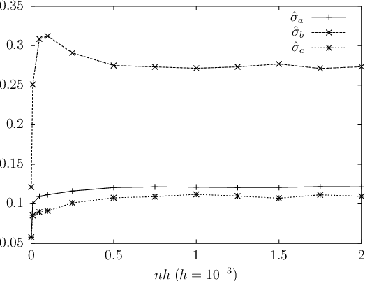
with being as in (38). We apply our methodology again to observations of the deterministic fast/slow system using , , and to estimate all six effective coefficients. Figure 10 illustrates the estimated values of both drift and diffusion parameters as functions of the final time .

4 Conclusion
We have developed a numerical methodology for estimating multiple parameters in a coarse-grained equation (in one or multiple dimensions) based on observation from an associated fast/slow system that posses a multiscale structure. This problem is far from straightforward, not only due to the multiscale effects present in the available data, but also due to difficulties associated with estimating parameters when both the drift and the diffusion coefficients are state dependent.
The approach developed in this study combines a number of different techniques. On the one hand, the derivation of the estimators relies on simple identities based on the martingale property for stochastic integrals and Itô isometry. On the other, we exploit our freedom in varying the initial condition in combination with standard techniques from inverse problems to define the parameter estimators via best approximation.
We demonstrated via a detailed numerical study that the proposed inference scheme provides us with accurate estimates for parameters in both the drift and the diffusion coefficients in systems with multiscale structure and state dependent noise. In fact, the proposed methodology appears to be accurate and effective even when the stochastic noise in the system is replaced by deterministic chaos.
While the feasibility study of the parameter estimation for multiscale diffusions and the initial presentation of the estimation scheme is the main development here, clearly many open problems and questions remain to be addressed. One such open question is the rigorous analysis of the algorithm to investigate its asymptotic properties and to scrutinize its limitations. Furthermore, the rigorous analysis of the algorithm is expected to reveal insights into the dependency on the algorithm-defining parameters that in turn can be used to reduce the computational complexity of the methodology.
Clearly, from a practical point of view there are different strategies to improve the efficiency of the estimators. A first starting-point could be the usage of techniques with an accelerated convergence instead of the brute-force Monte Carlo sampling to approximate the involved expectations, e.g. quasi Monte Carlo [44] or variance reduction techniques [33, ch. ]. Also recent work on Multilevel Monte Carlo methods [18] appears very appealing in this context, although care might have to be taken due to the nonlinear nature of the underlying model SDE; cf. [27].
Several questions also arise naturally within the presented framework of varying the initial condition to set up a system of equations: How many initial conditions need to be considered? Where to locate the initial conditions: Equispaced or distributed differently? How does the choice of the initial condition influence the accuracy of the estimator? In fact, preliminary numerical experiments suggest that an alternative distribution of the initial conditions improves the accuracy. Hence, an “optimal” distribution of the initial condition is expected to reduce the computational cost considerably.
Another interesting point concerns the best approximation. Here, we defined the estimator as the element that minimizes the residual of a linear system of equations with respect to the Euclidean norm. Thus, natural questions are, e.g. as to whether an alternative norm might be more appropriate, and how regularizing the minimization problem (e.g. by a truncated singular value decomposition or a Tikhonov regularization) affects the estimator. Also methodologies that “optimize” the linear system of equations to obtain more accurate best approximations, as they are for instance used in the reconstruction of tomographic problems [39], are appealing.
From a computational point of view, employing parallel computing strategies seem also promising. In fact, the presented algorithm consists of multiple parts (mainly when generating the observations) without mutual dependency. Thus, these parts lead to problems that are straightforward to parallelize.
There are applications, however, where only one long time-series is available, rather than several short ones, as required for the methodology developed here to estimate the drift and diffusion coefficients. It is an interesting question whether this methodology can be extended to cases where a long time-series is available only. This and related issues will be treated in feature studies.
Acknowledgements
We are grateful to the anonymous referees for insightful comments and suggestions. We also thank R. Nürnberg and A. M. Stuart for critically reading an earlier version of the manuscript and for their useful comments and suggestions. This work is supported by the Engineering and Physical Sciences Research Council of the UK through Grant No. EP/H034587.
References
- [1] A. Abdulle and G. A. Pavliotis, Numerical Methods for Stochastic Partial Differential Equations with Multiple Scales, J. Comput. Phys., 231 (2012), pp. 2482–2497.
- [2] M. Abramowitz and I. A. Stegun, Handbook of Mathematical Functions with Formulas, Graphs and Mathematical Tables, Dove, New York, 1964.
- [3] R. Azencott, A. Beri, and I. Timofeyev, Adaptive Sub-sampling for Parametric Estimation of Gaussian Diffusions, J. Stat. Phys., 139 (2010), pp. 1066–1089.
- [4] , Parametric Estimation of Stationary Stochastic Processes under Indirect Observability, J. Stat. Phys., 144 (2011), pp. 150–170.
- [5] A. Ben-Israel and T. N. E. Greville, Generalized Inverses: Theory and Applications, CMS Books in Mathematics, Springer, 2003.
- [6] D. Blömker, M. Hairer, and G. A. Pavliotis, Multiscale Analysis for Stochastic Partial Differential Equations with Quadratic Nonlinearities, Nonlinearity, 20 (2007), pp. 1721–1744.
- [7] C. P. Calderon, Fitting Effective Diffusion Models to Data Associated with a "Glassy" Potential: Estimation, Classical Inference Procedures, and Some Heuristics, Multiscale Model. Simul., 6 (2007), pp. 656–687.
- [8] A. Chauvière, L. Preziosi, and C. Verdier, eds., Cell Mechanics: From Single Scale-Based Models to Multiscale Modeling, Mathematical & Computational Biology Series, Chapman & Hall/CRC, 2010.
- [9] C. J. Cotter and G. A. Pavliotis, Estimating eddy diffusivities from noisy Lagrangian observations, Commun. Math. Sci., 7 (2009), pp. 805–838.
- [10] M. C. Cross and P. C. Hohenberg, Pattern formation outside of equilibrium, Rev. Modern Phys., 65 (1993), pp. 851–1112.
- [11] D. Cruz-Uribe and C. J. Neugebauer, Sharp Error Bounds for the Trapezoidal Rule and Simpson’s Rule, JIPAM. J. Inequal. Pure Appl. Math., 3 (2002), pp. 1–22.
- [12] W. E, D. Liu, and E. Vanden-Eijnden, Analysis of multiscale methods for stochastic differential equations, Comm. Pure Appl. Math., 58 (2005), pp. 1544–1585.
- [13] A. Einstein, Investigations on the Theory of Brownian Movement, Dover Publications, 1956. edited with notes by R. Fürth, translated by A. D. Cowper.
- [14] I. Fatkullin and E. Vanden-Eijnden, A computational strategy for multiscale systems with applications to lorenz 96 model, J. Comput. Phys., 200 (2004), pp. 605–638.
- [15] J. Fish, Multiscale Methods: Bridging the Scales in Science and Engineering, Oxford University Press, 2009.
- [16] Y. Frederix and D. Roose, Drift-Filtered Approach to Diffusion Estimation for Multiscale Processes, in Coping with Complexity: Model Reduction and Data Analysis, A. N. Gorban and D. Roose, eds., vol. 75 of Lecture Notes in Computational Science and Engineering, Springer, 2011, pp. 269–286.
- [17] Y. Frederix, G. Samaey, and D. Roose, An analysis of noise propagation in the multiscale simulation of coarse Fokker-Planck equations, ESAIM Math. Model. Numer. Anal., 45 (2011), pp. 541–561.
- [18] M. B. Giles, Multilevel Monte Carlo path simulation, Oper. Res., 56 (2008), pp. 607–617.
- [19] D. Givon, R. Kupferman, and A. M. Stuart, Extracting macroscopic dynamics: model problems and algorithms, Nonlinearity, 17 (2004), pp. 55–127.
- [20] G. H. Golub and C. F. van Loan, Matrix Computations, Johns Hopkins Studies in the Mathematical Sciences, Johns Hopkins University Press, 3rd ed., 1996.
- [21] M. Griebel, S. Knapek, and G. W. Zumbusch, Numerical Simulation in Molecular Dynamics: Numerics, Algorithms, Parallelization, Applications, Texts in Computational Science and Engineering, Springer, 2007.
- [22] J. D. Hamilton, Time Series Analysis, Princeton University Press, 1994.
- [23] L. P. Hansen, Large Sample Properties of Generalized Method of Moments Estimators, Econometrica, 50 (1982), pp. 1029–1054.
- [24] M. F. Horstemeyer, Multiscale Modeling: A Review, in Practical Aspects of Computational Chemistry, J. Leszczynski and M. K. Shukla, eds., Springer, 2010, pp. 87–135.
- [25] W. Horsthemke and R. Lefever, Noise-Induced Transitions: Theory and Applications in Physics, Chemistry, and Biology, vol. 15 of Springer Series in Synergetics, Springer, 1984.
- [26] P. Huerre and M.Rossi, Hydrodynamic instabilities in open flows, in Hydrodynamic and Nonlinear Instabilities, C. Godrèche and P. Manneville, eds., Cambridge University Press, 1998, pp. 81–294.
- [27] M. Hutzenthaler, A. Jentzen, and P. E. Kloeden, Divergence of the multilevel Monte Carlo Euler method for nonlinear stochastic differential equations. To appear in Ann. Appl. Probab. (2013).
- [28] S. Kalliadasis, Nonlinear instability of a contact line driven by gravity, J. Fluid Mech., 413 (2000), pp. 355–378.
- [29] S. Kalliadasis, C. Ruyer-Quil, B. Scheid, and M. G. Velarde, Falling Liquid Films, vol. 176 of Applied Mathematical Sciences, Springer, 2012.
- [30] I. G. Kevrekidis, C. W. Gear, and G. Hummer, Equation-free: The computer-aided analysis of complex multiscale systems, AIChE J., 50 (2004), pp. 1346–1355.
- [31] I. G. Kevrekidis, C. W. Gear, J. M. Hyman, P. G. Kevrekidis, O. Runborg, and C. Theodoropoulos, Equation-Free, Coarse-Grained Multiscale Computation: Enabling Microscopic Simulators to Perform System-Level Analysis, Commun. Math. Sci., 1 (2003), pp. 715–762.
- [32] I. G. Kevrekidis and G. Samaey, Equation-Free Multiscale Computation: Algorithms and Applications, Annu. Rev. Phys. Chem., 60 (2009), pp. 321–344.
- [33] P. E. Kloeden and E. Platen, Numerical Solution of Stochastic Differential Equations, Springer, 1992.
- [34] N. V. Krylov, On Kolmogorov’s equations for finite dimensional diffusions, in Stochastic PDE’s and Kolmogorov equations in infinite dimensions (Cetraro, 1998), vol. 1715 of Lecture Notes in Mathematics, Springer, 1999, pp. 1–63.
- [35] Y. Kuramoto, Chemical Oscillations, Waves, and Turbulence, Chemistry Series, Dover Publications, 2003. Slightly corrected republication of the work originally published by Springer in 1984.
- [36] Y. A. Kutoyants, Statistical Inference for Ergodic Diffusion Processes, Springer, 2004.
- [37] R. S. Liptser and A. N. Shiryaev, Statistics of Random Processes: I. General Theory, Stochastic Modelling and Applied Probability Series, Springer, 2nd ed., 2010. Translated by A. B. Aries.
- [38] A. W. Lo, Maximum Likelihood Estimation of Generalized Itô Processes with Discretely Sampled Data, Econometric Theory, 4 (1988), pp. 231–247.
- [39] H. Lustfeld, J. A. Hirschfeld, M. Reißel, and B. Steffen, Enhancement of precision and reduction of measuring points in tomographic reconstructions, Phys. Lett. A, 375 (2011), pp. 1167–1171.
- [40] A. J. Majda, C. Franzke, and B. Khouider, An applied mathematics perspective on stochastic modelling for climate, Philos. Trans. R. Soc. Lond. Ser. A Math. Phys. Eng. Sci., 366 (2008), pp. 2427–2453.
- [41] A. J. Majda and P. R. Kramer, Simplified models for turbulent diffusion: theory, numerical modelling, and physical phenomena, Phys. Rep., 314 (1999), pp. 237–574.
- [42] R. M. Mazo, Brownian Motion: Fluctuations, Dynamics, and Applications, International Series of Monographs on Physics, Oxford University Press, 2002.
- [43] I. Melbourne and A.M.Stuart, A Note on Diffusion Limits of Chaotic Skew Product Flows, Nonlinearity, 24 (2011), pp. 1361–1367.
- [44] H. Niederreiter, Random Number Generation and Quasi-Monte Carlo Methods, CBMS-NSF regional conference series in applied mathematics, Society for Industrial and Applied Mathematics, 1992.
- [45] J. Nolen, G. A. Pavliotis, and A. M. Stuart, Multiscale Modelling and Inverse Problems, in Numerical Analysis of Multiscale Problems, O. L. I.G. Graham, T.Y. Hou and R. Scheichl, eds., vol. 83, Springer, 2012, pp. 1–34.
- [46] A. Papavasiliou, G. A. Pavliotis, and A. M. Stuart, Maximum likelihood drift estimation for multiscale diffusions, Stochastic Process. Appl., 119 (2009), pp. 3173–3210.
- [47] G. A. Pavliotis and A. M. Stuart, Parameter Estimation for Multiscale Diffusions, J. Stat. Phys., 127 (2007), pp. 741–781.
- [48] , Multiscale Methods: Averaging and Homogenization, Springer, 2008.
- [49] R. Penrose, On best approximate solutions of linear matrix equations, Math. Proc. Cambridge Philos. Soc., 52 (1956), pp. 17–19.
- [50] M. Pradas, G. A. Pavliotis, S. Kalliadasis, D. T. Papageorgiou, and D. Tseluiko, Additive noise effects in active nonlinear spatially extended systems, European J. Appl. Math., 23 (2012), pp. 563–591.
- [51] M. Pradas, D. Tseluiko, S. Kalliadasis, D. T. Papageorgiou, and G. A. Pavliotis, Noise Induced State Transitions, Intermittency, and Universality in the Noisy Kuramoto-Sivashinksy Equation, Phys. Rev. Lett., 106 (2011), pp. 060602–1–060602–4.
- [52] B. L. S. Prakasa Rao, Statistical Inference for Diffusion Type Processes, vol. 8 of Kendall’s Library of Statistics, Arnold, 1999.
- [53] N. Savva, S. Kalliadasis, and G. A. Pavliotis, Two-Dimensional Droplet Spreading over Random Topographical Substrates, Phys. Rev. Lett., 104 (2010), pp. 084501–1–084501–4.
- [54] C. Theodoropoulos, Y.-H. Qian, and I. G. Kevrekidis, "Coarse" Stability and Bifurcation Analysis Using Time-Steppers: A Reaction-Diffusion Example, Proc. Natl. Acad. Sci. USA, 97 (2000), pp. 9840–9843.
- [55] E. Vanden-Eijnden, Numerical techniques for multi-scale dynamical systems with stochastic effects, Commun. Math. Sci., 1 (2003), pp. 385–391.
- [56] L. Zhang, P. A. Mykland, and Y. Aït-Sahalia, A Tale of Two Time Scales: Determining Integrated Volatility with Noisy High-Frequency Data, J. Amer. Statist. Assoc., 100 (2005), pp. 1394–1411.
- [57] R. Zwanzig, Nonequilibrium Statistical Mechanics, Oxford University Press, 2001.