Fréchet means of curves for signal averaging and application to ECG data analysis
Abstract
Signal averaging is the process that consists in computing a mean shape from a set of noisy signals. In the presence of geometric variability in time in the data, the usual Euclidean mean of the raw data yields a mean pattern that does not reflect the typical shape of the observed signals. In this setting, it is necessary to use alignment techniques for a precise synchronization of the signals, and then to average the aligned data to obtain a consistent mean shape. In this paper, we study the numerical performances of Fréchet means of curves which are extensions of the usual Euclidean mean to spaces endowed with non-Euclidean metrics. This yields a new algorithm for signal averaging without a reference template. We apply this approach to the estimation of a mean heart cycle from ECG records.
Keywords: Signal averaging; Mean shape; Fréchet means; Curve registration; Geometric variability; Deformable models; ECG data.
AMS classifications: Primary 62G08; secondary 62P10.
Acknowledgements - The author acknowledges the support of the French Agence Nationale de la Recherche (ANR) under reference ANR-JCJC-SIMI1 DEMOS.
1 Introduction
In many applications (biology, medicine, road traffic data) one observes a set of signals that have a similar shape. This may lead to the assumption that such observations are random elements which vary around the same but unknown mean shape. Signal averaging is then the process that consists in computing a mean curve which reflects the typical shape of the observed signals. This procedure generally amounts to find an appropriate combination of the data to compute an average shape with a better signal-to-noise ratio. In many situations, the observed signals exhibit not only a classical source of random variation in amplitude, but also a less standard geometric source of variability in time. Due to this source of geometric variability, the usual Euclidean mean of the raw data may yield a mean curve that does not reflect the typical shape of the signals, as illustrated by the following application.
1.1 Signal averaging in ECG data analysis
An important application of signal averaging is the estimation of a mean heart cycle from electrocardiogram (ECG) records. An ECG signal corresponds to the recording of the heart electrical activity. It is a signal, recorded over time, that is composed of the succession of cycles of contraction and release of the heart muscle. Each recorded cycle is a curve composed of a characteristic P-wave, reflecting the atrial depolarization, that is followed by the so-called QRS complex which corresponds to the depolarization of the ventricles, and which ends with a T-wave reflecting the repolarization of the heart (see e.g. [GH06] for a precise description of an ECG recording). In this paper, we present results on two different data sets from the MIT-BIH database [GAG+13]. In Figure 1(a), we display data from an ECG record of a healthy subject having no arrhythmia, and in Figure 1(b) we display data from an ECG record of a subject showing evidence of significant arrhythmia (note that, in all the figures showing ECG data, units on the vertical axis are in millivolts).
In the analysis of ECG data, it is generally assumed that the heart electrical activity repeats itself. Therefore, during an ECG record, one classically considers that the heart cycle of interest remains approximately the same with every beat, and that it is embedded in a random white noise with zero expectation that is uncorrelated with the mean shape to be estimated. After an appropriate segmentation of an ECG record, one observes a set of signals of the same length such that each of them contains a single QRS complex. The preliminary segmentation step is done by taking segments (of the same length) in the ECG record that are centered around the easily detectable maxima of the QRS complex of the beats. Identification of these maxima can be done using statistical methods to identity local extrema in noisy signals [Big06, GK95] or by applying appropriate digital filters to identify typical parts of the QRS complex [PT85]. In this paper, we used the approach in [Big06] to identify local maxima and to segment the ECG record into signals of the same length containing a single QRS complex. After this preliminary segmentation, one thus observes signals with approximately the same shape. In the normal case, we obtained signals displayed in Figure 2, while in the case of cardiac arrhythmia we obtained signals displayed in Figure 3.
To estimate the typical shape of a heart cycle and to improve the signal-to-noise ratio, one may use the Euclidean mean of these signals. In the normal case, this leads to satisfactory results as shown in Figure 4 since the average signal displayed in Figure 4(a) clearly reflects the typical shape of the heart beats displayed in Figure 4(b)-(g). However, in the case of cardiac arrhythmia, the electrical activity of the heart is more irregular. This can be seen in the shape of the heart beats displayed in Figure 3(b)-(g) which may vary significantly from one pulse to another. Due to noise and geometric variability in the measurements, a simple averaging step may cause a low-pass filtering effect that leads to a mean cycle that does not reflect the typical shape of the heart beats in the ECG record [RR86b, RR86a, LJB03]. In the case of cardiac arrhythmia, the Euclidean mean causes a low-pass filtering effect in the shape of the QRS complex, as shown by the results displayed in Figure 5. Indeed, it can be seen in Figure 3 that, around the time point (which corresponds to the beginning of the QRS complex) there is rapid transition between a flat region and the peak of the R wave. For the Euclidean mean displayed in Figure 5(a), this transition is slower, and it can be seen that the average heart cycle in Figure 5(a) is a convolution by a smooth kernel of the signals in Figure 3(b)-(g) around the time point . To obtain better results, it is necessary to use alignment techniques for a precise synchronization of the heart beats, and then to average the aligned data.


1.2 Deformable models
Assume for simplicity that the signals are observed on the time interval , and that they can be extended outside by periodicity. An alignment technique consists in finding a time synchronization of a set of signals. To be more precise, define a deformation operator parametrized by as a smooth increasing function such that
In the paper, we shall consider the following families of deformation operators:
- -
-
Translation operators: and , for () and all .
- -
-
Non-rigid operators: is diffeomorphism of parametrized by some , i.e. a smooth increasing function with and (a general method for constructing non-rigid deformation operators is described in Section 2.4).
Given and a family of deformation operators, the problem of time synchronization of two signals is to find a such for all . In ECG data analysis, the most widely used alignment technique is time synchronization using translation operators by temporal or multiscale cross-correlation, see [LJB03, TIR11] and references therein.
In the presence of variability in amplitude and shape in the data, it is reasonable to suppose that the signals at hand satisfy the following deformable (or perturbation) model:
| (1.1) |
where denotes the -th observation for the -th signal and are equi-spaced design points in . The function in model (1.1) is the unknown mean shape of the signals. The are supposed to be i.i.d. normal variables with zero expectation and variance . They represent a standard white noise in the measurements. The ’s are supposed to be independent of the ’s and are i.i.d. realizations of a smooth random process with zero expectation. Therefore, the ’s represent smooth variations in amplitude of the signals around . Finally, the ’s are assumed to be i.i.d. random variables in with zero expectation. Hence, the random deformation operators represent geometric variability in time in the data.
Note that the deformable model (1.1) is well adapted to ECG data processing. The main type of perturbations related to the analysis of ECG data (see e.g. [LJB03, TIR11]) are the baseline wandering effect (a low-frequency signal), electromyographic (EMG) noise, and power-line interference which is an amplitude and frequency varying sinusoid. This source of additive noise is modeled in (1.1) by the zero-mean processes . The physiological nature of the electrocardiographic signal also alters the recording from heartbeat to heartbeat in lag and duration. In the ECG signal, there are therefore variations in time of the heart cycle from one beat to another. This makes the heartbeats look shorter or longer in duration. After the segmentation of an ECG record into signals containing a single QRS complex, this local variability in time is modeled in (1.1) by the non-rigid deformation operators . Aligning heart beats using non-rigid deformation operators is an alternative to the cross-correlation method which is classical used in ECG data analysis. One of the goals of this paper is to show that using non-rigid operators to align signals obtained by the segmentation of an ECG record may significantly improve the shape of the mean heart cycle computed by averaging the data after a standard alignment using cross-validation.
1.3 Fréchet means of curves
The problem of estimating and the deformation parameters in model (1.1) has been studied in [BC11] using the following procedure. First, for each , smooth the data to construct an estimator of . In this paper, this smoothing step is done either by low-pass Fourier filtering or by wavelet thresholding. In a second step, estimate simultaneously the deformation parameters by minimizing the following criterion
| (1.2) |
where
| (1.3) |
and
Finally, in a third step take
| (1.4) |
as an estimator of the mean shape .
As explained in [BC11], the estimator can be interpreted as a smoothed Fréchet mean of the observed signals. The Fréchet mean [Fré48] is an extension of the usual Euclidean mean to spaces endowed with non-Euclidean metrics. We refer to [Afs11] and [Huc11] for recent overviews of this notion and its application to the analysis of random variables taking their values in non-linear manifolds. Note that this procedure does not require the use of a reference template to compute the estimators of the deformation parameters. Instead, one can interpret as a template that is automatically computed during the minimization of (1.3), and onto which one searches to align all the curves . Therefore, this approach avoids the problem of taking one of the observed signals as a reference template which can lead to poor alignment results for data with a low signal-to-noise ratio. It should be also remarked that the constrained set (onto which the minimization of is done) reflects the assumption that the deformation parameters in model (1.1) have zero expectation. The choice of this constraint is also related to identifiability issues in model (1.1), and we refer to [BC11] for a detailed discussion on that point.
In [BC11], the statistical properties of and the ’s have been studied in details in the asymptotic setting and/or . However, the numerical performances of Fréchet means of curves have not been much studied in [BC11]. The goal of this paper is then two folds. First, we describe new algorithms to compute and the ’s in the case of translation and non-rigid operators. We also discuss the choice of the smoothing estimators . Secondly, we show the benefits of the methodology proposed in [BC11] for signal averaging of ECG data.
1.4 Previous work on signal averaging
In statistics, the problem of estimating the mean shape of a set of curves that differ by a time transformation is usually referred to as the curve registration problem. It has received a lot of attention in the statistical literature over the last two decades. Among the various methods that have been proposed, one can distinguish between landmark-based approaches see e.g. [GK92], [Big06], and time synchronization to align a set of curves see e.g. [RL01], [WG97], [LM04], [KG88], [TIR11].
All these approaches are based either on the use of one the observed signals as a reference template (see e.g. [TIR11] for curve alignment with translation operators), or on the Procrustean mean which is a standard algorithm to estimate a mean shape without a reference template. The Procrustean mean is based on an alternative scheme between estimation of deformation operators and averaging of back-transformed curves given estimated values of the deformation parameters. To be more precise, assume that denotes a linear interpolation of the data . Using our notations, Procrustean mean consists of an initialization step which is the Euclidean mean of the raw data taken as a first reference template. Then, at iteration , it computes for all the estimators of the -th deformation parameter as
and then takes as a new reference template. This procedure is repeated until the estimated reference template does not change. Usually the algorithm converges in a few steps.
However, in the case of a low signal-to-noise ratio, it is preferable to first smooth the data before alignment. In this paper, to minimize the criterion (1.3), we propose an alternative algorithm to Procrustean mean. We also show that the obtained smoothed Fréchet mean (1.4) yields better results. In the statistical literature, the criterion (1.2) has been first proposed by [GLM07] in the case of translation operators and then further studied by [Vim10] and [BG10]. Its generalization to other deformation operators and the connection between minimizing (1.3) and the computation of Fréchet means of curves has been investigated in [BC11].
1.5 Organization of the paper
In Section 2 we describe a gradient descent algorithm to compute the ’s. We detail this procedure in the case of translation and non-rigid operators. We also compare our approach with the Procrustean mean of curves. Numerical experiments on signal averaging for ECG data are presented in Section 3. We conclude the paper by a brief discussion on the numerical results and the benefits of our approach.
2 Methodology for mean pattern estimation
2.1 A gradient descent algorithm with an adaptive step
Denote by
the gradient of the criterion (1.3) at . A closed form expression of this gradient is given in Section 2.3 for translation operators, and in Section 2.4 for non-rigid operators. Computation of the deformation parameters can then be done by minimizing the criterion using the following gradient descent algorithm with the constraint that :
Initialization : let , , , and set .
Step 2 : let and let .
Let .
While do
and set .
End while
Take .
Step 3 : if then set and return to Step 2, else stop the iterations, and take .
In the above algorithm, is a stopping parameter and is a parameter to control the choice of the adaptive step .
2.2 Choice of the regularization parameter in the smoothing step
For the smoothing step, we present numerical results for
- -
-
low-pass Fourier filtering: for
with , and where is a regularization parameter (cut-off frequency). A possible data-based choice for is to use generalized cross validation (GCV), see e.g. [CW79].
- -
-
wavelet smoothing by hard thresholding: for
where and are the usual scaling and wavelet basis functions at resolution levels and location , are respectively the empirical scaling and wavelet coefficients computed from the data (see e.g. [ABS01] for further details on wavelet thresholding). The universal threshold depends on the estimation of the level of noise in the -th signal. It is given by the median absolute deviation (MAD) of the empirical wavelet coefficients at the highest level of resolution (see e.g. [ABS01]).
2.3 The case of translation operators
When , it follows by simple computations that for
Note that in the case of low-pass Fourier filtering, for any , and the gradient of can be computed directly in the Fourier domain thanks to Parseval’s relation
where denotes the real part of a complex number .
2.4 The case of non-rigid operators
To build a family of parametric diffeomorphisms of , we adapt to one-dimensional curves the approach proposed in [BGL09] to compute the mean pattern of a set of two-dimensional images. Let be a smooth parametric vector field given by a linear combination of basis functions , such that
where is a set of reals coefficients. The function is thus parametrized by the set of coefficients , and we write to stress this dependency. In what follows, it will be assumed that the basis functions are continuously differentiable on and such that and vanish at and . For the ’s we took in our numerical experiments a set of B-spline functions of degree using equally-spaced knots on . Then, let and for consider the following ordinary differential equation (ODE)
| (2.1) |
with initial condition . Then, it can be shown (see e.g. [You10]) that for any the solution of the above ODE is unique and such that
is a diffeomorphism of i.e. a smooth increasing function with and . Then, we denote by
the solution at of the ODE (2.1). In this way, we finally obtain a diffeomorphism that is parametrized by the set of coefficients , and that is such that . Then, it can be also shown that the mapping is differentiable, and thanks to Lemma 2.1 in [BMTY05] it follows that
2.5 Comparison between the smoothed Fréchet mean and the Procrustes mean
To illustrate the advantages of the smoothed Fréchet mean over the Procrustes mean of the raw data (without any smoothing), let us consider a set of signals generated from the following deformable model using translation operators:
| (2.2) |
where , the ’s are i.i.d. normal variables with zero mean and variance , the ’s are i.i.d. normal variables with zero mean and variance , is the signal displayed in Figure 6(a), and the ’s are i.i.d. copies of the Gaussian process defined by
where and are i.i.d. normal variables with zero mean and variance , and . A sample of three signals out of generated from model (2.2) is displayed in Figure 6(b)-(d). It can be seen that has been chosen to have a relatively low signal-to-noise ratio. The estimation of by smoothed Fréchet mean using low-pass Fourier filtering with chosen by GCV for each is displayed in Figure 6(e), while the estimation obtained by Procrustes mean of the data without smoothing is shown in Figure 6(f). Clearly, the result obtained by the smoothed Fréchet mean is much more satisfactory.


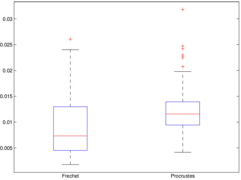
An important choice is thus the calibration of the regularization parameters . To illustrate the benefits of using the smoothed Fréchet mean with an automatic choice of the ’s by GCV, we used replications of model (2.2) with . For each repetition , we have computed an estimator of using the Procrustes mean without smoothing, and an estimator of using a smoothed Fréchet mean where each is chosen by denoising the -th signal by GCV. In Figure 7, we display boxplots (for ) of the mean squared errors
It can be seen that, over replications, the mean squared error of the smoothed Fréchet mean is clearly much lower than the one obtained by Procrustes mean.
3 Application to ECG data analysis
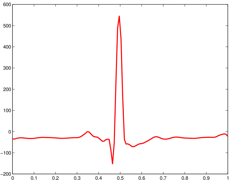
Now, let us return to the analysis of the ECG records displayed in Figure 1. We propose to compare the results obtained by the smoothed Fréchet mean using either translation operators or non-rigid operators given by the family of parametric diffeomorphisms of described in Section 2.4. The smoothing of the signals obtained after segmentation of the ECG records is done by wavelet thresholding with a data-based choice of the regularization parameters as explained in Section 2.2.
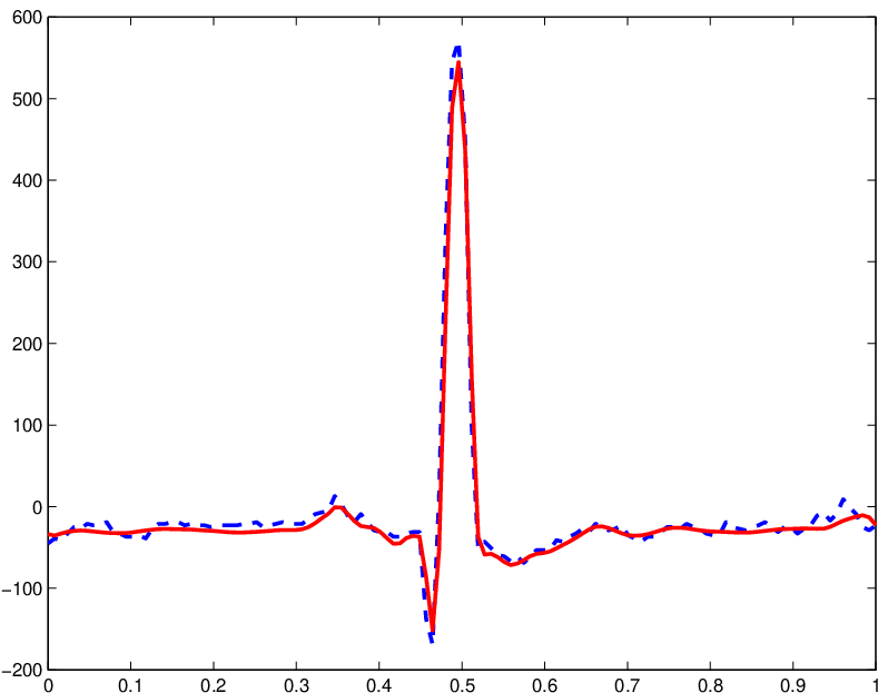
The computation of smoothed Fréchet means using translation operators in the normal and cardiac arrhythmia cases are displayed in Figure 8 and Figure 9. The results obtained using the Procrustes mean are very similar, and they are thus not reported. Note that using Fréchet or Procrustes means with translation operators is very similar to the alignment of signals using cross-correlation which is the widely used technique for signal averaging in ECG data analysis.
One can see that, for the normal case, the results are very satisfactory as the mean heart cycle displayed in Figure 8(a) is a good estimation of the typical shape of the signals displayed in Figure 8(b)-(g). For the case of cardiac arrhythmia, the results are not very satisfactory since there is still a low-pass filtering effect on the shape of the QRS complex (around the time point ) in the mean heart cycle displayed in Figure 9(a). In this case, the Fréchet mean does not represent very well the shape of the signals in Figure 9(b)-(g). This low-pass filtering effect is due to a much larger variability in shape of the signals (after segmentation) in the case of cardiac arrhythmia than in the normal case. Since the activity of the heart can be very irregular in cases of cardiac arrhythmia, modeling shape variability using only translation operators is not flexible enough. A more precise alignment to take into account a local variability in lag and duration of the heart beats is thus needed.
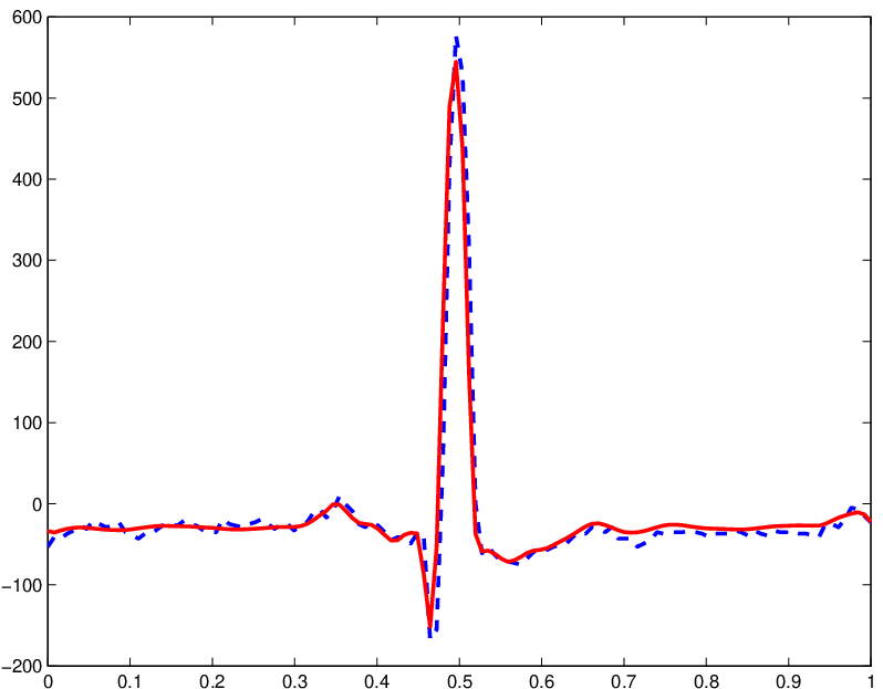
The computation of smoothed Fréchet means using non-rigid operators in the normal and cardiac arrhythmia cases are displayed in Figure 10 and Figure 11. In the normal case, the result is very similar to the one already obtained by the Fréchet mean using translation operators, as shown by the comparison of Figure 8 and Figure 10. In the case of cardiac arrhythmia, the results displayed in Figure 9 and Figure 11 clearly show the improvements obtained by using non-rigid deformation operators. The shape of the mean heart cycle in Figure 11(a) is a better estimation of the typical shape of the signals displayed in Figure 11(b)-(g). In particular, there is no low-pass filtering effect around the time point in the shape of the Fréchet mean.



4 Discussion and conclusion
We have presented a new algorithm for aligning heart beats extracted from an ECG record. Our approach is based on the notion of smoothed Fréchet means of curves using either translation or non-rigid deformation operators. In the case of a normal ECG obtained from a healthy subject, our approach yields a satisfactory mean heart cycle. Note that using Fréchet mean with translation operators is very similar to the computation of a mean heart cycle by aligning the data using cross-correlation which is the widely used approach in ECG data analysis for signal averaging. When using non-rigid operators to align hearts beats having a high shape variability, with peaks showing an important variability in lag and duration from one pulse to another, our approach yields significant improvements over signal averaging by cross-correlation. The benefits of our procedure has been demonstrated for an ECG recording of a subject showing evidence of significant arrhythmia. We hope that the methods presented in this paper will stimulate further investigation into the development of better alignment procedures that take into account local shape variability in heart beats extracted from ECG records.
References
- [ABS01] A. Antoniadis, J. Bigot, and T. Sapatinas. Wavelet estimators in nonparametric regression: A comparative simulation study. Journal of Statistical Software, 6(6):1–83, 6 2001.
- [Afs11] B. Afsari. Riemannian center of mass: existence, uniqueness, and convexity. Proceedings of the American Mathematical Society, 139(2):655–673, 2011.
- [BC11] J. Bigot and B. Charlier. On the consistency of fréchet means in deformable models for curve and image analysis. Electronic Journal of Statistics, 5:1054–1089, 2011.
- [BG10] J. Bigot and S. Gadat. A deconvolution approach to estimation of a common shape in a shifted curves model. Annals of statistics, to be published, 2010.
- [BGL09] J. Bigot, S. Gadat, and J.-M. Loubes. Statistical M-estimation and consistency in large deformable models for image warping. J. Math. Imaging Vision, 34(3):270–290, 2009.
- [Big06] J. Bigot. Landmark-based registration of curves via the continuous wavelet transform. J. Comput. Graph. Statist., 15(3):542–564, 2006.
- [BMTY05] M. F. Beg, M. I. Miller, A. Trouvé, and L. Younes. Computing large deformation metric mappings via geodesic flows of diffeomorphisms. Int. J. Comput. Vision, 61(2):139–157, 2005.
- [CW79] P. Craven and G. Wahba. Smoothing noisy data with spline functions: Estimating the correct degree of smoothing by the method of generalized cross-validation. Numer. Math., 31:377–403, 1979.
- [Fré48] M. Fréchet. Les éléments aléatoires de nature quelconque dans un espace distancié. Ann. Inst. H.Poincaré, Sect. B, Prob. et Stat., 10:235–310, 1948.
- [GAG+13] A. L. Goldberger, L. A. N. Amaral, L. Glass, J. M. Hausdorff, P. Ch. Ivanov, R. G. Mark, J. E. Mietus, G. B. Moody, C.-K. Peng, and H. E. Stanley. PhysioBank, PhysioToolkit, and PhysioNet: Components of a new research resource for complex physiologic signals. Circulation, 101(23):e215–e220, 2000 (June 13). Circulation Electronic Pages: http://circ.ahajournals.org/cgi/content/full/101/23/e215 PMID:1085218; doi: 10.1161/01.CIR.101.23.e215.
- [GH06] A.C. Guyton and J.E. Hall. Textbook of medical physiology. Elsevier Saunders, 2006.
- [GK92] T. Gasser and A. Kneip. Statistical tools to analyze data representing a sample of curves. Annals of Statistics, 20(3):1266–1305, 1992.
- [GK95] T. Gasser and A. Kneip. Searching for Structure in Curve Sample. Journal of the American Statistical Association, 90(432):1179–1188, 1995.
- [GLM07] F. Gamboa, J.-M. Loubes, and E. Maza. Semi-parametric estimation of shifts. Electron. J. Stat., 1:616–640, 2007.
- [Huc11] S. Huckemann. Intrinsic inference on the mean geodesic of planar shapes and tree discrimination by leaf growth. Ann. Statist., 39(2):1098–1124, 2011.
- [KG88] A. Kneip and T. Gasser. Convergence and consistency results for self-modelling regression. Annals of Statistics, 16:82–112, 1988.
- [LJB03] E. Laciar, R. Jané, and D. H. Brooks. Improved alignment method for noisy high-resolution ecg and holter records using multiscale cross-correlation. IEEE Trans. Biomed. Eng., 50(3):344–53, 2003.
- [LM04] X. Liu and H.G. Muller. Functional convex averaging and synchronization for time-warped random curves. Journal of the American Statistical Association, 99(467):687–699, 2004.
- [PT85] J. Pan and W. J. Tompkins. A real-time QRS detection algorithm. IEEE Trans Biomed Eng, 32(3):230–236, 1985.
- [RL01] J.O. Ramsay and X. Li. Curve registration. Journal of the Royal Statistical Society (B), 63:243–259, 2001.
- [RR86a] O. Rompelman and H. H. Ros. Coherent averaging technique: a tutorial review. part 2: Trigger jitter, overlapping responses and non-periodic stimulation. J Biomed Eng, 8(1):30–5, 1986.
- [RR86b] O. Rompelman and H.H. Ros. Coherent averaging technique: a tutorial review. part 1: Noise reduction and the equivalent filter. J. Biomed. Eng., 8(1):24–9, 1986.
- [TIR11] T. Trigano, U. Isserles, and Yaacov Ritov. Semiparametric curve alignment and shift density estimation for biological data. IEEE Transactions on Signal Processing, 59(5):1970–1984, 2011.
- [Vim10] M. Vimond. Efficient estimation for a subclass of shape invariant models. Annals of statistics, 38(3):1885–1912, 2010.
- [WG97] K. Wang and T. Gasser. Alignment of curves by dynamic time warping. Annals of Statistics, 25(3):1251–1276, 1997.
- [You10] L. Younes. Shapes and diffeomorphisms, volume 171 of Applied Mathematical Sciences. Springer-Verlag, Berlin, 2010.