CERN–PH–TH/2011/251 SLAC–PUB–14632 LAPTH-042/11 HU-EP-11/44
Analytic result for the two-loop six-point NMHV amplitude in super Yang-Mills theory
Lance J. Dixon(1), James M. Drummond(2,3)
and Johannes M. Henn(4,5)
(1) SLAC National Accelerator Laboratory,
Stanford University, Stanford, CA 94309, USA
(2) PH-TH Division, CERN, Geneva, Switzerland
(3) LAPTH, Université de Savoie, CNRS,
B.P. 110, F-74941 Annecy-le-Vieux Cedex, France
(4) Humboldt-Universität
zu Berlin, Newtonstraße 15, 12489 Berlin, Germany
(5) Institute for Advanced Study,
Princeton, NJ 08540, USA
lance@slac.stanford.edu , drummond@lapp.in2p3.fr , jmhenn@ias.edu
Abstract
We provide a simple analytic formula for the two-loop six-point ratio function of planar super Yang-Mills theory. This result extends the analytic knowledge of multi-loop six-point amplitudes beyond those with maximal helicity violation. We make a natural ansatz for the symbols of the relevant functions appearing in the two-loop amplitude, and impose various consistency conditions, including symmetry, the absence of spurious poles, the correct collinear behaviour, and agreement with the operator product expansion for light-like (super) Wilson loops. This information reduces the ansatz to a small number of relatively simple functions. In order to fix these parameters uniquely, we utilize an explicit representation of the amplitude in terms of loop integrals that can be evaluated analytically in various kinematic limits. The final compact analytic result is expressed in terms of classical polylogarithms, whose arguments are rational functions of the dual conformal cross-ratios, plus precisely two functions that are not of this type. One of the functions, the loop integral , also plays a key role in a new representation of the remainder function in the maximally helicity violating sector. Another interesting feature at two loops is the appearance of a new (parity odd) (parity odd) sector of the amplitude, which is absent at one loop, and which is uniquely determined in a natural way in terms of the more familiar (parity even) (parity even) part. The second non-polylogarithmic function, the loop integral , characterizes this sector. Both and can be expressed as one-dimensional integrals over classical polylogarithms with rational arguments.
1 Introduction
Much progress has been achieved recently in the analytic understanding of seemingly complicated scattering processes. In particular, attention has been focused on the planar sector, or large limit, of maximally supersymmetric Yang-Mills theory. The scattering amplitudes in this sector of the theory obey many startling properties, which has led to the hope that the general scattering problem might be solvable, exactly in the coupling.
One of the major simplifications that the planar theory enjoys is dual conformal symmetry [1, 2, 3, 4, 5, 6, 7], which dictates how colour-ordered amplitudes behave under conformal transformations of the dual (or region) variables defined via . For the particular case of maximally helicity-violating (MHV) amplitudes, this symmetry is intimately connected to the relation between the amplitudes and Wilson loops evaluated on polygons with light-like edges, whose vertices are located at the [6, 3, 8, 4, 5, 9, 10, 11]. The MHV amplitudes are infrared divergent, just as the corresponding light-like Wilson loops are ultraviolet divergent. The Wilson-loop divergence has the consequence that a suitably-defined finite part transforms anomalously under the dual conformal symmetry [4, 5]. The Ward identity describing this behaviour actually fixes the form of the four-point and five-point amplitudes to all orders in the coupling, to that given by the BDS ansatz [12]. From six points onwards, the existence of dual-conformal invariant cross-ratios means that the problem of determining the MHV amplitude reduces to finding a function that depends only on the cross-ratios — the so-called ‘remainder function’, which corrects the BDS ansatz.
Great advances have been made recently in understanding the form of the remainder function, which is non-trivial beginning at two loops. The need for a two-loop remainder function for Wilson loops was observed for a large number of points in ref. [7], and for six points in ref. [9]. The multi-Regge limit of the six-point scattering amplitude also implied a non-trivial remainder function [13]. At a few generic kinematic points, the Wilson loop [11] and amplitude [10] remainder functions were found to agree numerically. The six-point Wilson loop integrals entering the remainder function were computed analytically in terms of Goncharov polylogarithms [14, 15], and then simplified down to classical polylogarithms [16] using the notion of the symbol of a pure function [17, 18, 19, 16]. The integrals contributing to the six-point MHV scattering amplitude have also been evaluated analytically [20] in a certain kinematical regime using a mass regulator [21], and the remainder function has been found to agree with the Wilson-loop expression of ref. [16]. Very recently, the symbol for the three-loop six-point remainder function was determined up to two arbitrary parameters [22], by imposing a variety of constraints, in particular the operator product expansion (OPE) for Wilson loops developed in refs. [23, 24, 25].
For more than six points, numerical results for the remainder function have been obtained via Wilson loop integrals [26, 27]. Integral representations for the MHV amplitudes have been presented at seven points [28] and for an arbitrary number of points using momentum twistors [29]. Recently, an expression for the symbol of the two-loop remainder function has been given for an arbitrary number of points [30], and the structure of the OPE for this case has been explored [31]. In special kinematics corresponding to scattering in two space-time dimensions, analytic results are available for a number of configurations at two loops [32, 33, 34] and conjecturally even at three loops [35].
When one considers amplitudes beyond the MHV sector, there is another finite dual conformally invariant quantity that one can consider, namely the ‘ratio function’ . This quantity is defined by factoring out the MHV superamplitude from the full superamplitude [36],
| (1.1) |
Infrared divergences are universal for all component amplitudes; hence the MHV factor contains all such divergences, leaving an infrared finite quantity . One of the central conjectures of ref. [36] is that is also dual conformally invariant. There is strong supporting evidence for this conjecture in the form of direct analytic one-loop results [37, 38, 39, 40, 41] and, in the six-point case, numerical evidence at two loops [42]. In this paper, we will construct the ratio function analytically at two loops for six external legs.
At tree level, the ratio function is given by a sum over dual superconformal ‘-invariants’ [36, 43, 44, 45, 46, 47]. These quantities are invariant under a much larger (infinite-dimensional) Yangian symmetry, obtained by combining invariance under both the original and dual copies of superconformal symmetry [48]. Beyond tree level one finds -invariants dressed by dual conformally invariant functions [36, 41, 42]. Since the -invariants individually exhibit spurious poles, which cannot appear in the final amplitude, they cannot appear in an arbitrary way. The particular linear combination appearing in the tree amplitude is free of spurious poles. At loop level, the absence of spurious poles implies restrictions on the dual conformally invariant functions that dress them [49]. Additional restrictions on these same functions come from the known behaviour of the amplitude when two of the external particles become collinear. These constraints will be important in our construction of at two loops.
A consequence of the duality between MHV amplitudes and light-like Wilson loops is that the remainder function can be analysed by conformal field theory methods, such as the operator product expansion (OPE) [23, 24, 25]. Various proposals have been put forward for extending the duality between amplitudes and Wilson loops beyond the MHV sector, either in terms of a supersymmetric version of the Wilson loop [50, 51, 30], or in terms of correlation functions [52, 53]. Although there may be various subtleties in realising such an object, compatible with the full supersymmetry in a Lagrangian formulation [54], one may instead justify the existence of such an object through the OPE. The framework for pursuing this approach was developed in ref. [55], and agreement was found with the known one-loop six-point next-to-MHV (NMHV) amplitude [37, 39, 40, 41]. This agreement provides non-trivial evidence that there does indeed exist a Wilson-loop quantity dual to all scattering amplitudes.
The aim of this paper is to combine various approaches in order to determine the six-point ratio function , or equivalently the NMHV amplitude, analytically at two loops. This quantity was expressed in terms of dual conformal integrals, and computed numerically, in ref. [42]. We proceed in a manner similar to our recent examination of the three-loop six-point remainder function [22]. In particular, we make an ansatz for the symbols of the various pure functions involved. (See appendix A for a brief introduction to pure functions and their symbols.) In other words, we assume that the functions that appear fall within a particular class of multi-dimensional iterated integrals, or generalized polylogarithms. We say functions rather than function because in general, beyond one loop, one can imagine that there are both (parity even)(parity even) and (parity odd)(parity odd) contributions, in a sense which we make specific in the next section. For convenience, we call these contributions ‘even’ and ‘odd’, respectively. At tree level and at one loop, the odd part vanishes.
After constructing an ansatz, the next step is to impose consistency conditions. We first impose the spurious pole and collinear conditions. Then we impose that a certain double discontinuity is compatible with the OPE [23, 24, 25, 55]. At this stage, we find that the symbols for the relevant functions contain nine unfixed parameters. We convert these symbols into explicit functions. In general, this step leads to ‘beyond-the-symbol ambiguities’. These ambiguities are associated with functions whose symbols vanish identically, namely transcendental constants, such as the Riemann values , multiplied by pure functions of lower degree. However, in the present case, after re-imposing the spurious and collinear restrictions at the level of functions, there is only one additional ambiguity, associated with adding the product of with the one-loop ratio function. This term obeys all constraints by itself and has vanishing symbol. We are thus left with a ten-dimensional space of functions. In particular, we find that the odd part is necessarily non-zero. Moreover, it is uniquely determined in terms of the even part.
In order to fix the remaining free parameters, we turn to a representation of the even part of the two-loop six-point NMHV amplitude based on loop integrals [42]. We analyse this representation, appropriately rewritten with a mass regulator [21], in the symmetric regime with all three cross-ratios equal to . In this regime, the most cumbersome double-pentagon integrals can be traded for the MHV remainder function, plus simpler integrals. This observation allows us to perform an analytic expansion for small and large . Comparing these expansions with the ansatz, we are able to match them, precisely fixing all remaining free parameters. The fact that the ansatz agrees with the expansion of the loop-integral calculation in this regime is a highly non-trivial cross check, since an entire function is matched by an ansatz with just a few free parameters. Further confirmation that our result is correct comes from comparing with a numerical evaluation [42] at a particular asymmetric kinematical point. This latter check also confirms the expectation that is defined independently of any infrared regularization scheme. See also ref. [56] for a recent discussion of different infrared regularizations and regularization-scheme independence.
In contrast to the the two-loop six-point MHV amplitude [16], the two-loop six-point ratio function cannot quite be expressed in terms of classical polylogarithms. Two additional functions appear, one in the even part and one in the odd part. However, these functions have a very simple structure: we can write them as simple one-dimensional integrals over classical polylogarithmic functions of degree three. The even part of the ratio function can be written in terms of single-variable polylogarithmic functions whose arguments are rational in the three cross-ratios , plus one of the new functions, which coincides with the finite double-pentagon integral [57]. We use the differential equations obeyed by this integral [58, 59] to derive various parametric integral representations for it. The odd part consists entirely of the second new function, , which also can be expressed as a single integral over classical polylogarithms of degree three. This function can also be identified as the odd part of another finite double-pentagon integral, [57], which we compute using the differential equations derived in ref. [58].
This paper is organized as follows. In section 2 we review non-MHV amplitudes, and the definition of the ratio function in planar super Yang-Mills theory. We discuss the physical constraints satisfied by , namely in the collinear and spurious limits, and also those arising from the OPE expansion of super Wilson loops. We make an ansatz for the symbol of at two loops in section 3, and then apply the constraints. In order to promote the symbol to a function, we introduce in section 4 two new functions that are not expressible in terms of classical polylogarithms, but have simple parametric integral definitions. Next, in section 5, we parametrise the beyond-the-symbol ambiguities and apply the collinear and spurious constraints at the functional level, which leaves only ten unfixed parameters. In section 6 we determine these parameters by performing an analytic two-loop evaluation of the integrals contributing to the even part of the NMHV amplitude in a special kinematical regime. The final result for the full two-loop NMHV ratio function is presented in section 7. We conclude in section 8. Several appendices contain background material and technical details. We provide the symbols for several of the quantities appearing in this article as auxiliary material.
2 Non-MHV amplitudes and the ratio function
To describe the scattering amplitudes of super Yang-Mills theory, it is useful to introduce an on-shell superspace (see e.g. refs. [60, 61, 36, 62]). All the different on-shell states of the theory can be arranged into an on-shell superfield which depends on Grassmann variables transforming in the fundamental representation of ,
| (2.1) |
Here , , , , and are the positive-helicity gluon, gluino, scalar, anti-gluino, and negative-helicity gluon states, respectively. These on-shell states carry a definite null momentum, which can be written in terms of two commuting spinors, . Note that the spinors and are not uniquely defined, given ; they can be rescaled by , . The transformation properties of the states and the variables are such that the full superfield has weight 1 under the following operator,
| (2.2) |
All the different (colour-ordered) scattering amplitudes of the theory are then combined into a single superamplitude , from which individual components can be extracted by expanding in the Grassmann variables associated to the different particles. The tree-level MHV superamplitude is the simplest cyclically invariant quantity with the correct scaling behaviour for each particle that manifests translation invariance and supersymmetry,
| (2.3) |
The arguments of the delta functions are the total momentum and total chiral supercharge , respectively. The full MHV superamplitude is the tree-level one multiplied by an infrared-divergent factor,
| (2.4) |
Moving beyond MHV amplitudes, we define the ratio function by factoring out the MHV superamplitude from the full superamplitude [36],
| (2.5) |
Here has an expansion in terms of increasing Grassmann degree, corresponding to the type of amplitudes (MHV, NMHV, N2MHV, etc.),
| (2.6) |
The number of terms in the above expansion of is , where is the number of external legs. The Grassmann degrees of the terms are . At six points, which is the case of interest for this paper, there are just three terms, corresponding to MHV, NMHV and N2MHV. The N2MHV amplitudes for are equivalent to amplitudes, which are simply related to the MHV amplitudes by parity. Thus the non-trivial content of the ratio function at six points is in the NMHV term.
At tree level, is given by a sum over dual superconformal ‘-invariants’ [36]. In particular, for six points we have
| (2.7) |
The -invariants can be described using dual coordinates , defined by
| (2.8) |
| (2.9) |
The -invariants take an even simpler form in terms of momentum twistors [63, 45]. These variables are (super)twistors associated to the dual space with coordinates . They are defined by
| (2.10) |
The momentum (super)twistors transform linearly under dual (super) conformal symmetry, so that is a dual conformal invariant. The -invariants can then be written in terms of the following structures:
| (2.11) |
which contain five terms in the sum over cyclic permutations of in the delta function. The bracket notation serves to make clear the totally anti-symmetrised dependence on five momentum supertwistors. The quantity is a special case of this general invariant,
| (2.12) |
At the six-point level it is clear that there are six different such invariants. We label them compactly by , using the momentum twistor that is absent from the five arguments in the brackets:
| (2.13) |
and so on.
In general -invariants obey many identities; see for example refs. [36, 41]. These identities can be organised as residue theorems in the Grassmannian interpretation [44]. At six points, the only identity we need is [36]
| (2.14) |
Using eqs. (2.12), (2.13) and (2.14), we can rewrite the NMHV tree amplitude (2.7) as
| (2.15) |
Beyond tree level, the -invariants in the ratio function are dressed by non-trivial functions of the dual conformal invariants [36]. In the six-point case, there are three independent invariants. We may parametrise the invariants by the cross-ratios,
| (2.16) |
Often it will also be useful to use the variables defined by,
| (2.17) |
where
| (2.18) |
In terms of momentum twistors, the cross-ratios are expressed as
| (2.19) |
while the variables simplify to
| (2.20) |
In this form, it is clear that a cyclic rotation by one unit maps the variables as follows,
| (2.21) |
while the cross-ratios behave in the following way,
| (2.22) |
The parity operation which swaps the sign of the square root of (i.e. inverts the variables) is equivalent to a rotation by three units in momentum twistor language. Indeed one can think of the cross-ratios as independent, parity-invariant combinations of the variables. Specifically we have
| (2.23) |
and similar relations obtained by cyclic rotation. Because of the ambiguity associated with the sign of the square root of in eq. (2.17), the primary definition of the variables is through the momentum twistors and eq. (2.20). Further relations between these variables are provided in appendix F.
At six points it can also be convenient to simplify the momentum-twistor four-brackets by introducing [16] antisymmetric two-brackets of variables via [53]
| (2.24) |
so that we have
| (2.25) |
plus six more relations obtained by cyclic permutations.11 1 In comparison with ref. [22], the indexing of the variables differs by one unit, and a square-root ambiguity in defining the variables was resolved in the opposite way.
Having specified our notation for the invariants we need, we now parametrise the six-point NMHV ratio function in the following way,
| (2.26) |
The and are functions of the conformal invariants and of the coupling, with the even under parity while the are odd (recall that parity is equivalent to a rotation by three units). The cyclic and reflection symmetries of the amplitude (and hence the ratio function ) mean that the and are not all independent. Indeed, choosing and , we can write
| (2.27) |
The functions and obey the symmetry properties,
| (2.28) |
Note that we have written the parity-odd function as a function of the variables, while , being parity even, can be written as a function of the cross-ratios. The functions and depend on the coupling. We expand them perturbatively as follows,
| (2.29) |
Here
| (2.30) |
where is the Yang-Mills coupling constant for gauge group ; the planar limit is with held fixed.
At tree level, we have while vanishes. One can see that the expression (2.27) with agrees with eq. (2.15). At one loop, still vanishes, while is a non-trivial function involving logarithms and dilogarithms,
| (2.32) |
The main results of this paper are analytical two-loop expressions for and , both of which are non-vanishing.
Let us discuss some general constraints that the functions and obey.
Physical poles in amplitudes are associated with singular factors in the denominator involving sums of color-adjacent momenta, of the form . In the -invariants, in the notation of eq. (2.11), such poles appear as four brackets of the form
| (2.33) |
However, the -invariants also contain spurious poles, which arise from the four brackets that are not of this form. The full amplitude must not have such poles. Therefore the functions and must conspire to cancel the pole with a zero in the corresponding kinematical configuration.
In the dual-coordinate notation (2.9), the -invariants contain poles from denominator factors of the form . For special values of , such factors can simplify into physical singularities, but for generic values they correspond to spurious poles. In the six-point case, for example, contains a factor of
| (2.34) |
in the denominator. While the pole at is a physical (collinear) singularity, the pole at is spurious. In momentum-twistor notation, the spurious pole comes from any four-bracket in the denominator which is not of the form .
For example, in the six-point case the -invariants and both contain the spurious factor in the denominator. (In the dual-coordinate notation, this particular pole is proportional to rather than .) In the tree-level amplitude (2.15) there is a cancellation between the two terms, so we see that
| (2.35) |
At loop level, using this relation, we find that the absence of the spurious pole implies the following condition on and ,
| (2.36) |
As the spurious bracket vanishes, we find the following limiting behaviour,
| (2.37) |
This is easiest to see in the two-bracket notation of eq. (2.24), in which corresponds to and hence to . The above condition reduces to the one of ref. [49] on the assumption that .22 2 This is true after correcting a typo in eq. (3.63) of that reference. The one-loop expression for , eq. (), satisfies the above constraint with , since in the limit.
There is also a constraint from the collinear behaviour. There are two types of collinear limits, a ‘-preserving’ one where NkMHV superamplitudes are related to NkMHV superamplitudes with one fewer leg, and a ‘-decreasing’ one which relates NkMHV superamplitudes to Nk-1MHV superamplitudes with one fewer leg. These two operations are related to each other by parity and correspond to a supersymmetrisation of the two splitting functions found when analysing pure gluon amplitudes [64, 65, 37, 66, 42]. For the six-point NMHV case, we only need to examine one of the collinear limits; the other will follow automatically by parity.
Under the collinear limit, the -point amplitude should reduce to the -point one multiplied by certain splitting functions. The splitting functions are automatically taken care of by the MHV prefactor in eq. (2.5). The -point ratio function should then be smoothly related to the -point one. Consequently, in the collinear limit the loop corrections to the six-point ratio function should vanish, because the five-point ratio function (containing only MHV and components) is exactly equal to its tree-level value. The -invariants behave smoothly in the limit, either vanishing or reducing to lower-point invariants. In the case at hand we can consider the limit , which also corresponds to , or , or with . In this limit, all -invariants vanish except for and , which become equal. Beyond tree level, the sum of their coefficients must therefore vanish in the collinear regime. This implies the constraint,
| (2.38) |
In fact the parity-odd function drops out of this constraint. The reason is that the collinear regime can be approached from the surface (see eq. (2.18)), and all parity-odd functions should vanish on this surface.
The final constraint we will need comes from the predicted OPE behaviour of the ratio function [55]. The general philosophy that an operator product expansion governs the form of the amplitudes comes from the relation of amplitudes to light-like Wilson loops. Light-like Wilson loops can be expanded around a collinear limit and the fluctuations can be described by operator insertions inside the Wilson loop [23, 24, 25]. By extending this philosophy [55] to supersymmetrised Wilson loops [51, 50] (or equivalently correlation functions [52]) one can avoid questions about giving a precise Lagrangian description of the object under study. In this sense the OPE can be used to justify the existence of a supersymmetrised object dual to non-MHV amplitudes.
The analysis of ref. [55] allows one to choose various components of the ratio function. Let us consider the component proportional to . The only term in eq. (2.27) that contributes to this component is the first one,
| (2.39) |
In order to examine the OPE, we follow ref. [55] and choose coordinates by fixing a conformal frame where
| (2.40) |
and the three cross-ratios are given by
| (2.41) |
Extrapolating the results of ref. [55] to two loops, the OPE predicts the leading (double) discontinuity of the component of the ratio function to be,
| (2.42) |
where
| (2.43) | ||||
| (2.44) | ||||
| (2.45) |
Here is the hypergeometric function, is the Euler beta function, and is the logarithmic derivative of the function.
3 Ansatz for the symbol of the two-loop ratio function
In order to make a plausible ansatz for the ratio function at two loops we assume that the functions and are pure functions of , and , i.e. iterated integrals or multi-dimensional polylogarithms of degree four. Moreover, we make an ansatz for the symbols of and , requiring that their entries are drawn from the following set of nine elements,
| (3.1) |
We summarise some background material on pure functions and symbols in appendix A. We recall that the variables invert under parity. The parity-even function should have a symbol which contains only terms with an even number of entries. Likewise the symbol of the parity-odd function should contain only terms with an odd number of entries. The ansatz for the symbol entries is the same as the one used recently for the three-loop remainder function [22] (after omitting restrictions on the final entry of the symbol). It is consistent with every known function appearing in the six-point amplitudes of planar super Yang-Mills theory, in particular the simple analytic form of the two-loop remainder function found in ref. [16]. It is also consistent with the results for explicitly known loop integrals appearing in such amplitudes, see refs. [58, 59, 67]. In the ensuing analysis we will find many strong consistency checks on our ansatz.
Let us pause to note that our assumption that the relevant functions are pure functions of a particular degree equal to twice the loop order is by no means an innocent one. Although it is true that such general polylogarithmic functions generically show up in amplitudes in four-dimensional quantum field theories, it is certainly not true in general that they always appear with a uniform degree dependent on the loop order. In QCD, for example, the degrees appearing range from twice the loop order to zero, and the transcendental functions typically appear with non-trivial algebraic prefactors. In fact the observed behaviour of having maximal degree only is limited to super Yang-Mills theory, and the most evidence is for the planar sector. This behavior is the generalization, to non-trivial functions of the kinematics, of the maximal degree of transcendentality for harmonic sums that has been observed in the anomalous dimensions of gauge-invariant local operators [68].
The symbols we construct from the set of letters (3.1) should obey certain restrictions. They should be integrable; that is, they should actually be symbols of functions. The initial entries of the symbol should be drawn only from the set , because the leading entry determines the locations of branch points of the function in question, and branch integrable symbols of degree 4 for , and 2 for , obeying the initial entry condition as well as the symmetry conditions (2.28). The spurious pole conditions (2.36) provide 14 constraints and the collinear conditions (2.38) provide 14 more, leaving 15 free parameters at this stage. In order to impose the constraints from the leading discontinuity predicted by the OPE, we use the fact that the sum (2.42) is annihilated by the following differential operator [55],
| (3.2) |
In the variables this differential operator is given by
| (3.3) |
where
| (3.4) |
Imposing that the double discontinuity (2.39) is annihilated by the operator gives 5 further conditions, leaving 10 free parameters in the symbol. One of these parameters, denoted by below, is just the overall normalisation of the symbol of the double discontinuity, which is non-zero and convention-dependent. In the following we provide functions with physical branch cuts which represent the symbol. We find that the solution has the form,
| (3.5) |
where and through are the constant free parameters, and the quantities , , and will be defined below.33 3 In section 6 we will fix the ten parameters using an analytical computation for particular kinematics. We have compared the symbols (3.5) for and with all parameters fixed to an independent computation of these symbols from a formulation of the super Wilson loop [69]; the results agree precisely.
The double discontinuities of the functions appearing in eq. (3.5) obey
| (3.6) | |||||
| (3.7) | |||||
| (3.8) |
Consistency with the spurious pole condition (2.36) forces the odd part to be non-zero, given that is non-zero. The odd part contains no ambiguity at the level of the symbol (or beyond it), once we fix the even part, particularly the two parameters and .
The symbol of the double discontinuity of and is entirely controlled by , through eq. (3.6). We can find a function compatible with this symbol, and compare it to eq. (2.42) to fix the terms. We find that
| (3.9) | |||||
In order to present the symbols appearing in eq. (3.5) explicitly and compactly, it is very useful to employ harmonic polylogarithms [70, 71, 72]. This presentation simultaneously accomplishes the following step, of turning the symbols into functions, up to certain beyond-the-symbol ambiguities. The functions we will present are of degree at most four, and almost all of them can be represented in terms of classical functions. Thus the use of harmonic polylogarithms may seem unnecessarily complicated. However, it is a very useful way to represent, at any degree, a symbol only involving the letters , whereas functions are often insufficient beyond degree four.
Harmonic polylogarithms are single-variable functions defined by iterated integration. It is very simple to write down their symbols. We use harmonic polylogarithms with labels (weight-vector entries) “0” and “1” only. The symbol of a harmonic polylogarithm of argument is obtained by reversing the list of labels and replacing all “0” entries by and all “1” entries by . Finally, one multiplies by where is the number of “1” entries. For example, the symbol of is , and the symbol of is .
We also use the common convention of shortening the label list by deleting each “0” entry, while increasing by one the value of the first non-zero entry to its right, so that, for example, and . Apart from the logarithm function, we take all arguments of the harmonic polylogarithms to be , or . This representation guarantees that the functions we are using to represent the symbol do not have any branch cut originating from an unphysical point. We then compactify the notation further by writing , and so on. Finally, we recall that the symbol of a product of two functions is given by the shuffle product of the two symbols.
With this notation we can immediately write down a function which has the symbol, , of the part of with non-zero double discontinuity, i.e. the part fixed by the OPE,
| (3.10) |
We can similarly write down functions with the correct symbols for the first seven ambiguities in the even part (the double discontinuity of each function vanishes):
For the even part there remain two more ambiguities whose symbols cannot be expressed in terms of those of the single-variable harmonic polylogarithms with the arguments we have been using,
Here stands for the two-loop remainder function, whose symbol is known [16]. The appearance of the two-loop remainder function as an ambiguity should not be surprising. It is a function with physical branch cuts, which vanishes in the collinear limit. Also, it is totally cyclic and hence automatically satisfies the spurious pole condition on its own. Furthermore, it has vanishing double discontinuities and hence drops out from the leading-discontinuity OPE criterion (2.42). It is known [16] that can in fact be expressed in terms of single-variable classical polylogarithms. However, to do so one must use arguments involving square roots of polynomials of the cross-ratios.
The other quantity not given in terms of the harmonic polylogarithms, which enters , is the integral . In fact its symbol can also be recognised from other considerations [58, 59], as we will discuss in the next section. The symbol of is,
| (3.11) |
where
| (3.12) |
Here is the one-loop six-dimensional hexagon function [59, 67], whose symbol is given explicitly in terms of the letters of our ansatz [59],
| (3.13) |
where is a finite, four-dimensional one-loop hexagon integral [57, 58],
| (3.14) |
The other degree 3 symbols above can be represented by harmonic polylogarithms as follows,
| (3.15) |
For the symbol of the parity-odd function , we find that the part fixed by the OPE (acting in conjunction with the spurious-pole constraint (2.36)), , coincides with the symbol of
| (3.16) |
For the odd part of the ambiguity associated with , we have
| (3.17) |
where the functions are given by,
| (3.18) |
We emphasise again that the formulas presented in this section are meant to represent the symbols of the functions involved. For some of the relevant symbols ( and through ) we were able to trivially write down actual functions which represent those symbols in terms of single-variable harmonic polylogarithms with arguments , where is one of the cross-ratios. For two others ( and ) we recognised them as involving symbols of functions we already know, namely the two-loop remainder function and the one-loop six-dimensional hexagon integral. In order to write down actual functions for and there are two issues to address. Firstly, we must give functions which represent the symbols and . Secondly, we must include all possible terms which have vanishing symbol and which are therefore insensitive to the analysis we have presented so far. We address these two issues in the next two sections.
4 Digression on integral representations for and
Here we will present integral formulas to define the functions and whose symbols are given in the previous section. We also present a new representation of the two-loop remainder function, based on the integral . This section is more technical, and could therefore be skipped on a first reading.
4.1 Integral representations for
We start with the finite double-pentagon integral [57]. Let us take a derivative with respect to . The only contributing term from the symbol (3.11) is the last one, so we see that the symbol is consistent with the differential equation,
| (4.1) |
We recognise here the differential equation [59] relating the two-loop, finite double-pentagon integral to the massless, one-loop, six-dimensional hexagon function .
The relation (4.1) can be used to write an integral formula for ,
| (4.2) |
The relevant boundary condition is , where is the two-loop pentaladder function found in ref. [58]. The boundary behaviour at was tested numerically from the Mellin-Barnes representation for [58]. The symbol (3.11) reduces to the symbol of at . It is the unique symbol within our ansatz, built from the letters in eq. (3.1), that obeys eq. (4.1) and the boundary condition. The integral in eq. (4.2) is well-defined and real in the Euclidean region, i.e. the positive octant in which are all positive, because the integrand is well-defined and real there, and is well-behaved even where vanishes [59].
As discussed in ref. [59], the first-order differential equation (4.1) can be obtained from the second-order equation of ref. [58] for the double-pentagon integral, which can be written as
| (4.3) |
Because the second-order operator naturally factorises into two first-order operators, we can integrate up to in two steps. This procedure will yield another one-dimensional integral relation for . We define
| (4.4) |
so that
| (4.5) |
The above formula can be used to define the function ,
| (4.6) | ||||
This function obeys eq. (4.5) and has a symbol coinciding with that of from eq. (3.15). It also obeys . In principle, eq. (4.5) allows one to add beyond-the-symbol terms to that are proportional to , and to . We verified numerically that these terms are absent. The function is manifestly real in the positive octant.
Given the function , we can integrate eq. (4.4) to obtain . We first note that the relevant operator becomes very simple in the variables,
| (4.7) |
Inserting this relation into eq. (4.4), we find an alternative integral formula for in terms of the variables,
| (4.8) |
Here we use the notation . Note that this integral is well-defined at the lower limit of integration, for the following reason: Whenever the product of the variables is unity, , we see from eq. (2.23) that the cross-ratios collapse to the point , and at that point vanishes, . Equation (4.8) can be applied straightforwardly in the variables for and , and also for and . (In other regions, the vicinity of makes a direct integration problematic.)
It can be more convenient to map the integral (4.8) back to the space. This mapping avoids problems related to the variables becoming complex when is negative. To do this mapping, we first define
| (4.9) | |||||
| (4.10) | |||||
| (4.11) |
Notice that and are actually independent of . Therefore the curve of integration in the integral (4.8) from to , which has constant and , should have a constant value of and along it, while varies. Also,
| (4.12) |
so that the measure in eq. (4.8) is just .
Let be the values of along the curve from to . We solve the two constraints, that and are constant along the curve, i.e.
| (4.13) | |||||
| (4.14) |
for and in terms of , obtaining,
| (4.15) | |||||
| (4.16) |
Inserting these expressions into , we have
| (4.17) |
which enables us to use as the final integration parameter,
| (4.18) |
Using this formula, with from eq. (4.6), for which the polylogarithms are all rational functions of the cross ratios, it is easy to rapidly get high-accuracy values for . For example, we find
| (4.19) | |||||
| (4.20) | |||||
| (4.21) |
in general agreement with the numbers obtained at these points using a Mellin-Barnes representation for the loop integral.
4.2 A new representation of the two-loop remainder function
Now that we have obtained representations of the function , we note that the two-loop remainder function can be written in terms of this function, together with functions with purely rational (-independent) symbols. Specifically, we have
| (4.22) |
The piece with a rational symbol is defined as
| (4.23) |
with
| (4.24) |
The function is real when all three cross-ratios are positive. Almost all of the terms in eqs. (4.23) and (4.24) make this manifest term-by-term, because they contain only logarithms of cross-ratios, or for some argument which is less than one. The one slight exception is the combination
| (4.25) |
It is easy to see that eq. (4.25) is real as well, but in this case the branch cut starting at in each term cancels in the sum.
In one sense, the representation (4.22) is a step backward from ref. [16], because the function cannot be expressed in terms of classical polylogarithms, whereas can be. (The absence of a classical polylogarithmic representation for can be seen from its symbol, using the test described in ref. [16].) However, the appearance of the sum over cyclic permutations of the finite two-loop double-pentagon integral is natural, and the coefficient of matches the one in the expression for the two-loop MHV amplitude in ref. [57]. The relation (4.22) between and will be useful for us in the ensuing NMHV analysis.
4.3 An integral representation for
We can obtain in a similar way an integral formula for the parity-odd function . Note that we already have a formula, eq. (3.16), for the function . It is useful to observe that the combination has a symbol which can be arranged so that the final entries are drawn from the list,
| (4.26) |
In terms of the variables, the last final entry in the list above is independent of ,
| (4.27) |
This fact allows us to obtain the symbol of the logarithmic derivative with respect to , which is independent of the variables,
| (4.28) | |||||
The combination can then be written as an integral of a function with this symbol,
| (4.29) |
Here is to be considered as a function of the variables for the integration, but it is most simply expressed in terms of the variables ,
| (4.30) | |||||
in which form it is manifestly real in the positive octant.
Using the same trick we used for , we can rewrite the integral (4.29) directly in the space. The only difference is that the roles of and are swapped, and there is an extra factor multiplying the pure function, corresponding to
| (4.31) |
Thus we get,
| (4.32) | |||||
| (4.33) |
where
| (4.34) | |||||
| (4.35) |
The second form of the integral, eq. (4.33), makes clear that in the positive octant, is real for , and pure imaginary for . The overall sign of eq. (4.33) corresponds to the branch of defined in term of the variables in eq. (F.8); it ensures that the logarithmic derivative with respect to reproduces .
5 Ansatz and constraints at function level
Now that we have obtained explicit functions representing the symbols in section 3, we proceed to enumerate the additional possible contributions, all of which have vanishing symbol. The ratio function is real-valued in the Euclidean region in which all three cross-ratios are positive. Each of the above functions entering also has this property. Therefore any additional functions that we add to our ansatz must also obey the property. In addition to the parameters , we have the following real-valued parity-even beyond-the-symbol ambiguities:
- •
At the level,
(5.1) - •
At the level,
(5.2) - •
At the level,
(5.3)
If our ansatz is correct, then we expect that the parity-even function should be given by
| (5.4) |
for some rational values of the and . There are no parity-odd beyond-the-symbol ambiguities that possess only physical branch cuts. (This fact follows from the absence of an integrable parity-odd degree-two symbol whose first slot is constrained to be , or .)
Next we would like to apply the constraint (2.38) from the collinear limit, namely as , , but now at the level of functions, not just symbols. One way to do this is to first complete the functions and into new functions , , each of which gives a vanishing contribution to in the collinear limit. Although the symbols of the functions were already constrained to give a vanishing contribution in this limit, that does not mean that they vanish as functions. Instead we will correct and the by appropriate beyond-the-symbol terms, and , which are constructed from the expressions (5.1), (5.2) and (5.3) for suitable values of the constants . The function requires no such correction, because it is the two-loop MHV remainder function, which vanishes in all collinear limits.
To perform this correction, we need to know the collinear limits of the functions and . For all but , these limits are straightforward to compute. The limit of is more complicated to obtain due to the presence of . We compute this limit directly in appendix B. However, we may also observe that in the collinear constraint equation (2.38), only the combination is needed for small . (To see this, we use the symmetry of under exchange of its first two arguments.) This combination appears on the right-hand side of eq. (4.22), evaluated in the limit , , along with and the simpler function . Now the left-hand side of this equation, the two-loop remainder function, vanishes in the limit. Also, , where is the two-loop pentaladder function [58]. Hence the limit of the pair of functions appearing in reduces to evaluating , using eq. (4.23). The explicit formulas for all the required beyond-the-symbol functions and are given in appendix B.
The collinear constraint at the level of functions fixes 7 out of the 9 beyond-the-symbol terms, leaving only the following combinations which have vanishing collinear contributions:
| (5.5) | |||||
| (5.6) |
The function should therefore be given by
| (5.7) |
where and are arbitrary constants.
We can analyse the constraints coming from the spurious pole condition (2.36) in a similar way. The end result of this analysis is that one more beyond-the-symbol ambiguity is fixed, leaving just one such function free. In fact, this is the maximum number of beyond-the-symbol terms we can fix with this analysis, because one can always add multiplied by the one-loop ratio function, , given in eq. (). This product is a linear combination of and , namely , and it automatically satisfies all constraints by itself. Thus the only remaining beyond-the-symbol ambiguity is .
In the next section, we will calculate analytically the loop integrals contributing to the two-loop NMHV amplitude for special kinematics. We will use this information to determine the remaining unfixed parameters, , through , and (one of) and .
6 Analytic calculation using loop integrals
In this section, we will fix the remaining undetermined parameters in our ansatz by computing the ratio function analytically in a certain kinematical regime.
We find it convenient to perform our calculation using a mass regulator [21]. As was reviewed in section 2, the ratio function is infrared finite. Moreover, it should be independent of the regularization scheme used to compute it. We first verify this statement at one loop by re-evaluating the MHV and NMHV six-point amplitudes in the mass regularization. At two loops, we find agreement with previous numerical results [42] obtained using dimensional regularization.
6.1 Review of six-point MHV amplitudes
Recall from section 2 that supersymmetry allows to write any MHV amplitudes to all loop orders as a product of the tree-level amplitude, multiplied by a helicity-independent function. We have
| (6.1) |
where , and is defined in eq. (2.30). The known structure of infrared divergences takes a particularly simple form if we consider , namely [73]
Here is the cusp anomalous dimension [74]. It is given by
| (6.2) |
and we have
| (6.3) | |||||
| (6.4) |
Moreover, the finite part satisfies a dual conformal Ward identity [4, 5], whose most general solution is
| (6.5) |
with
| (6.6) |
The first term on the right-hand side of eq. (6.5) comes from the BDS ansatz [12], and provides a particular solution to the Ward identity. It is given by the one-loop contribution to , multiplied by one quarter of the (coupling-dependent) cusp anomalous dimension . Hence its kinematical dependence is determined by the one-loop result. The second term on the right-hand side of eq. (6.5), the remainder function [10, 11], depends on three conformal cross-ratios, , and . There is no remainder function for four and five points, because non-vanishing conformal cross-ratios only appear starting at six points. The specific choice of the kinematic-independent terms and , determined by the four-point and five-point cases, was made in such a way [12] that vanishes in the collinear limit.
6.2 Six-point NMHV amplitudes and ratio function
The NMHV amplitude can be written as
| (6.7) |
where and . Cyclic symmetry implies that under a cyclic rotation of the external legs, , the permute into each other according to , , , and similarly for the .
We recall from section 2, eq. (2.26), that the ratio function(s) and are defined by [36]44 4 The original definition [36] differs from one used later [42] by a (coupling-dependent) constant. We use the latter definition [42] because it makes the collinear behavior of the simpler. Note that is called in ref. [42].
| (6.8) |
Based on the universality of infrared divergences, and in particular the independence of infrared divergences on the helicity configuration, the ratio function defined in eq. (2.5) is expected to be infrared finite, and independent of the regularization scheme used to compute it. More explicitly, comparing eqs. (6.1), (6.7) and (6.8), we see that
| (6.9) |
Expanding these relations in the coupling constant, we find, at the one- and two-loop orders,
| (6.10) | |||||
| (6.11) | |||||
| (6.12) |
It will be a non-trivial check of our calculation that all infrared divergences cancel in .
6.3 The one-loop ratio function
At one loop, the MHV amplitude is given by [65]
| (6.13) |
where and denotes a permutation of the external momenta. In the NMHV case, we have [37]
| (6.14) |
In writing eqs. (6.13) and (6.14), we converted the corresponding expressions in dimensional regularization to mass regularization. The definitions of the integrals and in this regularization are given in appendix C.
Inserting these results into eq. (6.10) to obtain , and then applying the permutation to get , we recover the expressions for and in eqs. () and (2.32). These results are in perfect agreement with the results of an earlier computation using dimensional regularization [42], confirming the expectation that the ratio function should be independent of the regularization scheme. (The result of the original calculation [36] of the one-loop ratio function differs by a convention-dependent constant.)
6.4 The two-loop ratio function
There exist several representations of and in terms of loop integrals. Using generalized unitarity and dimensional regularization, representations for the loop integrand of and the even part of were found in refs. [10] and [42], respectively. Alternative expressions for a four-dimensional integrand were derived using on-shell recursion relations in refs. [57, 29]. This loop integral representation also describes the odd part . However, it will be convenient for us to choose a form in which the MHV and NMHV amplitudes are treated in a uniform way [10, 42].
As in the one-loop case, we will assume that the loop integrals appearing in the massive regularization are the analogs of those appearing in dimensional regularization [42]. A similar assumption was made for the four-point amplitude up to four loops [75, 73], and for the two-loop MHV amplitudes up to six points [20]. The latter work also required promoting the planar four-dimensional loop integrands of ref. [57] into objects that can be integrated to give a finite result. We should point out that this procedure could in principle miss terms whose integrand vanishes as the mass vanishes, , but that are finite after integration. Although examples of such integrals have been given [73, 76], they have not yet proved relevant in a practical calculation. In principle, there are various ways of introducing mass regulators, which differ in how masses are given to different propagators, leading to different results after integration. We will use the mass regulator of ref. [21], which provides a systematic way of introducing the masses.
We should also comment on ‘-integrals’ present in dimensional regularization, in which numerator factors involve explicit factors of the extra-dimensional components of the loop momentum. These integrals do not seem to have an analog in mass regularization, at least when one neglects terms that vanish as . The -integrals arise in dimensional regularization due to a mismatch in dimension between the four-dimensional external polarization vectors and the -dimensional loop integration variable. It has been observed in explicit computations that in the quantity the -integrals only contribute at in dimensional regularization. At two loops, this requires a cancellation involving one- and two-loop -integrals [10]. Such an interference has no analog, at least through , in the massive regularization, and therefore we drop the -integrals in the dimensionally-regularized integrands of refs. [10] and [42].

At two loops, both the MHV amplitude and the even part of the NMHV amplitude can be parametrized by [42]
| (6.17) | |||||
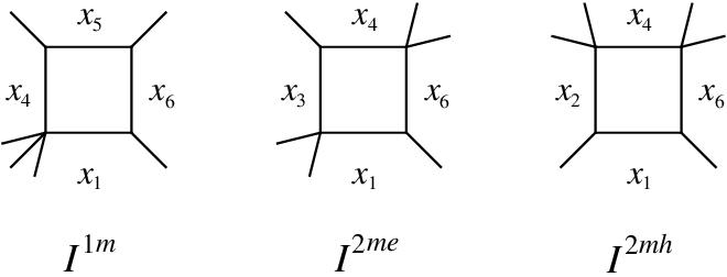
The integrals that enter are depicted in fig. 1. We recall that denotes a rotation of the external momenta by one unit. The coefficients are given by
| (6.18) |
for the MHV case [10], and by
| (6.19) |
for the NMHV case [42]. Here and , with all indices understood to be defined modulo 6.
Then we can write
| (6.20) | |||||
| (6.21) |
In refs. [10, 42], the dimensionally-regularized version of the above formulas was used to study these amplitudes numerically. In particular, the dual conformal invariance of the remainder and ratio functions was tested. The individual integrals are rather complicated, especially the ones of double-pentagon type, and an analytic formula for them is not known yet.
Let us discuss several strategies that might be used to simplify the calculation.
In ref. [20], the calculation of in the massive regularization was simplified by going from the above integral basis to a more convenient one. In particular, the complicated double-pentagon integrals were replaced by other double-pentagon integrals (plus simpler integrals) that are conceptually and practically easier to evaluate.
Another possibility is to exploit the fact that the ratio function is dual conformally invariant, although the individual integrals contributing to it are not. This fact can be used to simplify the expression for the ratio function, by taking limits that leave the cross-ratios invariant, but simplify the individual integrals. This technique turned out to be very useful in computing the Wilson loops dual to MHV amplitudes [15].
Here we use a trick that relies on the following observation. The ratio between the coefficients and is exactly the same in the MHV and NMHV case — see eqs. (6.18) and (6.19). There is still a small mismatch in those terms when comparing eqs. (6.20) and (6.21), due to the different permutation sums. However, this mismatch disappears if we choose a symmetrical kinematical configuration. We can choose, for example,
| (6.22) |
which corresponds to setting all three cross-ratios equal to . As we will see, this kinematical subspace is more than sufficient to fix the remaining ambiguities of the ansatz in the preceding section.
For equal cross-ratios, taking into account the prefactors and different numbers of permutations in eqs. (6.20) and (6.21), we see that the sum of and not only cancels the contributions from and , but cancels or simplifies several other coefficients as well. We can write
| (6.23) |
where is defined according to eq. (6.17), with the new coefficients
| (6.24) |
and where we have combined , because the corresponding integrals are equal at the symmetrical point . Given the known analytical result for , we only need to evaluate the integrals for in order to obtain . We could even further simplify the latter integrals using a more convenient integral basis [20, 57, 29], but this turns out not to be necessary for the present purpose.
Taking into account eq. (6.11), we have
| (6.25) |
Let us collect the relevant formulas here, using in particular eqs. (C.10) and (C.11), and letting :
| (6.26) | |||||
| (6.27) | |||||
| (6.28) | |||||
| (6.29) |
We wish to emphasize that all terms appearing on the right-hand side of eq. (6.25) have infrared divergences in the form of powers of , and that those terms must cancel in the infrared-finite quantity . This cancellation is a non-trivial check of our calculation.
The evaluation of the loop integrals proceeds in the standard way. We give a detailed example in appendix D. We derived Mellin-Barnes representations for all integrals, and then used the Mathematica code MBasymptotics.m [77, 78, 79] in order to perform the asymptotic limit. In this way we could verify the cancellation of the infrared divergent terms, analytically at the level, and numerically at the level. The remaining finite terms are given by at most four-fold Mellin Barnes integrals, which gives us a convenient way of evaluating numerically.
We can do better and use MBasymptotics.m another time in order to compute analytically the small and large limits of . Having in mind that we want to fix the remaining undetermined coefficients of our ansatz from section 3, we go beyond the logarithmic terms in the expansion and also keep power suppressed terms in .
To promote these asymptotic limits back to a full function, we make the analog of the ansatz of section 3, by reducing the result of section 5 to the case of all cross-ratios equal. Hence we expect to be given by a linear combination of and single-variable harmonic polylogarithms.
We can then compare the asymptotic limits we computed against the corresponding expansions of our ansatz. In fact, when fitting a complete function against just a few parameters it is highly non-trivial that we do find a solution. From comparing the first terms in the small and large expansion (see appendix D for more details), we find
| (6.30) | |||||
We also performed numerical checks of this expression at intermediate values of . By comparing eq. (6.30) for with our ansatz (5.7) for and , we find that the remaining twelve parameters in the joint ansatz for and are all fixed. (As mentioned in section 5, there is one additional constraint from the beyond-the-symbol spurious-pole constraint, which is compatible with this solution.) The values of the parameters are,
| (6.31) |
We present the final form of the functions and in the next section.
7 The final formula for the two-loop ratio function
Now we insert the values of the twelve parameters that were fixed in the previous section into our ansatz, and convert everything except and into classical polylogarithms whose arguments are simple, rational functions of , and . The result is
| (7.1) |
where
| (7.2) | |||||
and
| (7.3) | |||||
The function can be evaluated as a simple one-dimensional integral over classical polylogarithms with rational arguments, using eqs. (4.6) and (4.18) from section 4. The function is the two-loop remainder function. It can be expressed entirely in terms of classical polylogarithms whose arguments involve square-root functions of the cross ratios [16]. Alternatively, it can be expressed, using eq. (4.22), in terms of three cyclic permutations of , plus classical polylogarithms with rational arguments. It is clear from eqs. (7.2) and (7.3) that is real in the positive octant, given that and are.
For the odd part we find, using ,
| (7.4) |
This is exactly the linear combination of and (multiplied by an overall ) for which we derived a simple parametric integral formula in section 4.

We can give an alternative form of the final answer that involves both and the double-pentagon integral with ‘mixed’ numerator, [57], where the latter integral is evaluated in appendix E. Due to the respective symmetry and antisymmetry of and under exchange of their first and third arguments, eq. (2.28), the NMHV ratio function is entirely specified by . We have
| (7.5) |
where is implicitly defined by eqs. (4.22), (7.1) and (E.7). Explicitly it is given by,
| (7.6) |
where
| (7.7) | |||||
and
| (7.8) | |||||
We see that is given by sums of products of logarithms and polylogarithms with arguments which are rational combinations of . In other words, the most complicated piece of is captured by the two double-pentagon integrals on the right-hand side of equation (7.5).
Moreover, the only term containing parity-odd pieces on the right-hand side of (7.5) is . We can easily project out the parity-even piece by taking a linear combination of this integral minus the same integral rotated by three steps in the twistor variables. This means that we have an extremely simple representation of the parity-odd function in terms of finite, dual conformal loop integrals (see fig. 2),
| (7.9) |
The same double-pentagon integral with mixed numerator appears in the representation of the NMHV loop integrand that was given in Table 1 of ref. [57]. The latter integral contains both an even and an odd part, although it is not immediately obvious how to separate the two. For example, although the penta-box integrals appearing in the representation of ref. [57] of that amplitude contain odd parts, it can be shown that the latter are only when the integrals are evaluated using a massive regulator [21]; see ref. [20].
We can perform a numerical check of our result for the (parity-even) (parity-even) part. Using the values obtained for in eqs. (4.19), (4.20) and (4.21), we find that
| (7.10) | |||||
| (7.11) | |||||
| (7.12) |
in agreement with the values given in Table I of ref. [42], to the numerical accuracy given there. For reference, we also give the value of , which is the same for all three points due to its symmetry,
| (7.13) |
We also give the numerical values of the parity-odd function at these three points. Here we have to specify the values, or equivalently the branch of the square root of that we consider. At the three points, is negative, . We take the positive imaginary branch of the square root, in defining the values through eq. (2.17). We then evaluate eqs. (4.33) and (7.4) to obtain,
| (7.14) | |||||
| (7.15) | |||||
| (7.16) |
Note that these three values sum to zero.
In fact, although it is not apparent from the integral form (4.33), for general kinematics the function obeys
| (7.17) |
This relation is a consequence of our ansatz and the symmetry condition (2.28). Given this symmetry condition, eq. (7.17) means that the totally antisymmetric part of vanishes. Even if there had existed functions within our ansatz with a totally antisymmetric part, we could have removed them simply by noting that they never contribute to the ratio function (2.27), due to the condition (2.14).
In an auxiliary plain text file accompanying this article, we provide the degree-four symbols for the functions , , , , and . In these files, a term is written as SB.
8 Conclusions and outlook
In this paper we have obtained the full analytic result for the two-loop ratio function in planar super Yang-Mills theory. Our method assumed the existence of two pure functions, and , characterizing the ratio function, and was based on making an ansatz for the letters entering their symbols. We then further restricted the ansatz by imposing physical constraints, such as the behaviour in collinear and spurious regimes, and constraints coming from the operator product expansion of Wilson loops, leaving only a small number of undetermined parameters. The remaining parameters were fixed by an analytic computation of the loop integrals that contribute to the ratio function in particular kinematical regions.
We analysed the constraints in the collinear and spurious pole limits. It is interesting that the spurious pole constraint involves both the (parity-even) (parity-even) and the (parity-odd) (parity-odd) part of the ratio function. We found that, within our ansatz, the (parity-odd) (parity-odd) part is uniquely fixed by the (parity-even) (parity-even) part. In particular, it is necessarily non-zero.
We were able to express the ratio function in terms of sums of products of classical polylogarithms of rational arguments, plus two relatively simple new functions. The first is the parity-even double-pentagon integral . The second is a new function describing the parity-odd sector, but it is also related to the parity-odd part of a second double-pentagon integral, . Neither of these two additional functions can be expressed in terms of classical polylogarithms; however, we have provided simple parametric integral formulas for them, based on the differential equations that the integrals obey. We have checked our result for the (parity-even) (parity-even) part of the ratio function by an analytic two-loop computation (in a special kinematical regime) performed in the present paper, as well as against numerical values in the literature.
Let us comment on the class of functions that can appear within our ansatz. We considered symbols that are built from the set of nine letters , with the physical constraint that the first entry should be drawn from the set only, to exclude non-physical branch cuts. At degrees 1, 2, 3 and 4 there are 3, 9, 25 and 69 integrable parity-even symbols of this kind. At degree 3 and 4 there are also 1 and 6 parity-odd integrable symbols. respectively. As a byproduct of our analysis, we have a complete basis of functions corresponding to the parity-even symbols through degree four, without imposing any symmetries or collinear or spurious pole constraints. Three of the degree-four functions are given by in its three orientations, while the remaining functions are simple sums of products of single-variable harmonic polylogarithms, such as . The labels and the argument are chosen such that only a physical branch cut starting from is present. In general the labels can be any combination of zeros and ones, provided that the last label is 1. The unique parity-odd function at degree three is just the (rescaled) six-dimensional hexagon integral , whose relevance for scattering amplitudes in super-Yang-Mills theory was suggested earlier [59]. The six parity-odd functions at degree four are the three functions , and ; two more functions are given by in two orientations (which is also described by the parity-odd part of the two-loop mixed hexagon ); and there is one further function.
Beyond two loops (i.e. for symbols of degree higher than four) new functions can appear, as in the three-loop MHV remainder function [22]. It would be very interesting to find representations for them, analogous to the simple parametric integral representations obtained in this paper.
The ansatz we made for the symbol was motivated by explicit results for loop amplitudes [16, 22] and loop integrals [58, 59]. Another motivation comes from thinking in terms of twistor-space variables. Our ansatz implies that the letters of the symbol factorise into four-brackets of momentum twistors. This seems natural, because for six points (and hence six twistors describing the scattering data) intersections of lines and planes in twistor space always factorise into twistor four-brackets. At any rate, it would be very interesting if one could prove or disprove our ansatz for the six-point remainder function and ratio function at an arbitrary number of loops. If the ansatz is valid to all loop orders for six-point amplitudes in super Yang-Mills theory, then it is an extremely powerful constraint on the matrix of that theory.
Acknowledgments
We are grateful to Simon Caron-Huot for discussions about the symbol of the ratio function. The work of JMH was supported in part by the Department of Energy grant DE-FG02-90ER40542, and that of LJD by the US Department of Energy under contract DE–AC02–76SF00515.
Appendix A Pure functions and symbols
We define a pure function of degree (or weight) recursively, by demanding that its differential satisfies
| (A.1) |
The sum over is finite and are algebraic functions. This recursive definition is for all positive ; the only degree zero pure functions are constants. The definition (A.1) includes logarithms and classical polylogarithms, as well as other iterated integrals, such as harmonic polylogarithms of one [70] or more [80, 81, 72, 82] variables.
The symbol [17, 18, 19] of a pure function is defined recursively with respect to eq. (A.1),
| (A.2) |
If we continue this process until we reach degree 0, we find that is an element of the -fold tensor product of the space of algebraic functions,
| (A.3) |
where . The symbol of a function loses information about which logarithmic branch the function is on. It also does not detect functions that are transcendental constants multiplied by pure functions of lower degree; such functions have zero symbol. The symbol therefore corresponds to an equivalence class of functions that differ in these aspects. Nevertheless, the symbol is extremely useful, because complicated identities between transcendental functions defined by iterated integrals become simple algebraic identities.
If a symbol can be expressed as a sum of terms, and all entries in each term belong to a given set of variables, then we say that the symbol can be factorised in terms of that set of variables. In this paper we have assumed that the pure functions associated with the NMHV six-point ratio function can be factorised in terms of the set (3.1). From the definition of the symbol, a term containing an entry which is a product can be split into the sum of two terms, according to
| (A.4) |
Performing this factorisation is usually necessary to identify all algebraic relations between terms. It is often necessary to perform the step again after taking a kinematic limit, because the algebraic relations in the limit are different than for generic kinematics.
The elements of the symbol are not all independent, but are related by the integrability condition for any function . The integrability relations can be described simply: Pick two adjacent slots in the symbol and replace the corresponding elements by the wedge product in every term. The resulting expression must vanish.
The symbol also makes clear the locations of the discontinuities of the function. If is given by eq. (A.3), then the degree function has a branch cut starting at . The discontinuity across this branch cut, denoted by , is also a pure function, of degree . Its symbol is found by clipping the first element off the symbol for :
| (A.5) |
It is instructive to check, for example, the vanishing of the double discontinuity for the functions in eq. (3.7), by inspecting their symbols. Using is enough to show that through obey this relation. Using and is enough to establish it for , and so on.
Appendix B Details of the collinear limit
We give here beyond-the-symbol completions of the functions obeying the collinear limit constraint. We denote the completed functions by or , where the were given already in the main text. The collinearly-consistent completions of the functions and are simple to calculate. We find that we can choose
| (B.1) | ||||
| (B.2) | ||||
| (B.3) | ||||
| (B.4) | ||||
| (B.5) | ||||
| (B.6) | ||||
| (B.7) | ||||
| (B.8) |
To define , the limit of is required. Analyzing the symbol of , one expects the following behavior as ,
| (B.9) |
From the symbol of we can determine the symbol of the . Therefore, the only ambiguities to be fixed are beyond-the-symbol terms in the , for which we can make an ansatz. Then, we fix the latter by comparing against the asymptotic limit of a Mellin-Barnes representation of . We find,
| (B.10) | ||||
| (B.11) | ||||
| (B.12) |
Here is the Nielsen polylogarithm.
The other limit that is needed in eq. (2.38) can be obtained by the symmetry of in the first two entries,
Using these limits, we can determine a correction to such that satisfies eq. (2.38),
| (B.14) |
We found the following identity helpful,
| (B.15) | |||||
We also have
| (B.16) |
because vanishes in all collinear limits.
Appendix C One-loop integrals in massive regularization
All integrals in our paper are given in the mostly-plus metric, so that the distances are positive in the Euclidean region.
The integrals appearing in the one-loop MHV and NMHV amplitudes are
| (C.1) | |||||
| (C.2) | |||||
| (C.3) |
where we recall that with indices defined modulo , such that in particular . See fig. 3. It is convenient to define the dimensionless functions,
| (C.4) | |||||
| (C.5) | |||||
| (C.6) |
They are given by
| (C.7) | |||||
| (C.8) | |||||
and
| (C.9) | |||||
In the symmetric kinematics (6.22), and neglecting the terms, we have,
| (C.10) | |||||
| (C.11) | |||||
| (C.12) |
Appendix D Description of the two-loop computation
Let us illustrate the analytic computation of the loop integrals by using the pentabox integral of fig. 1. It is defined by
| (D.1) | |||||
where the external dual coordinates are in the order , reading counter-clockwise from the external momentum in the figure. Also, is the dual coordinate for the box, and is the one for the pentagon. We remind the reader that the specific mass assignment in eq. (D.1), in particular the fact that the internal propagator is massless, follows from extended dual conformal symmetry. See refs. [21] and [73] for further explanation.
We proceed by deriving a Mellin-Barnes (MB) representation for this integral. This is done by first introducing Feynman parameters in order to carry out the four-dimensional loop integrations. Subsequently, MB parameters are introduced to factorize the Feynman denominator, after which the Feynman integrals can be done trivially. Experience shows that it is convenient to introduce the MB parameters loop by loop [83]. Very detailed derivations of MB representations for integrals like in eq. (D.1) can be found in appendix A of ref. [73].
In the case of integral , the numerator factor deserves a comment. We choose to treat the latter as an inverse propagator. In doing so, some of the formulas we need to use, such as the Feynman parameter formula, develop spurious divergences. In order to be able to still use these formulas, we work with the analytically continued integral , where the numerator factor is replaced by and the integration measure is changed to . We will do our computation for , where all manipulations are allowed, and take the limit later. The MB representation we find in this way is
| (D.2) | |||||
where . Here the integrations go from to in the complex plane. The real part of the must be chosen such that the arguments of all functions have positive real part. One finds that this is only possible for .
The limit is very similar to the regulator limit in dimensional regularization, with the difference that here we expect a finite result, because the original integral was well-defined for . In order to take the limit, one first has to deform some of the integration contours [83]. This procedure has been implemented in the MB.m Mathematica code [77, 78, 79].
Having removed the auxiliary parameter , we have a valid MB representation for . We can now perform the regulator limit . This again involves deforming the integration contours, such that the real part of the exponent of becomes positive, at which point a Taylor expansion in is possible. We neglect power-suppressed terms in , since we are only interested in the logarithmic infrared divergences and in the finite part. In deforming the contours, one picks up residues from poles of the functions, which can produce powers of . The resulting lower-dimensional integrals are treated in the same way.
In fact, the leading divergent and terms are obtained in this way without any remaining MB integrations. For example,
| (D.3) |
All terms with eventually cancel in the definition of the remainder function. We will therefore focus on the finite terms as . The latter are obtained as at most four-fold MB integrals.
In the main text, we have considered the special kinematical regime in eq. (6.22), in which all three cross-ratios are equal to . It is easy to use the Mathematica codes [77, 78, 79] in order to compute the or limits of analytically. For example, we find, in the small limit,
| (D.4) | |||||
It is straightforward to obtain higher orders in these expansions, either analytically or numerically to high precision, but we refrain from reproducing them here to save space.
Computing the asymptotic expansions of all integrals contributing to in this way, we obtain
| (D.5) | |||||
in the small limit, and
| (D.6) | |||||
in the large limit. We remark that the half-integer powers appearing in eq. (D.4) have cancelled in the sum over all integrals contributing to . Higher-order terms in the expansions can be obtained numerically to great accuracy, but are not displayed for brevity.
Comparing eqs. (D.5) and (D.6) to eq. (6.25), we can fix , or equivalently , within our ansatz. In this way we arrive at eq. (6.30) in the main text.
Appendix E Computation of the mixed numerator integral
Differential equation for
Loop integrals of this type satisfy simple second-order differential equations [58]. The key point is the presence of pentagon subintegrals that are also present in . Following ref. [58], it is easy to see that the latter integral satisfies the differential equation
| (E.2) |
where the (rescaled) one-loop hexagon integral with mixed numerator is defined as
| (E.3) |
It is given explicitly by [29]
| (E.4) |
We note that the integrals and are left invariant by the transformation
| (E.5) |
which implies
| (E.6) |
We make the ansatz that is a pure function, whose symbol’s entries are drawn from the set of nine letters . Within this ansatz, we find that eq. (E.2) has a unique solution obeying the symmetry condition (E.6), integrability, and the first entry condition. The solution involves parity-even as well as parity-odd terms.
Having determined the symbol of from the differential equation (E.2), we now promote it to a function. We find that we can express it as55 5 To avoid confusion, we emphasize that differs from , where denotes a cyclic shift of all twistors by one unit. In fact, we have , and hence .
| (E.7) |
with
| (E.8) |
where
| (E.9) | |||||
with defined in eq. (4.24), and where the beyond-the-symbol ambiguity for a function symmetric in and is given by
| (E.10) |
We can ask how many of the can be determined by the differential equation (E.2). Using the variables from appendix F it is not hard to verify that the only functions appearing in that are annihilated by the differential operator are and . Therefore, 7 out of the 9 coefficients can be determined by plugging eq. (E.7) back into eq. (E.2).
Indeed, using the parametric integrals derived in the main text for and , we can easily verify the differential equation (E.2) numerically. We find
| (E.11) |
We will fix the remaining two free parameters and from boundary conditions that we discuss presently.
Boundary conditions for

Let us discuss appropriate boundary conditions for . Here we can use our previous experience with the integral , which at the integrand level differs from only by the numerator in one of the pentagon subintegrals. In fact, the numerators of the two integrals are given by
| (E.12) | ||||
| (E.13) |
Previously it was observed that the integrands of these two integrals reduce to the integrand of a penta-box integral in the soft limit , or equivalently , as shown in fig. 4 [20]. Unfortunately, the penta-box integral is infrared divergent, so that the limit is more subtle at the level of integrals. However, we can use the fact that the numerator vanishes linearly in the soft limit. Because the explicitly known penta-box integral [20] only has logarithmic divergences, we expect the following boundary condition to hold,
| (E.14) |
Here we have parametrized the soft limit for the cross-ratios by .66 6 There is a slight abuse of notation here since, strictly speaking, should be thought of as a function of the variables. However, in the soft limit, its parity-odd piece vanishes, justifying the use of the variables. We have verified equation (E.14) at the symbol level. In the following we will assume it holds also at the level of functions.
A related observation is that vanishes in cyclically related soft limits,
| (E.15) |
This vanishing can in fact be understood as a property of the pentagon sub-integral. Since contains the same sub-integral as , we expect the same boundary condition to hold, i.e.
| (E.16) |
We find that imposing the two boundary conditions (E.14) and (E.16) fixes all but one of the beyond-the-symbol ambiguities in eq. (E.10),
| (E.17) |
Comparing to eq. (E.11), we see that the two solutions are compatible with each other, which is a non-trivial cross check. Moreover, taken together they uniquely fix all the beyond-the-symbol parameters, and we have finally,
| (E.18) |
Appendix F Useful variables
In this paper, we found it useful to work with several sets of variables. We can express the letters appearing in our symbols in terms of four-brackets of twistors,
| (F.1) | ||||
| (F.2) | ||||
| (F.3) |
Since the twistors are redundant, it can sometimes be useful to have a particular parametrization for them, e.g.
| (F.4) |
with
| (F.5) |
Although the variables are constructed using square roots of the original cross ratios , and , the cross ratios themselves are rational combinations of the variables , and . The explicit relations are,
| (F.6) | ||||
| (F.7) | ||||
| (F.8) |
where we have picked a particular branch of .
References
- [1] J. M. Drummond, J. Henn, V. A. Smirnov and E. Sokatchev, “Magic identities for conformal four-point integrals”, JHEP 0701, 064 (2007), hep-th/0607160.
- [2] Z. Bern, M. Czakon, L. J. Dixon, D. A. Kosower and V. A. Smirnov, “The four-loop planar amplitude and cusp anomalous dimension in maximally supersymmetric Yang-Mills theory”, Phys. Rev. D75, 085010 (2007), hep-th/0610248.
- [3] J. M. Drummond, G. P. Korchemsky and E. Sokatchev, “Conformal properties of four-gluon planar amplitudes and Wilson loops”, Nucl. Phys. B795, 385 (2008), arxiv:0707.0243.
- [4] J. M. Drummond, J. Henn, G. P. Korchemsky and E. Sokatchev, “On planar gluon amplitudes/Wilson loops duality”, Nucl. Phys. B795, 52 (2008), arxiv:0709.2368.
- [5] J. M. Drummond, J. Henn, G. P. Korchemsky and E. Sokatchev, “Conformal Ward identities for Wilson loops and a test of the duality with gluon amplitudes”, Nucl. Phys. B826, 337 (2010), arxiv:0712.1223.
- [6] L. F. Alday and J. M. Maldacena, “Gluon scattering amplitudes at strong coupling”, JHEP 0706, 064 (2007), arxiv:0705.0303.
- [7] L. F. Alday and J. Maldacena, “Comments on gluon scattering amplitudes via AdS/CFT”, JHEP 0711, 068 (2007), arxiv:0710.1060.
- [8] A. Brandhuber, P. Heslop and G. Travaglini, “MHV amplitudes in 4 super Yang–Mills and Wilson loops”, Nucl. Phys. B794, 231 (2008), arxiv:0707.1153.
- [9] J. M. Drummond, J. Henn, G. P. Korchemsky and E. Sokatchev, “The hexagon Wilson loop and the BDS ansatz for the six-gluon amplitude”, Phys. Lett. B662, 456 (2008), arxiv:0712.4138.
- [10] Z. Bern, L. J. Dixon, D. A. Kosower, R. Roiban, M. Spradlin, C. Vergu and A. Volovich, “The two-loop six-gluon MHV amplitude in maximally supersymmetric Yang-Mills theory”, Phys. Rev. D78, 045007 (2008), arxiv:0803.1465.
- [11] J. M. Drummond, J. Henn, G. P. Korchemsky and E. Sokatchev, “Hexagon Wilson loop = six-gluon MHV amplitude”, Nucl. Phys. B815, 142 (2009), arxiv:0803.1466.
- [12] Z. Bern, L. J. Dixon and V. A. Smirnov, “Iteration of planar amplitudes in maximally supersymmetric Yang-Mills theory at three loops and beyond”, Phys. Rev. D72, 085001 (2005), hep-th/0505205.
- [13] J. Bartels, L. Lipatov and A. Sabio Vera, “BFKL Pomeron, Reggeized gluons and Bern-Dixon-Smirnov amplitudes”, Phys. Rev. D80, 045002 (2009), arxiv:0802.2065.
- [14] V. Del Duca, C. Duhr and V. A. Smirnov, “An analytic result for the two-loop hexagon Wilson loop in 4 SYM”, JHEP 1003, 099 (2010), arxiv:0911.5332.
- [15] V. Del Duca, C. Duhr and V. A. Smirnov, “The two-loop hexagon Wilson loop in 4 SYM”, JHEP 1005, 084 (2010), arxiv:1003.1702.
- [16] A. B. Goncharov, M. Spradlin, C. Vergu and A. Volovich, “Classical polylogarithms for amplitudes and Wilson loops”, Phys. Rev. Lett. 105, 151605 (2010), arxiv:1006.5703.
- [17] K. T. Chen, “Iterated path integrals”, Bull. Amer. Math. Soc. 83, 831 (1977).
- [18] F. Brown, “Multiple zeta values and periods of moduli spaces ”, Annales scientifiques de l’ENS 42, fascicule 3, 371 (2009), math/0606419.
- [19] A. B. Goncharov, “A simple construction of Grassmannian polylogarithms”, arxiv:0908.2238.
- [20] J. M. Drummond and J. M. Henn, “Simple loop integrals and amplitudes in 4 SYM”, JHEP 1105, 105 (2011), arxiv:1008.2965.
- [21] L. F. Alday, J. M. Henn, J. Plefka and T. Schuster, “Scattering into the fifth dimension of 4 super Yang-Mills”, JHEP 1001, 077 (2010), arxiv:0908.0684.
- [22] L. J. Dixon, J. M. Drummond and J. M. Henn, “Bootstrapping the three-loop hexagon”, JHEP 1111, 023 (2011), arxiv:1108.4461.
- [23] L. F. Alday, D. Gaiotto, J. Maldacena, A. Sever and P. Vieira, “An operator product expansion for polygonal null Wilson loops”, JHEP 1104, 088 (2011), arxiv:1006.2788.
- [24] D. Gaiotto, J. Maldacena, A. Sever and P. Vieira, “Bootstrapping null polygon Wilson loops”, JHEP 1103, 092 (2011), arxiv:1010.5009.
- [25] D. Gaiotto, J. Maldacena, A. Sever and P. Vieira, “Pulling the straps of polygons”, JHEP 1112, 011 (2011), arxiv:1102.0062.
- [26] C. Anastasiou, A. Brandhuber, P. Heslop, V. V. Khoze, B. Spence and G. Travaglini, “Two-loop polygon Wilson loops in 4 SYM”, JHEP 0905, 115 (2009), arxiv:0902.2245.
- [27] A. Brandhuber, P. Heslop, V. V. Khoze and G. Travaglini, “Simplicity of polygon Wilson loops in 4 SYM”, JHEP 1001, 050 (2010), arxiv:0910.4898.
- [28] C. Vergu, “Higher-point MHV amplitudes in 4 supersymmetric Yang-Mills theory”, Phys. Rev. D79, 125005 (2009), arxiv:0903.3526.
- [29] N. Arkani-Hamed, J. L. Bourjaily, F. Cachazo and J. Trnka, “Local integrals for planar scattering amplitudes”, arxiv:1012.6032.
- [30] S. Caron-Huot, “Superconformal symmetry and two-loop amplitudes in planar 4 super Yang-Mills”, arxiv:1105.5606.
- [31] A. Sever and P. Vieira, “Multichannel conformal blocks for polygon Wilson loops”, arxiv:1105.5748.
- [32] V. Del Duca, C. Duhr and V. A. Smirnov, “A two-loop octagon Wilson loop in 4 SYM”, JHEP 1009, 015 (2010), arxiv:1006.4127.
- [33] P. Heslop and V. V. Khoze, “Analytic results for MHV Wilson loops”, JHEP 1011, 035 (2010), arxiv:1007.1805.
- [34] L. F. Alday, “Some analytic results for two-loop scattering amplitudes”, JHEP 1107, 080 (2011), arxiv:1009.1110.
- [35] P. Heslop and V. V. Khoze, “Wilson loops @ 3-Loops in special kinematics”, JHEP 1111, 152 (2011), arxiv:1109.0058.
- [36] J. M. Drummond, J. Henn, G. P. Korchemsky and E. Sokatchev, “Dual superconformal symmetry of scattering amplitudes in 4 super-Yang–Mills theory”, Nucl. Phys. B828, 317 (2010), arxiv:0807.1095.
- [37] Z. Bern, L. J. Dixon, D. C. Dunbar and D. A. Kosower, “Fusing gauge theory tree amplitudes into loop amplitudes”, Nucl. Phys. B435, 59 (1995), hep-ph/9409265.
- [38] Z. Bern, V. Del Duca, L. J. Dixon and D. A. Kosower, “All non-maximally-helicity-violating one-loop seven-gluon amplitudes in 4 super-Yang-Mills theory”, Phys. Rev. D71, 045006 (2005), hep-th/0410224.
- [39] Y.-t. Huang, “ 4 SYM NMHV loop amplitude in superspace”, Phys. Lett. B631, 177 (2005), hep-th/0507117.
- [40] K. Risager, S. J. Bidder and W. B. Perkins, “One-loop NMHV amplitudes involving gluinos and scalars in 4 gauge theory”, JHEP 0510, 003 (2005), hep-th/0507170.
- [41] J. M. Drummond, J. Henn, G. P. Korchemsky and E. Sokatchev, “Generalized unitarity for 4 super-amplitudes”, arxiv:0808.0491.
- [42] D. A. Kosower, R. Roiban and C. Vergu, “The six-point NMHV amplitude in maximally supersymmetric Yang-Mills theory”, Phys. Rev. D83, 065018 (2011), arxiv:1009.1376.
- [43] J. M. Drummond and J. M. Henn, “All tree-level amplitudes in 4 SYM”, JHEP 0904, 018 (2009), arxiv:0808.2475.
- [44] N. Arkani-Hamed, F. Cachazo, C. Cheung and J. Kaplan, “A duality for the matrix”, JHEP 1003, 020 (2010), arxiv:0907.5418.
- [45] L. Mason and D. Skinner, “Dual superconformal invariance, momentum twistors and Grassmannians”, JHEP 0911, 045 (2009), arxiv:0909.0250.
- [46] N. Arkani-Hamed, F. Cachazo and C. Cheung, “The Grassmannian origin of dual superconformal invariance”, JHEP 1003, 036 (2010), arxiv:0909.0483.
- [47] G. P. Korchemsky and E. Sokatchev, “Superconformal invariants for scattering amplitudes in 4 SYM theory”, Nucl. Phys. B839, 377 (2010), arxiv:1002.4625.
- [48] J. M. Drummond, J. M. Henn and J. Plefka, “Yangian symmetry of scattering amplitudes in 4 super Yang-Mills theory”, JHEP 0905, 046 (2009), arxiv:0902.2987.
- [49] G. P. Korchemsky and E. Sokatchev, “Symmetries and analytic properties of scattering amplitudes in 4 SYM theory”, Nucl.Phys. B832, 1 (2010), arxiv:0906.1737.
- [50] L. Mason and D. Skinner, “The complete planar -matrix of 4 SYM as a Wilson loop in twistor space”, JHEP 1012, 018 (2010), arxiv:1009.2225.
- [51] S. Caron-Huot, “Notes on the scattering amplitude / Wilson loop duality”, JHEP 1107, 058 (2011), arxiv:1010.1167.
- [52] B. Eden, P. Heslop, G. P. Korchemsky and E. Sokatchev, “The super-correlator/super-amplitude duality: Part I”, arxiv:1103.3714.
- [53] B. Eden, P. Heslop, G. P. Korchemsky and E. Sokatchev, “The super-correlator/super-amplitude duality: Part II”, arxiv:1103.4353.
- [54] A. Belitsky, G. Korchemsky and E. Sokatchev, “Are scattering amplitudes dual to super Wilson loops?”, Nucl.Phys. B855, 333 (2012), arxiv:1103.3008.
- [55] A. Sever, P. Vieira and T. Wang, “OPE for super loops”, JHEP 1111, 051 (2011), arxiv:1108.1575.
- [56] J. M. Henn, S. Moch and S. G. Naculich, “Form factors and scattering amplitudes in 4 SYM in dimensional and massive regularizations”, arxiv:1109.5057.
- [57] N. Arkani-Hamed, J. L. Bourjaily, F. Cachazo, S. Caron-Huot and J. Trnka, “The all-loop integrand for scattering amplitudes in planar 4 SYM”, JHEP 1101, 041 (2011), arxiv:1008.2958.
- [58] J. M. Drummond, J. M. Henn and J. Trnka, “New differential equations for on-shell loop integrals”, JHEP 1104, 083 (2011), arxiv:1010.3679.
- [59] L. J. Dixon, J. M. Drummond and J. M. Henn, “The one-loop six-dimensional hexagon integral and its relation to MHV amplitudes in 4 SYM”, JHEP 1106, 100 (2011), arxiv:1104.2787.
- [60] V. P. Nair, “A current algebra for some gauge theory amplitudes”, Phys. Lett. B214, 215 (1988).
- [61] G. Georgiou, E. W. N. Glover and V. V. Khoze, “Non-MHV tree amplitudes in gauge theory”, JHEP 0407, 048 (2004), hep-th/0407027.
- [62] N. Arkani-Hamed, F. Cachazo and J. Kaplan, “What is the simplest quantum field theory?”, JHEP 1009, 016 (2010), arxiv:0808.1446.
- [63] A. Hodges, “Eliminating spurious poles from gauge-theoretic amplitudes”, arxiv:0905.1473.
- [64] M. L. Mangano and S. J. Parke, “Multi-parton amplitudes in gauge theories”, Phys. Rept. 200, 301 (1991), hep-th/0509223.
- [65] Z. Bern, L. J. Dixon, D. C. Dunbar and D. A. Kosower, “One-loop -point gauge theory amplitudes, unitarity and collinear limits”, Nucl. Phys. B425, 217 (1994), hep-ph/9403226.
- [66] D. A. Kosower and P. Uwer, “One-loop splitting amplitudes in gauge theory”, Nucl. Phys. B563, 477 (1999), hep-ph/9903515.
- [67] V. Del Duca, C. Duhr and V. A. Smirnov, “The massless hexagon integral in 6 dimensions”, Phys. Lett. B703, 363 (2011), arxiv:1104.2781.
- [68] A. V. Kotikov, L. N. Lipatov, A. I. Onishchenko and V. N. Velizhanin, “Three-loop universal anomalous dimension of the Wilson operators in 4 SUSY Yang-Mills model”, Phys. Lett. B595, 521 (2004), hep-th/0404092.
- [69] S. Caron-Huot, private communication.
- [70] E. Remiddi and J. A. M. Vermaseren, “Harmonic polylogarithms”, Int. J. Mod. Phys. A15, 725 (2000), hep-ph/9905237.
- [71] T. Gehrmann and E. Remiddi, “Differential equations for two-loop four-point functions”, Nucl. Phys. B580, 485 (2000), hep-ph/9912329.
- [72] T. Gehrmann and E. Remiddi, “Numerical evaluation of harmonic polylogarithms”, Comput. Phys. Commun. 141, 296 (2001), hep-ph/0107173.
- [73] J. M. Henn, S. G. Naculich, H. J. Schnitzer and M. Spradlin, “More loops and legs in Higgs-regulated 4 SYM amplitudes”, JHEP 1008, 002 (2010), arxiv:1004.5381.
- [74] I. A. Korchemskaya and G. P. Korchemsky, “On lightlike Wilson loops”, Phys. Lett. B287, 169 (1992).
- [75] J. M. Henn, S. G. Naculich, H. J. Schnitzer and M. Spradlin, “Higgs-regularized three-loop four-gluon amplitude in 4 SYM: exponentiation and Regge limits”, JHEP 1004, 038 (2010), arxiv:1001.1358.
- [76] J. M. Henn, “Scattering amplitudes on the Coulomb branch of 4 super Yang-Mills”, Nucl. Phys. Proc. Suppl. 205-206, 193 (2010), arxiv:1005.2902.
- [77] M. Czakon, “Automatized analytic continuation of Mellin-Barnes integrals”, Comput. Phys. Commun. 175, 559 (2006), hep-ph/0511200.
- [78] M. Czakon, “ MBasymptotics.m”, http://projects.hepforge.org/mbtools/.
- [79] D. Kosower, “ barnesroutines.m”, http://projects.hepforge.org/mbtools/.
- [80] T. Gehrmann and E. Remiddi, “Two-loop master integrals for 3 jets: the planar topologies”, Nucl. Phys. B601, 248 (2001), hep-ph/0008287.
- [81] T. Gehrmann and E. Remiddi, “Two-loop master integrals for 3 jets: the nonplanar topologies”, Nucl. Phys. B601, 287 (2001), hep-ph/0101124.
- [82] D. Maître, “HPL, a Mathematica implementation of the harmonic polylogarithms”, Comput. Phys. Commun. 174, 222 (2006), hep-ph/0507152, package can be downloaded at http://krone.physik.unizh.ch/maitreda/HPL/.
- [83] V. Smirnov, “Feynman integral calculus”, Springer Verlag (2006).