Spatially fractional-order viscoelasticity, non-locality and a new kind of anisotropy

As it stands, equation (1) does not have the form of a viscoelastic equation of motion. We shall prove that it is equivalent to a generic momentum balance equation $\rho\,\mathrm{D}^{2}\,u=\mathrm{div}\,\mathrm{D}\,\upsigma$, where the stress $\upsigma$ is given by the constitutive equation

$$\upsigma=g(t)\ast_{t}\mathbf{C}\,\mathrm{D}\,\mathbf{e},\quad\mathbf{e}=\left(\nabla u+(\nabla u)^{\mathsf{T}}\right)/2$$

(7)

$g$ is a completely monotone function (appendix A) and $\mathbf{C}$ is a non-local integral operator of order $\alpha-2$ acting on the space variables $x$.

We shall begin with transforming equation (1) into a second order equation with respect to time.

Equation (1) implies that $u(t,x)-u(0,x)-t\,\dot{u}(0,x)\equiv\mathrm{I}^{2}\,\mathrm{D}^{2}\,u=\rho^{-1}\,\mathrm{I}^{\beta}\,Q\,u$, hence $\rho\,\mathrm{D}^{2}\,u=\mathrm{D}^{2}\,\mathrm{I}^{\beta}\,Q\,u$. The right-hand side can be expressed in the form $\mathrm{D}\,\mathrm{I}^{\beta-1}\,Q\,u=\mathrm{D}\,\mathrm{I}^{\beta-1}\,Q\,\mathrm{D}u+\left[t^{\beta-1}/\Gamma(\beta)\right]\,Q\,u(0,x)$.

$$\rho\mathrm{D}^{2}\,u=\mathrm{D}^{2}\,\mathrm{I}^{\beta}\,Qu$$

(8)

The right-hand side of equation (8) can be transformed as follows:

$$\mathrm{D}^{2}\,\int^{t}_{0}\tau^{\beta-1}/\Gamma(\beta)\,(Qu)(t-\tau)\,\mathrm{d}\tau=\\ \mathrm{D}t^{\beta-1}/\Gamma(\beta)\,(Qu)(0)+\mathrm{D}\,\int^{t}_{0}\tau^{\beta-1}/\Gamma(\beta)\,(Q\mathrm{D}u)(t-\tau)\,\mathrm{d}\tau=\\ \mathrm{D}\,t_{+}^{\beta-1}/\Gamma(\beta)\ast_{t}\,(Q\mathrm{D}u)(t)=\\ \int^{t}_{0}(t-\tau)^{\beta-2}/\Gamma(\beta-1)\,(Q\mathrm{D}u)(\tau)\,\mathrm{d}\tau$$

(9)

where we have taken advantage of the inequality $\beta>1$ and the commutation of $Q$ and $\mathrm{D}$ and set $(\mathrm{D}u)(0,x)=0$. We thus have transformed equation (1) into the following form

$$\rho\mathrm{D}^{2}\,u=g\ast_{t}\,Qu$$

(10)

where the relaxation modulus $g(t)=t_{+}^{\beta-2}/\Gamma(\beta-1)$. The relaxation modulus $g$ is locally integrable completely monotone (LICM, see Appendix A.

In the next step we shall recast the equation in the form of a momentum conservation equation by setting $Qu=\mathrm{div}\,\mathbf{\mathbf{K}}(u)$. To this effect we note that $\hat{Q}$, given by equation (2), is a homogeneous and differentiable function of degree $\alpha$:

$$\hat{Q}(\lambda\mathbf{k})=\lambda^{\alpha}\,\hat{Q}(\mathbf{k})$$

Hence $\hat{Q}(\mathbf{k})=\mathrm{i}\mathbf{k}\cdot\hat{\mathbf{K}}(\mathbf{k})$, where $\hat{\mathbf{K}}=\nabla_{\mathbf{k}}\,\hat{Q}(\mathbf{k})/(\mathrm{i}\alpha)$. We now define the operator $\mathbf{K}$ by its symbol $\hat{\mathbf{K}}$. The stress (momentum flux) can now be identified as $\upsigma=g\ast_{t}\mathrm{D}\,\mathbf{K}(u)$ and equation (10) assumes the form of a momentum conservation equation:

$$\rho\,\mathrm{D}^{2}\,u=\mathrm{div}\,\upsigma$$

(11)

We now verify whether the stress is a functional of the strain rate $\mathbf{e}$. To this effect we note that $\hat{Q}(\mathbf{k})=-\mathbf{k}\cdot\mathbf{C}(\mathbf{k})\,\mathbf{k}$, where $\mathbf{C}(\mathbf{k}):=-\nabla_{\mathbf{k}}\,\nabla_{\mathbf{k}}\hat{Q}(\mathbf{k})/[\alpha\,(\alpha-1)]$. Hence $\hat{\mathbf{K}}(\mathbf{k})=\mathrm{i}\,\mathbf{C}(\mathbf{k})\,\mathbf{k}/(\alpha-1)$, $\mathbf{K}(u)=\mathbf{C}(-\mathrm{i}\nabla)u$ and $\upsigma=g\ast_{t}\,\mathrm{D}\,\mathbf{C}(-\mathrm{i}\nabla)u=g\ast_{t}\,\mathbf{Q}(\mathrm{D}\mathbf{e})$, where $\mathbf{Q}$ is a non-local operator acting on spatial variables. Consequently stress is given as a non-local linear functional of the strain history. $\mathbf{C}$ is the extension of the stiffness tensor to the spatially non-local viscoelasticity.

The above procedure can be readily extended to vectorial equations of viscoelasticity. In this case $Q$ is a tensor-valued operator

$$(\mathbf{Q}\mathbf{u})_{k}=Q_{kl}\,u_{l}$$

(12)

where $\mathbf{u}$ denotes the displacement vector, and

$$\upsigma_{kl}=g\ast_{t}\,\mathbf{Q}_{klmn}(\mathrm{D}u_{m,n})$$

We now require that (1) the stress effectively depends only on strain $\mathbf{e}=\left(\nabla\mathbf{u}+(\nabla\mathbf{u})^{\mathsf{T}}\right)/2$, (2) symmetry of stress $\upsigma=\upsigma^{\mathsf{T}}$ follows from directly from the constitutive equations. The two requirements will be satisfied if $\mathbf{C}_{klmn}=\mathbf{C}_{klnm}=\mathbf{C}_{lkmn}$. The above symmetries are satisfied if there is a homogeneous generating function $V(\mathbf{k})$ of degree $\alpha+2$, with continuous derivatives up to 4-th order, such that

$$Q_{kl}(\mathbf{k})=\frac{\partial^{2}V(\mathbf{k}))}{\partial k_{k}\,\partial k_{l}}$$

(13)

For the operator defined by (2) the generating function assumes the following form

$$V(\mathbf{k})=-\frac{1}{(\alpha+1)\,(\alpha+2)}\int_{\mathcal{S}}|\mathbf{k}\cdot\mathbf{y}|^{\alpha+2}\,\mu(\mathrm{d}\mathbf{y})$$

(14)

For simplicity we have assumed here that the kernel $g$ is scalar. Otherwise we would have to take into account commutation of the tensor-valued functions or else to consider convolution with a tensor-valued kernel dependent on both time and space variables. Viscoelastic equations with tensor-valued relaxation modules $g$ and local spatial operators are considered in Hanyga and Seredyńska [2007].

Existence of an energy conservation with a non-negative energy functional plays an important role in proofs of well-posedness of the equations. We shall examine some assumptions on the operator $Q$ that ensure existence of a non-negative energy satisfying a conservation equation.

The following energy balance holds for solutions of equation (1) $\beta=2$ with $Q=\mathrm{div}\,\circ\mathbf{C}\circ\mathrm{grad}\,$:

$$\frac{\mathrm{d}}{\mathrm{d}t}\left[\int_{\mathbb{R}^{3}}\frac{1}{2}\rho\,\dot{u}^{2}\,\mathrm{d}x+\frac{1}{2}\int_{\mathbb{R}^{3}}(\nabla u)^{\mathsf{T}}\,\mathbf{C}\,(\nabla u)\,\mathrm{d}x\right]=0$$

(15)

where $\dot{u}:=\mathrm{D}u$. The pseudo-differential operator $\mathbf{C}$ can be expressed as a convolution with a spatial distribution $H$: $\mathbf{C}f=H\ast_{x}\,f$. The Fourier transform $\hat{H}$ of the kernel $H$ is the symbol of the operator $\mathbf{C}$. The second term in the square brackets on the left-hand side represents the stored energy $U(t)$ at time $t$.

We now impose the condition that the stored energy is non-negative. Applying the Fourier transformation to $U$ we have on account of Plancherel’s theorem

$$U(0)=\frac{1}{2}\int_{\mathbb{R}^{3}}(\mathrm{i}\mathbf{k}\hat{u}(0,\mathbf{k}))^{\dagger}\,\hat{H}(\mathbf{k})\,(\mathrm{i}\mathbf{k}\hat{u}(0,\mathbf{k}))\,\mathrm{d}\mathbf{k}\equiv-\frac{1}{2}\int_{\mathbb{R}^{3}}\hat{u}(0,\mathbf{k})^{\dagger}\,\hat{Q}(\mathbf{k})\,\hat{u}(0,\mathbf{k})\,\mathrm{d}\mathbf{k}$$

(16)

In view of the arbitrariness of the function $u(0,x)$ we shall impose the condition that $\hat{Q}(\mathbf{k})$ is Hermitian positive semidefinite

$$\hat{Q}(\mathbf{k})\leq 0$$

(17)

i.e. $\mathbf{w}^{\dagger}\,\hat{Q}(\mathbf{k})\,\mathbf{w}$ for all complex vectors $\mathbf{w}\in\mathbb{C}^{3}$.

In particular, for scalar equations with $Q=-M\,\left(-\nabla^{2}\right)^{\alpha/2}$, $1<\alpha\leq 2$, we have $\hat{Q}(\mathbf{k})=-M\,\left(\mathbf{k}^{2}\right)^{\alpha/2}\leq 0$, and

$$\hat{H}(\mathbf{k})=-\frac{1}{\alpha\,(\alpha-1)}\frac{\partial^{2}\,\left(\mathbf{k}^{2}\right)^{\alpha/2}}{\partial\mathbf{k}^{2}}=-\alpha\,\left(\mathbf{I}-(2-\alpha)\,\hat{\mathbf{k}}\,\hat{\mathbf{k}}\right)\,\left(\mathbf{k}^{2}\right)^{\alpha-2}\leq 0$$

(18)

because $2-\alpha\leq 1$.

Let us now turn to $1<\beta<2$. The equation $\rho\,\mathrm{D}^{\beta}\,u=Qu$ can be transformed to the more familiar form

If the stress is defined by the equation

$$\upsigma=g\ast_{t}H\ast_{x}\,\nabla\mathrm{D}u$$

(19)

then equation (10) assumes the familiar form (11). Taking the scalar product of both sides of the last equation with the vector $\mathrm{D}u$ we arrive at the formula

$$\frac{\mathrm{d}}{\mathrm{d}t}\frac{\rho}{2}(\mathrm{D}u)^{2}=-\mathrm{trace\,}(\upsigma\,\nabla\mathrm{D}u)$$

(20)

We shall now construct the stored energy functional $U$ in such a way that $\mathrm{d}U/\mathrm{d}t=\mathrm{trace\,}(\upsigma\,\nabla\mathrm{D}u)$.

The function $g(t)$ is completely monotone and locally integrable (LICM). LICM functions are causally positive definite (CPD) Gripenberg et al. [1990]. We shall therefore carry out our analysis for a general causally positive definite function $G$. A CPD function $g$ can be expressed as the Fourier transform of of a positive Radon measure $m$

$$g(t)=\int_{-\infty}^{\infty}\mathrm{e}^{\mathrm{i}st}m(\mathrm{d}s)$$

(21)

where

$$m(\mathrm{d}s)=\frac{1}{\uppi}\Re\hat{g}(s)$$

(22)

In particular, for $g(t)=t_{+}^{\beta-2}/\Gamma(\beta-1)$ we have $m(\mathrm{d}s)=(1/\uppi)\,\sin(\beta\uppi/2)\,|s|^{1-\beta}\,\mathrm{d}s$ Gel’fand and Shilov [1964].

Let $\psi:=H\ast_{x}\,\nabla\mathrm{D}u$,

$$\mathbf{y}(t,x;s):=\int_{0}^{t}\mathrm{e}^{\mathrm{i}s(t-\tau)}\,\psi(\tau)\,\mathrm{d}\tau$$

We now make the following assumption

The function $\hat{H}$ an even function of $\mathbf{k}$ because $H$ is real-valued. Define the kernel

$$H_{-1}(x)=\frac{1}{2\uppi}\int_{\mathbb{R}^{3}}\,\mathrm{e}^{-\mathrm{i}\mathbf{k}\cdot x}\hat{H}{\mathbf{k}}^{-1}\,\mathrm{d}\mathbf{k}$$

(23)

It is easy to check that $H_{1}(x)\ast_{x}\,H(x)=\delta(x)$. We now define the stored energy functional

$$U=\frac{1}{2}\int_{\mathbb{R}^{3}}\int_{\mathbb{R}^{3}}\int_{-\infty}^{\infty}\mathbf{y}(t,x;s)^{\dagger}\,H_{1}(x-y)\,\mathbf{y}(t,y;s)\,m(\mathrm{d}s)\,\mathrm{d}y\,\mathrm{d}y$$

(24)

Since $\mathrm{D}\mathbf{y}=\psi-\mathrm{i}s\mathbf{y}$ and $H_{-1}$ is even and symmetric

$$\frac{\mathrm{d}U}{\mathrm{d}t}=\int_{-\infty}^{\infty}\frac{1}{2}\int_{\mathbb{R}^{3}}\int_{\mathbb{R}^{3}}\left(\psi(t,x)^{\dagger}\,H_{-1}(x-y)\,\mathbf{y}(t,x;s)+\mathbf{y}^{\dagger}\,H_{-1}(x-y)\,\psi(t,x)\right)\,\mathrm{d}y\,\mathrm{d}x\,m(\mathrm{d}s)=\\ \int_{-\infty}^{\infty}\left\{\int_{-\infty}^{\infty}\left[\int_{-\infty}^{\infty}\mathbf{y}(t,x;s)\,m(\mathrm{d}s)\right]\,\int_{-\infty}^{\infty}H_{-1}(x-y)\,\psi(t,y)\,\mathrm{d}y\right\}\,\mathrm{d}x\\ =\int_{\mathbb{R}^{3}}\mathrm{trace\,}(\upsigma(t,x)\,\nabla\mathrm{D}u(t,x))\,\mathrm{d}x$$

(25)

as required.

We have thus proved energy conservation

$$\frac{\mathrm{d}}{\mathrm{d}t}\left[\int_{\mathbb{R}^{3}}\frac{\rho\,(\mathrm{D}u)^{2}}{2}\,\mathrm{d}x+U\right]=0$$

(26)

with the stored energy $U$ defined by equation (24). Assumption 1 played a key role in the construction of the stored energy potential.

Assumption 1 also ensures that $U\geq 0$. Indeed, by Plancherel’s theorem,

$$U=\int_{\mathbb{R}^{3}}\hat{\mathbf{y}}(t,\mathbf{k};s)^{\dagger}\,\hat{H}(\mathbf{k})^{-1}\,\hat{\mathbf{y}}(t,\mathbf{k};s)\,m(\mathrm{d}s)\geq 0$$

Consider an abstract time-fractional equation

$$\mathrm{D}^{\beta}\,u=Au$$

(27)

where $A$ is an operator and $\mathrm{D}^{\beta}$ is the Caputo fractional derivative. For $\beta\leq 1$ the Caputo derivative $\mathrm{D}^{\beta}=\mathrm{I}^{1-\beta}\,\mathrm{D}$ and, using the semigroup property of the fractional integral operators $\mathrm{I}^{\alpha}$, equation (27) is equivalent to the integral equation

$$\mathrm{I}\,\mathrm{D}u=\mathrm{I}^{\beta}\,A\,u$$

or, more explicitly,

$$u(t)=u(0)+\mathrm{I}^{\beta}\,A\,u$$

We thus expect that equation (27) with the initial condition $u(0)=u_{0}$ has a unique solution.

If $1<\beta\leq 2$, then $\mathrm{D}^{\beta}=\mathrm{I}^{2-\beta}\,\mathrm{D}^{2}$ and equation (27) is equivalent to $\mathrm{I}^{2}\,\mathrm{D}^{2}u=\mathrm{I}^{\beta}\,A\,u$, or

$$u(t)=u(0)+t\,u^{\prime}(0)+\mathrm{I}^{\beta}\,A\,u$$

where $u^{\prime}=\mathrm{D}u$. In this case we expect that equation (27) with the initial conditions

$$u(0)=u_{0},\quad u^{\prime}(0)=\dot{u}_{0}$$

(28)

has a unique solution.

Applying the Laplace transformation we have

$$\tilde{u}(p)=\frac{u_{0}\,p^{\beta-1}}{p^{\beta}+\tilde{f}(p)}$$

(29)

for $0<\beta\leq 1$ and

$$\tilde{u}(p)=\frac{u_{0}\,p^{\beta-1}+\dot{u}_{0}\,p^{\beta-2}}{p^{\beta}+\tilde{f}(p)}$$

(30)

for $1<\beta\leq 2$.

The Cauchy problem for the scalar equation (1), (2) in 3 dimensions has an explicit solution in terms of an integral over a unit sphere with an integrand involving Wright functions Mainardi [2011], Mainardi et al. [2010], Gorenflo et al. [1999]. The Wright functions are numerically computable by an integral representation Luchko [2008], Luchko et al. [2010]. An alternative method for numerical integration of would involve pseudo-spectral methods combined with a smart representation of the Caputo fractional derivative the method of Yuan and Agrawal [1998], Lu and Hanyga [2005], Diethelm [2010]. On the other hand, for some values of the index the Wright function can be expressed in terms of the exponential and the Airy function.

Applying to equation (1) the Laplace transform $f(t)\rightarrow\mathcal{L}[f](p)\equiv\tilde{f}(p)=\int_{0}^{\infty}\mathrm{e}^{-pt}\,f(t)\,\mathrm{d}t$, the Fourier transform $g(x)\rightarrow\mathcal{F}[g](\mathbf{k})\equiv\hat{g}(\mathbf{k})=\int_{\mathbb{R}^{3}}\mathrm{e}^{-\mathrm{i}\mathbf{k}\cdot x}\,g(x)\,\mathrm{d}x$ and the identity Podlubny [1998]

$$\mathcal{L}\left[\mathrm{D}^{\beta}f\right](p)=p^{\beta}\,\tilde{f}(p)-p^{\beta-1}\,f(0)-p^{\beta-2}\,f^{\prime}(0)$$

(31)

valid for $1<\beta\leq 2$, we obtain the equation

$$U(p,\mathbf{k}):=\mathcal{F}\left[\mathcal{L}[u]\right](p,\mathbf{k})=\widehat{u_{0}}(\mathbf{k})\,\frac{p^{\beta-1}}{p^{\beta}+\hat{Q}(\mathbf{k})}+\widehat{\dot{u}_{0}}(\mathbf{k})\,\frac{p^{\beta-2}}{p^{\beta}+\hat{Q}(\mathbf{k})}$$

(32)

The solution of the Cauchy problem (1), (28) will be obtained by inversion of the Laplace and Fourier transformations,

$$u(t,x)=\frac{1}{2\uppi\mathrm{i}}\int_{\mathcal{B}}\mathrm{d}p\,\mathrm{e}^{pt}\frac{1}{(2\uppi)^{3}}\int_{\mathbb{R}^{3}}\mathrm{d}\mathbf{k}\,\mathrm{e}^{\mathrm{i}\mathbf{k}\cdot x}\,U(p,\mathbf{k})$$

Hence

$$u(t,x)=\int_{\mathbb{R}^{3}}G_{\beta,Q}(t,x-y)\,u_{0}(y)\,\mathrm{d}y+\int_{\mathbb{R}^{3}}H_{\beta,Q}(t,x-y)\,\dot{u}_{0}(y)\,\mathrm{d}y$$

(33)

where

$$G_{\beta,Q}(t,x)=\frac{1}{2\uppi\mathrm{i}}\int_{\mathcal{B}}\mathrm{d}p\,\mathrm{e}^{pt}\frac{1}{(2\uppi)^{3}}\int_{\mathbb{R}^{3}}\mathrm{e}^{\mathrm{i}\mathbf{k}\cdot x}\,\frac{p^{\beta-1}}{p^{\beta}+\hat{Q}(\mathbf{k})}\,\mathrm{d}_{3}\mathbf{k}$$

(34)

$$H_{\beta,Q}(t,x)=\frac{1}{2\uppi\mathrm{i}}\int_{\mathcal{B}}\mathrm{d}p\,\mathrm{e}^{pt}\frac{1}{(2\uppi)^{3}}\int_{\mathbb{R}^{3}}\mathrm{e}^{\mathrm{i}\mathbf{k}\cdot x}\,\frac{p^{\beta-2}}{p^{\beta}+\hat{Q}(\mathbf{k})}\,\mathrm{d}_{3}\mathbf{k}$$

(35)

and $\mathrm{d}\mathbf{k}=k^{2}\,\mathrm{d}k\times\sin(\vartheta)\,\mathrm{d}\vartheta\times\mathrm{d}\varphi$.

The functions $G_{\beta,Q}$ and $H_{\beta,Q}$ will be called the first fundamental solution and the second fundamental solution of the Cauchy problem for (1), respectively.

Exchanging the order of the inverse Laplace and Fourier transformations we have

	$$\displaystyle G_{\beta,Q}(t,x)=\frac{1}{(2\uppi)^{3}}\int_{\mathbb{R}^{3}}\mathrm{e}^{\mathrm{i}\mathbf{k}\cdot x}\,E_{\beta}(\hat{Q}(\mathbf{k})\,t)\,\mathrm{d}_{3}\mathbf{k}$$		(36)
	$$\displaystyle H_{\beta,Q}(t,x)=\frac{1}{(2\uppi)^{3}}\int_{\mathbb{R}^{3}}\mathrm{e}^{\mathrm{i}\mathbf{k}\cdot x}\,E_{\beta,2}(\hat{Q}(\mathbf{k})\,t)\,\mathrm{d}_{3}\mathbf{k}\$$		(37)

If $\hat{Q}=-a\,|\mathbf{k}|^{\alpha}$, $a>0$, then $U(p,\mathbf{k})$ is a function $V(p,k)$ of $k:=|\mathbf{k}|$ and the integration over the angular coordinates in (34) and (35) can be carried out explicitly, yielding $G^{(3)}_{\gamma,\alpha}:=G_{\beta,Q}$, where we use a new parameter $\gamma:=\beta/\alpha$ for reasons that will soon become clear:

$$G^{(3)}_{\gamma,\alpha}(t,x)=\frac{1}{2\uppi\mathrm{i}}\int_{\mathcal{B}}\mathrm{d}p\,\mathrm{e}^{pt}\frac{1}{(2\uppi)^{2}\,\mathrm{i}\,r}\int_{-\infty}^{\infty}k\,\mathrm{e}^{\mathrm{i}kr}V(p,|k|)\,\mathrm{d}k=\\ \frac{1}{2\uppi\mathrm{i}}\int_{\mathcal{B}}\mathrm{d}p\,\mathrm{e}^{pt}\frac{1}{2\uppi\,r}\frac{\partial}{\partial r}\frac{1}{2\uppi}\int_{-\infty}^{\infty}k\,\mathrm{e}^{\mathrm{i}kr}V(p,|k|)\,\mathrm{d}k=-\frac{1}{2\uppi r}\frac{\partial}{\partial r}G^{(1)}_{\gamma,\alpha}(t,r)|_{r=|x|}$$

(38)

where $G^{(1)}_{\gamma,\alpha}$ denotes the solution of the same problem in one-dimensional space. Similarly

$$H^{(3)}_{\gamma,\alpha}(t,x)=-\frac{1}{2\uppi r}\frac{\partial}{\partial r}H^{(1)}_{\gamma,\alpha}(t,r)|_{r=|x|}$$

(39)

Let $f$ be an even differentiable function on the real line. The mapping $f(r)\rightarrow F(r):=-f^{\prime}(r)/(2\uppi r)$ has two noteworthy properties:

1. (i)

   if $f$ vanishes at infinity, then

   $$\int_{\mathbb{R}^{3}}f(|x|)\,\mathrm{d}x=\int_{-\infty}^{\infty}f(r)\,\mathrm{d}r;$$

2. (ii)

   if $f$ is unimodal with a mode at 0 (i.e. if $f^{\prime}(r)\leq 0$ for $r>0$), then $F\geq 0$.

Consequently, if $f$ is a probability density on the real line with a maximum or a singularity at 0, then $F(|x|)$ is a probability density in $\mathbb{R}^{3}$. This observation is crucial for distinguishing between diffusion and wave propagation in 1 and 3 dimensions.

The scaling transformations allow considerable simplification of the problem by reducing the number of unknowns. Changing the integration variables $p\rightarrow s=pt$, $k\rightarrow\kappa=k\,t^{\gamma}$ we get the scaling relation

	$$\displaystyle G^{(d)}_{\gamma,\alpha}(t,x)=t^{-d\gamma}\,G^{(d)}_{\gamma,\alpha}\left(1,x/t^{\gamma}\right)$$		(40)
	$$\displaystyle H^{(d)}_{\gamma,\alpha}(t,x)=t^{1-d\gamma}\,H^{(d)}_{\gamma,\alpha}\left(1,x/t^{\gamma}\right)$$		(41)

A simple integral representation of the $G^{(1)}_{\gamma,\alpha}(1,x)$ is constructed in the paper of Mainardi et al. Mainardi et al. [2001]:

$$G^{(1)}_{\gamma,\alpha}(1,x)=\int_{0}^{\infty}M_{\gamma}(\xi)\,X_{\alpha}(x/\xi)\,\frac{\mathrm{d}\xi}{\xi}$$

(42)

where

$$X_{\alpha}(y):=\begin{cases}\frac{1}{\uppi}\frac{|y|^{\alpha-1}\,\sin\left(\alpha\uppi/2\right)}{1+2|y|^{\alpha}\,\cos(\alpha\uppi/2)+|y|^{2\alpha}}\quad\text{for $0<\alpha<2$}\\ (\delta(y-1)+\delta(y+1))/2\quad\text{for $\alpha=2$}\end{cases}$$

(43)

We derive it in a slightly different way in Appendix C and Appendix E. It is easy to see that $X_{\alpha}(y)\geq 0$ for $-\infty<y<\infty$ and

$$\int_{-\infty}^{\infty}X_{\alpha}(y)\,\mathrm{d}y=1$$

hence $X_{\alpha}$ is a probability distribution. $X_{\alpha}$ is the function denoted by $N^{0}_{\alpha}$ in Mainardi et al. [2001]. The function $M_{\gamma}$ is a special case of th Wright function (Appendix B):

$$M_{\gamma}(z)=W_{\gamma,1-\gamma}(-z),\qquad 0<\gamma<1$$

(44)

Consequently

$$G_{\gamma,\alpha}^{(3)}(1,x)=U^{(\gamma,\alpha)}(r):=\int_{0}^{\infty}M_{\gamma}(\xi)\,X^{(3)}_{\alpha}(r/\xi)\,\frac{\mathrm{d}\xi}{\xi}$$

(45)

where $r=|x|$ and $\gamma=\beta/\alpha$, while

$$X^{(3)}_{\alpha}(y):=-\frac{1}{2\uppi^{2}\,y}\frac{\partial}{\partial y}\frac{y^{\alpha-1}\,\sin\left(\alpha\uppi/2\right)}{1+2y^{\alpha}\,\cos(\alpha\uppi/2)+y^{2\alpha}},\qquad y>0,\quad 0<\alpha<2$$

(46)

It is easy to see that $X_{\alpha}^{(3)}(y)=y^{\alpha-3}\,Z_{\alpha}(y)$, where $Z_{\alpha}$ is regular at 0.

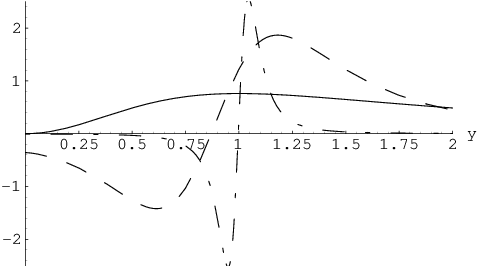
In Fig. 1 scaled plots of $Y_{\alpha}$ are shown. The function $X_{1}$ is the Cauchy probability density and $X_{1}^{(3)}$ is non-negative. For $\alpha\leq 1$ the function $X_{\alpha}$ is unimodular with a singularity at $y=0$ and therefore $X^{(3)}_{\alpha}$ is non-negative. For $\alpha>1$ the maximum of $X_{\alpha}$ is shifted to the right of $y=0$ and therefore the function $X^{(3)}_{\alpha}$ changes sign.

The parameter $\xi$ scales the spatial coordinates of the component waves $Y_{\alpha}$. The function $M_{\gamma}(\xi)$ represents the weights of various scalings of the solution. In Fig. 2 the function $M_{\gamma}(z)$ is plotted for $\gamma=1/2,1/3,2,3$. The shift of the maximum of the Wright function for $\gamma>1/2$ is noteworthy.

The functions $G^{(d)}_{(2/3,\alpha}$ for $d=1,3$ and $\alpha=1.5$ and $1.9$ are shown in Fig. 3 and Fig. 4. The values of $\beta$ are 1, and 1.2666.

We now assume that $\hat{Q}(\mathbf{k})$ is given by equation (2). The inverse Laplace transform of $\hat{\tilde{G}}(p,\mathbf{k})$ and $\hat{\tilde{H}}(p,\mathbf{k})$ is $E_{\beta}\left(\hat{Q}(\mathbf{k})\,t^{\beta}\right)$ and $E_{\beta,2}\left(\hat{Q}(\mathbf{k})\,t^{\beta}\right)$, respectively or, equivalently, $E_{\beta}\left(-k^{\alpha}\,F(\hat{\mathbf{k}})\,t^{\beta}\right)$ and $E_{\beta,2}\left(-k^{\alpha}\,F(\hat{\mathbf{k}})\,t^{\beta}\right)$, respectively, where $k:=|\mathbf{k}|$, $\hat{\mathbf{k}}:=k^{-1}\,\mathbf{k}$ and $F(\hat{\mathbf{k}})=-\hat{Q}(\hat{\mathbf{k}})$. The Mittag-Leffler function $E_{\lambda,\mu}(z)$ is defined in the appendix and $E_{\lambda}:=E_{\lambda,1}$.

We shall begin with the case $\beta=\alpha>1$.

The first fundamental solution can be obtained by inverting the Laplace and Fourier transform:

$$G(t,x)=\frac{1}{(2\uppi)^{3}}\int_{0}^{\infty}k^{2}\,\mathrm{d}k\int_{\mathcal{S}}\mathrm{d}_{2}\hat{\mathbf{k}}\,E_{\alpha}\left(-k^{\alpha}\,F(\hat{\mathbf{k}})\,t^{\alpha}\right)\,\mathrm{e}^{\mathrm{i}\mathbf{k}\cdot x}=\\ -\nabla^{2}\,\frac{1}{(2\uppi)^{3}\,t}\,\int_{\mathcal{S}}\mathrm{d}_{2}\hat{\mathbf{k}}\,F(\hat{\mathbf{k}})^{-1/\alpha}\int_{0}^{\infty}E_{\alpha}\left(-\kappa^{\alpha}\right)\,\mathrm{e}^{\mathrm{i}\kappa\,\left[(\hat{\mathbf{k}}\cdot\hat{x})\,r/F(\hat{\mathbf{k}})^{1/\alpha}\,t\right]}\,\mathrm{d}\kappa=:G^{(3)}_{1,\alpha}(t,x)$$

where $\hat{x}:=r^{-1}\,x$. The inverse Fourier transforms of $E_{\alpha}\left(-\kappa^{\alpha}\right)$ and $E_{\alpha,2}\left(-\kappa^{\alpha}\right)$ are $X_{\alpha}(y)$ and $Y_{\alpha}(y)$, respectively (Appendix E), hence

	$$\displaystyle G^{(3)}_{1,\alpha}(t,x)=-\frac{1}{(2\uppi)^{3}\,t}\int_{\mathcal{S}}\frac{\mathrm{d}_{2}\hat{\mathbf{k}}}{F(\hat{\mathbf{k}})^{1/\alpha}}\,\nabla^{2}\,X_{\alpha}\left(\hat{\mathbf{k}}\cdot\hat{x}\frac{r}{t\,F(\hat{\mathbf{k}})^{1/\alpha}}\right)$$		(47)
	$$\displaystyle H^{(3)}_{1,\alpha}(t,x)=-\frac{1}{(2\uppi)^{3}\,t}\int_{\mathcal{S}}\frac{\mathrm{d}_{2}\hat{\mathbf{k}}}{F(\hat{\mathbf{k}})^{1/\alpha}}\,\nabla^{2}\,Y_{\alpha}\left(\hat{\mathbf{k}}\cdot\hat{x}\frac{r}{t\,F(\hat{\mathbf{k}})^{1/\alpha}}\right)$$		(48)

The subscript ”1” refers to the value of $\gamma=\beta/\alpha$.

Choosing the spherical coordinates $(r,\vartheta,\varphi)$ in the $x$-space in such a way that $\hat{kk}$ corresponds to $\vartheta=0$ and $\hat{\mathbf{k}}\cdot\hat{x}=\cos(\vartheta)$, and substituting

$$\nabla^{2}=\frac{1}{r^{2}}\frac{\partial}{\partial r}\left(r^{2}\frac{\partial}{\partial r}\right)+\frac{1}{\sin(\vartheta)}\frac{\partial}{\partial\vartheta}\left(\sin(\vartheta)\frac{\partial}{\partial\vartheta}\right)$$

a rather complicated but fairly explicit expression is obtained.

We shall denote the functions $G(t,x)$ and $H(t,x)$ obtained above by $G^{\mu}_{1,\alpha}(t,x)$ and $H^{\mu}_{1,\alpha}(t,x)$.

For the case $\beta<\alpha$ we shall use the identity

$$E_{\beta}(-y)=\int_{0}^{\infty}M_{\gamma}(\xi)\,E_{\alpha}\left(-y\,\xi^{\alpha}\right)\,\mathrm{d}\xi$$

(49)

where $\gamma=\beta/\alpha$, see Appendix C. Hence, setting $t=1$ for simplicity,

$$E_{\beta}\left(-k^{\alpha}\,F(\hat{\mathbf{k}}\,t^{\beta})\right)=\int_{0}^{\infty}M_{\gamma}(\xi)\,E_{\alpha}\left(-\xi^{\alpha}\,k^{\alpha}\,F\left(\hat{\mathbf{k}}\,\left(t^{\gamma}\right)^{\alpha}\right)\right)\,\mathrm{d}\xi$$

Applying the inverse Fourier transformation we get the first fundamental solution $G^{\mu}_{\gamma,\alpha}$,

$$G^{\mu}_{\gamma,\alpha}(t,x)=\int_{0}^{\infty}M_{\gamma}(\xi)\,G^{\mu}_{1,\alpha}\left(t^{\gamma},x/\xi\right)\,\frac{\mathrm{d}\xi}{\xi}$$

(50)

or, equivalently

$$G^{\mu}_{\gamma,\alpha}(t,x)=\int_{0}^{\infty}M_{\gamma}(\xi)\,G^{\mu}_{1,\alpha}\left(1,y/\xi\right)\,\frac{\mathrm{d}\xi}{\xi}$$

(51)

where $y=x/t^{\gamma}$. Similarly the second fundamental solution is given by the Mellin convolution

$$H^{\mu}_{\gamma,\alpha}(t,x)=\int_{0}^{\infty}N_{\gamma}(\xi)\,G^{\mu}_{1,\alpha}\left(1,y/\xi\right)\,\frac{\mathrm{d}\xi}{\xi}$$

(52)

References

• Diethelm [2010] K. Diethelm. The Analysis of Fractional Differential Equations. Springer, Heidelberg, 2010.
• Gel’fand and Shilov [1964] I. M. Gel’fand and G. E. Shilov. Generalized Functions, volume I. Academic Press, New York, 1964.
• Gorenflo et al. [1999] R. Gorenflo, Yu. Luchko, and F. Mainardi. Analytical properties and applications of the Wright function. Fractional Calculus and Applied Analysis, 2:383–414, 1999.
• Gripenberg et al. [1990] G. Gripenberg, S. O. Londen, and O. J. Staffans. Volterra Integral and Functional Equations. Cambridge University Press, Cambridge, 1990.
• Hanyga [2002] A. Hanyga. Multi-dimensional solutions of space-time fractional diffusion equations. Proc. Roy. Soc. London A, 458:429–450, 2002.
• Hanyga and Seredyńska [2002] A. Hanyga and M. Seredyńska. Asymptotic wavefront expansions in hereditary media with singular memory kernels. Quart. Appl. Math., LX:213–244, 2002.
• Hanyga and Seredyńska [2007] A. Hanyga and M. Seredyńska. Relations between relaxation modulus and creep compliance in anisotropic linear viscoelasticity. J. of Elasticity, 88:41–61, 2007.
• Lu and Hanyga [2005] Jian-Fei Lu and A. Hanyga. Wave field simulation for heterogeneous porous media with a singular memory drag force. J. Comp. Phys., 208:651–674, 2005. doi: 10.1016/j.jcp.2005.03.008.
• Luchko [2008] Yu. Luchko. Algorithms for the evaluation of the Wright function for the real argument values. Fractional Calculus and Applied Analysis, 11, 2008.
• Luchko et al. [2010] Yu. Luchko, J. J. Trujillo, and M. P. Velasco. The Wright function and its numerical evaluation. International J. of Pure and Applied Mathematics, 64:567–575, 2010.
• Mainardi [2011] F. Mainardi. On the distinguished role of the Mittag-Leffler and Wright functions in fractional calculus. In Special Functions in the 21st Century: Theory and Applications, Washington DC, USA, 6–8 April, 2011.
• Mainardi et al. [2001] F. Mainardi, Yu. Luchko, and G. Pagnini. The fundamental solution of the space-time fractional diffusion equation. Fractional Calculus and Applications, 4:153–192, 2001.
• Mainardi et al. [2010] F. Mainardi, A. Mura, and G. Pagnini. The MM-Wright function in time-fractional diffusion processes: A tutorial survey. Int. J. Differential Equations, 2010:ID 104505, 2010.
• Özarslan and Mareci [2003] E. Özarslan and T. Mareci. Generalized Diffusion Tensor Imaging and analytical relationships between Diffusion Tensor Imaging and High Angular Resolution Diffusion Imaging. Magnetic Resonance in Med., 50:(55–965, 2003.
• Podlubny [1998] I. Podlubny. Fractional Differential Equations. Academic Press, San Diego, 1998.
• Samko et al. [1993] S. G. Samko, A. A. Kilbas, and O. I. Marichev. Fractional Integrals and Derivatives, Theory and Applications. Gordon and Breach, Amsterdam, 1993.
• Yuan and Agrawal [1998] L. Yuan and O. P. Agrawal. A numerical scheme for dynamic systems containing fractional derivatives. In Proceedings of DETC’98, ASME Design Engineering Technical Conferences, September 13–16, 1998, Atlanta, GA, 1998.
Appendix A Some definitions
A function ff on the open positive real half-line ]0,∞[]0,\infty[ is said to be completely monotone (CM) if it is infinitely differentiable and (−1)n​Dn​f​(t)≥0(-1)^{n}\,\mathrm{D}^{n}\,f(t)\geq 0 for every non-negative integer nn and t>0t>0.
A CM function can have a singularity at 0. A CM function is locally integrable (LICM) if it its integral over the segment [0,1][0,1] is finite.
A measurable real function ff on [0,∞[[0,\infty[ is said to be causally positive definite (CPD) if
∫−∞∞∫0∞f⁡(y)​φ​(x−y)​φ​(x)≥0\int_{-\infty}^{\infty}\int_{0}^{\infty}f(y)\,\varphi(x-y)\,\varphi(x)\geq 0
for every compactly supported real test function φ\varphi.
By a theorem in Gripenberg et al. [1990] every LICM function is CPD. Gripenberg’s extension of Bochner’s theorem asserts that every continuous CPD function is equal for x≥0x\geq 0 to the Fourier transform of a finite positive Radon measure. For our purposes a the restriction to bounded functions is unwelcome. The Bochner-Schwartz theorem is an extension of Bochner’s theorem to positive definite tempered distributions:
Theorem A.1
A causal positive definite tempered distribution ff is the Fourier transform of a positive tempered Radon measure:
f(x)=∫−∞∞e−i𝐤⋅xμ(d𝐤),x>0f(x)=\int_{-\infty}^{\infty}\mathrm{e}^{-\mathrm{i}\mathbf{k}\cdot x}\,\mu(\mathrm{d}\mathbf{k}),\qquad x>0
where μ\mu is a tempered Radon measure (i.e. a non-negative tempered distribution). This theorem captures functions with singularities typical of Gelfand’s homogeneous distributions.
Appendix B Wright functions
The Wright function depend on two parameters. They are defined in terms of power series expansion
Wλ,μ​(z):=∑n=0∞znn!​Γ​(n​λ+μ),λ>−1,μ∈ℂW_{\lambda,\mu}(z):=\sum_{n=0}^{\infty}\frac{z^{n}}{n!\,\Gamma(n\lambda+\mu)},\qquad\lambda>-1,\;\mu\in\mathbb{C}
They also have an integral representation
Wλ,μ​(z)=12​π​i​∫ℋep−z​p−λ​d​ppμ,λ>−1,μ∈ℂW_{\lambda,\mu}(z)=\frac{1}{2\uppi\mathrm{i}}\int_{\mathcal{H}}\mathrm{e}^{p-z\,p^{-\lambda}}\frac{\mathrm{d}p}{p^{\mu}},\qquad\lambda>-1,\;\mu\in\mathbb{C}
where ℋ\mathcal{H} denotes the Hankel contour encircling the cut along the negative real axis, as shown in Fig. 5.
The Wright functions MγM_{\gamma} and NγN_{\gamma} are special cases of the Wright function
Mγ​(z)=W−γ,1−γ​(−z)\displaystyle M_{\gamma}(z)=W_{-\gamma,1-\gamma}(-z) (53)
Nγ​(z)=W−γ,2−γ​(−z)\displaystyle N_{\gamma}(z)=W_{-\gamma,2-\gamma}(-z) (54)
The best review paper on the Wright function and MγM_{\gamma} is Mainardi [2011]. The function NγN_{\gamma} has not been studied before. Their series expansions are
Mγ​(z)=∑n=0∞(−z)nn!​Γ​(1−γ⁡(n+1)CLOSE=1π​∑n=1∞(−z)n−1(n−1)!​Γ​(n​γ)​sin⁡(n​π​γ)\displaystyle M_{\gamma}(z)=\sum_{n=0}^{\infty}\frac{(-z)^{n}}{n!\,\Gamma(1-\gamma\,(n+1)}=\frac{1}{\uppi}\sum_{n=1}^{\infty}\frac{(-z)^{n-1}}{(n-1)!}\Gamma(n\,\gamma)\,\sin(n\,\uppi\gamma) (55)
Nγ​(z)=∑n=0∞(−z)nn!​Γ​(2−γ⁡(n+1)CLOSE\displaystyle N_{\gamma}(z)=\sum_{n=0}^{\infty}\frac{(-z)^{n}}{n!\,\Gamma(2-\gamma\,(n+1)} (56)
These functions also have the integral representations
Mγ​(z)=12​π​i​∫ℋξγ−1​eξ−z​ξγ​𝑑ξ\displaystyle M_{\gamma}(z)=\frac{1}{2\uppi\mathrm{i}}\int_{\mathcal{H}}\xi^{\gamma-1}\,\mathrm{e}^{\xi-z\,\xi^{\gamma}}\,\mathrm{d}\xi (57)
Nγ​(z)=12​π​i​∫ℋξγ−2​eξ−z​ξγ​𝑑ξ\displaystyle N_{\gamma}(z)=\frac{1}{2\uppi\mathrm{i}}\int_{\mathcal{H}}\xi^{\gamma-2}\,\mathrm{e}^{\xi-z\,\xi^{\gamma}}\,\mathrm{d}\xi (58)
Refer to caption
Figure 5: The Hankel contour ℋ\mathcal{H}.
Numerical methods of evaluating the Wright functions can be found in Luchko et al. [2010] and Luchko [2008].
The Mellin transform of Mγ​(z)M_{\gamma}(z) is Γ⁡(1−s)/Γ⁡(1−γ​s)\Gamma(1-s)/\Gamma(1-\gamma s) and
Mγ​(z)=12​π​i​∫−ε−i​∞−ε+i​∞Γ⁡(1−s)Γ⁡(1−γ​s)​z−s​𝑑sfor z>0, 0<γ<1, 0<ε<1M_{\gamma}(z)=\frac{1}{2\uppi\mathrm{i}}\int_{-\varepsilon-\mathrm{i}\infty}^{-\varepsilon+\mathrm{i}\infty}\frac{\Gamma(1-s)}{\Gamma(1-\gamma s)}\,z^{-s}\,\mathrm{d}s\quad\text{for $z>0$, $0<\gamma<1$, $0<\varepsilon<1$} (59)
As a rough check note that for z>1z>1 the Bromwich contour can be closed in the right ss half-plane. The contribution of the poles of Γ⁡(1−s)\Gamma(1-s) at s=n+1s=n+1, n=0,1,2,…n=0,1,2,\ldots is
∑n=0∞(−1)n​znn!​Γ​(1−(n+1)​γ)=Mγ​(z)\sum_{n=0}^{\infty}(-1)^{n}\frac{z^{n}}{n!\,\Gamma(1-(n+1)\,\gamma)}=M_{\gamma}(z)
Similarly, the Mellin transform of Nγ​(z)N_{\gamma}(z) is Γ⁡(1−s)/Γ⁡(2−γ​s)\Gamma(1-s)/\Gamma(2-\gamma s).
Appendix C Proof of identity (49) and related results.
Lemma C.1
Eβ​(−z)=12​π​i​∫ℬΓ⁡(s)​Γ​(1−s)Γ⁡(1−β​s)​z−s​𝑑s\displaystyle E_{\beta}(-z)=\frac{1}{2\uppi\mathrm{i}}\int_{\mathcal{B}}\frac{\Gamma(s)\,\Gamma(1-s)}{\Gamma(1-\beta s)}z^{-s}\,\mathrm{d}s (60)
Eβ,2​(−z)=12​π​i​∫ℬΓ⁡(s)​Γ​(1−s)Γ⁡(2−β​s)​z−s​𝑑s\displaystyle E_{\beta,2}(-z)=\frac{1}{2\uppi\mathrm{i}}\int_{\mathcal{B}}\frac{\Gamma(s)\,\Gamma(1-s)}{\Gamma(2-\beta s)}z^{-s}\,\mathrm{d}s (61)
Proof. Since Γ⁡(s)​Γ​(1−s)=π/sin⁡(π​s)\Gamma(s)\,\Gamma(1-s)=\uppi/\sin(\uppi s), the integrand on the right-hand side of equation (60) has poles at s=n=0,±1,±2,…s=n=0,\pm 1,\pm 2,\ldots. Stirling’s formula
Γ(z)=2​πz−1/2(z/e)z(1+O[1/z])for |arg⁡(z)|<π−ε, ε>0\Gamma(z)=\sqrt{2\uppi}\,z^{-1/2}\,(z/\mathrm{e})^{z}\,(1+\mathrm{O}[1/z])\qquad\text{for $|\arg(z)|<\uppi-\varepsilon$, $\varepsilon>0$}
implies that for Re​s→−∞\mathrm{Re}s\rightarrow-\infty
z−s/Γ(1−βs)∼s→∞(−βs)1/2/2​πexp((βs−1)[ln(1−βs)−1]−sln(z))z^{-s}/\Gamma(1-\beta\,s)\sim_{s\rightarrow\infty}(-\beta s)^{1/2}/\sqrt{2\uppi}\,\exp\left((\beta s-1)\,[\ln(1-\beta s)-1]-s\,\ln(z)\right)
The first term in the exponent dominates and therefore the integrand vanishes for Re​s→−∞\mathrm{Re}s\rightarrow-\infty faster than 1/|s|1/|s|. Hence the Bromwich contour can be closed by a half-circle at infinity in the left half of the complex ss-plane without changing the value of the integral. The only singularities inside the closed contour thus obtained are the poles at s=0,−1,−2,s=0,-1,-2,. Their residues are (−z)n/Γ⁡(1+β​n)(-z)^{n}/\Gamma(1+\beta n). Hence the right-hand side of equation (60) is equal to
∑n=0∞(−z)nΓ⁡(1+n​β)≡Eβ​(−z)\sum_{n=0}^{\infty}\frac{(-z)^{n}}{\Gamma(1+n\,\beta)}\equiv E_{\beta}(-z)
The proof of equation (61) is analogous. □\Box
The integrands on the right hand side of (60) and (61) are thus Mellin transforms of the left-hand sides:
∫0∞Eβ​(−x)​xs−1​𝑑s=Γ⁡(s)​Γ​(1−s)Γ⁡(1−β​s)\displaystyle\int_{0}^{\infty}E_{\beta}(-x)\,x^{s-1}\,\mathrm{d}s=\frac{\Gamma(s)\,\Gamma(1-s)}{\Gamma(1-\beta s)} (62)
∫0∞Eβ,2​(−x)​xs−1​𝑑s=Γ⁡(s)​Γ​(1−s)Γ⁡(2−β​s)\displaystyle\int_{0}^{\infty}E_{\beta,2}(-x)\,x^{s-1}\,\mathrm{d}s=\frac{\Gamma(s)\,\Gamma(1-s)}{\Gamma(2-\beta s)} (63)
Lemma C.2
Mγ​(y)=12​π​i​∫ℬΓ⁡(s)Γ⁡(1+γ⁡(s−1))​y−s​𝑑s0<γ<1\displaystyle M_{\gamma}(y)=\frac{1}{2\uppi\mathrm{i}}\int_{\mathcal{B}}\frac{\Gamma(s)}{\Gamma(1+\gamma(s-1))}y^{-s}\,\mathrm{d}s\qquad 0<\gamma<1 (64)
Nγ​(y)=12​π​i​∫ℬΓ⁡(s)Γ⁡(2+γ⁡(s−1))​y−s​𝑑s0<γ<1\displaystyle N_{\gamma}(y)=\frac{1}{2\uppi\mathrm{i}}\int_{\mathcal{B}}\frac{\Gamma(s)}{\Gamma(2+\gamma(s-1))}y^{-s}\,\mathrm{d}s\qquad 0<\gamma<1 (65)
Proof. The proof is similar to the proof of Lemma C.1. The residues of Γ⁡(s)\Gamma(s) at s=−ns=-n, n=0,1,…n=0,1,\ldots. are (−1)n/n!(-1)^{n}/n!, hence the integral on the right-hand side of (64) is equal to
∑n=0∞znn!​Γ​(1−γ⁡(n+1)),\sum_{n=0}^{\infty}\frac{z^{n}}{n!\,\Gamma(1-\gamma(n+1))},
which is equal to the function on the left-hand side.
The other equation is proved in the same way. □\Box
We are now ready to prove the following important relations
Eβ​(−κα)=∫0∞Mγ​(ξ)​Eα​(−(κ​ξ)α)​𝑑ξ\displaystyle E_{\beta}\left(-\kappa^{\alpha}\right)=\int_{0}^{\infty}M_{\gamma}(\xi)\,E_{\alpha}\left(-(\kappa\xi)^{\alpha}\right)\,\mathrm{d}\xi (66)
Eβ,2​(−κα)=∫0∞Nγ​(ξ)​Eα​(−(κ​ξ)α)​𝑑ξ\displaystyle E_{\beta,2}\left(-\kappa^{\alpha}\right)=\int_{0}^{\infty}N_{\gamma}(\xi)\,E_{\alpha}\left(-(\kappa\xi)^{\alpha}\right)\,\mathrm{d}\xi (67)
where 0<γ=β/α<10<\gamma=\beta/\alpha<1.
Equation (60) implies that
Eβ​(−κα)=12​π​i​α​∫ℬΓ⁡(s/α)​Γ​(1−s/α)Γ⁡(1−γ​s)​κ−s​𝑑sE_{\beta}(-\kappa^{\alpha})=\frac{1}{2\uppi\mathrm{i}\alpha}\int_{\mathcal{B}}\frac{\Gamma(s/\alpha)\,\Gamma(1-s/\alpha)}{\Gamma(1-\gamma s)}\kappa^{-s}\,\mathrm{d}s (68)
while equation (64) implies that
1ξ​Mγ​(1/ξ)=12​π​i​∫ℬΓ⁡(1−s)Γ⁡(1−γ​s)​ξ−s​𝑑s\frac{1}{\xi}M_{\gamma}(1/\xi)=\frac{1}{2\uppi\mathrm{i}}\int_{\mathcal{B}}\frac{\Gamma(1-s)}{\Gamma(1-\gamma s)}\xi^{-s}\,\mathrm{d}s (69)
We now recall that the Mellin transform of the Mellin convolution
∫0∞f⁡(ξ)​g​(x/ξ)​d​ξξ\int_{0}^{\infty}f(\xi)\,g(x/\xi)\frac{\mathrm{d}\xi}{\xi}
of two functions ff and gg is equal to the product of the Mellin transforms of ff and gg. Hence
Eβ​(−κα)=∫0∞1ξ​Mγ​(1/ξ)​Eα​(−(κ/ξ)α)​d​ξξ=∫0∞Mγ​(ζ)​Eα​(−(κ​ζ)α)​𝑑ζE_{\beta}\left(-\kappa^{\alpha}\right)=\int_{0}^{\infty}\frac{1}{\xi}M_{\gamma}(1/\xi)\,E_{\alpha}\left(-(\kappa/\xi)^{\alpha}\right)\frac{\mathrm{d}\xi}{\xi}=\int_{0}^{\infty}M_{\gamma}(\zeta)\,E_{\alpha}\left(-(\kappa\zeta)^{\alpha}\right)\,\mathrm{d}\zeta
This proves equation (66). Equation (67) is proved in a similar way.
The identities (66) and (67) have an important corollary. Applying the inverse Fourier transform to both sides of either identity and noting (36) we obtain the relations
Gβ,α​(1,x)=∫0∞Mγ​(ξ)​Gα,α​(1,x/ξ)​d​ξξ\displaystyle G_{\beta,\alpha}(1,x)=\int_{0}^{\infty}M_{\gamma}(\xi)\,G_{\alpha,\alpha}(1,x/\xi)\,\frac{\mathrm{d}\xi}{\xi} (70)
Hβ,α​(1,x)=∫0∞Nγ​(ξ)​Gα,α​(1,x/ξ)​d​ξξ\displaystyle H_{\beta,\alpha}(1,x)=\int_{0}^{\infty}N_{\gamma}(\xi)\,G_{\alpha,\alpha}(1,x/\xi)\,\frac{\mathrm{d}\xi}{\xi} (71)
Appendix D The functions M2/3​(z)M_{2/3}(z) and N2/3​(z)N_{2/3}(z).
A method for numerical computation of the Wright function can be found in Luchko et al. [2010], Luchko [2008].
Explicit representations of MγM_{\gamma} exist for γ=1/3,1/2\gamma=1/3,1/2 and 2/32/3. The first two can be found in Mainardi [2011]. Since we are interested in wave equations, only γ>1/2\gamma>1/2 is of interest to us.
The function M2/3​(z)M_{2/3}(z) can be expressed in terms of the Airy function using the results obtained in Hanyga and Seredyńska [2002] for the function
f1(3)​(t,λ1,λ2)=−∂∂λ2​f2(3)​(t,λ1,λ2)f_{1}^{(3)}(t,\lambda_{1},\lambda_{2})=-\frac{\partial}{\partial\lambda_{2}}f_{2}^{(3)}(t,\lambda_{1},\lambda_{2}) (72)
where
f2(3)(t,λ1,λ2):=12​π​i∫ℬs−2/3es​te−λ1​s2/3−λ2​s1/3dsf_{2}^{(3)}(t,\lambda_{1},\lambda_{2}):=\frac{1}{2\uppi\mathrm{i}}\int_{\mathcal{B}}s^{-2/3}\,\mathrm{e}^{st}\,\mathrm{e}^{-\lambda_{1}\,s^{2/3}-\lambda_{2}s^{1/3}}\,\mathrm{d}s (73)
and ℬ\mathcal{B} denotes the Bromwich contour. The function f2(3)f^{(3)}_{2} can be expressed in terms of the Airy function as follows:
f2(3)(t,λ1,λ2)=32/3t1/3Ai((3t)−1/3(λ2+λ1;23​t))exp(−λ13​t(λ2+2λ1;29​t))f_{2}^{(3)}(t,\lambda_{1},\lambda_{2})=\frac{3^{2/3}}{t^{1/3}}\mathrm{Ai}\left((3t)^{-1/3}\,\left(\lambda_{2}+\frac{\lambda_{1}^{;2}}{3t}\right)\right)\,\exp\left(-\frac{\lambda_{1}}{3t}\left(\lambda_{2}+\frac{2\lambda_{1}^{;2}}{9t}\right)\right) (74)
On the other hand straightforward transformations of the integration variable in (73) yield the relation
M2/3(z)=f1(3)(z−3/2,1,0)/zM_{2/3}(z)=f_{1}^{(3)}\left(z^{-3/2},1,0\right)/z (75)
It is to be noted that the Hankel contour in (57) can be replaced by the Bromwich contour.
Equation (75) can be worked out in terms of the Airy function
M2/3(z)=[3−1/3zAi(z2/34/3)−31/3Ai′(z2/34/3)]e−2z3/27M_{2/3}(z)=\left[3^{-1/3}\,z\,\mathrm{Ai}\left(z^{2}/3^{4/3}\right)-3^{1/3}\mathrm{Ai}^{\prime}\left(z^{2}/3^{4/3}\right)\right]\,\mathrm{e}^{-2z^{3}/27} (76)
or in terms of the modified Bessel function of the second kind
M2/3(z)=z233/2​π[K1/3(227z3)+K2/3(227z3)]e−2z3/27M_{2/3}(z)=\frac{z^{2}}{3^{3/2}\,\uppi}\left[K_{1/3}\left(\frac{2}{27}z^{3}\right)+K_{2/3}\left(\frac{2}{27}z^{3}\right)\right]\,\mathrm{e}^{-2z^{3}/27} (77)
A simple expression for the function U1(2/3,α)​(y)U_{1}^{(2/3,\alpha)}(y) can be derived from equation (77):
U1(2/3,α)​(y)=32​π​∫0∞Z⁡(ζ)​Xα​(21/3​y/(3​ζ1/3))​𝑑ζU_{1}^{(2/3,\alpha)}(y)=\frac{\sqrt{3}}{2\uppi}\int_{0}^{\infty}Z(\zeta)\,X_{\alpha}\left(2^{1/3}\,y/\left(3\,\zeta^{1/3}\right)\right)\,\mathrm{d}\zeta (78)
Z⁡(ζ):=(K1/3​(ζ)+K2/3​(ζ))​e−ζZ(\zeta):=\left(K_{1/3}(\zeta)+K_{2/3}(\zeta)\right)\,\mathrm{e}^{-\zeta} (79)
In order to express N2/3N_{2/3} in terms of the Airy functions, we define a new function
F(t,λ1,λ2):=∫0λ1f2(3)(t,ξ,λ2)dξ≡12​π​i∫ℬs−4/3es​te−λ1​s2/3−λ2​s1/3dsF(t,\lambda_{1},\lambda_{2}):=\int_{0}^{\lambda_{1}}f_{2}^{(3)}(t,\xi,\lambda_{2})\,\mathrm{d}\xi\equiv\frac{1}{2\uppi\mathrm{i}}\int_{\mathcal{B}}s^{-4/3}\,\mathrm{e}^{st}\,\mathrm{e}^{-\lambda_{1}\,s^{2/3}-\lambda_{2}s^{1/3}}\,\mathrm{d}s
In terms of this function
N3/2(z)=z1/2∫01F(z−3/2,ξ,0)dξN_{3/2}(z)=z^{1/2}\int_{0}^{1}F\left(z^{-3/2},\xi,0\right)\,\mathrm{d}\xi
Substituting (74) the following alternative formula is derived
N2/3(z)=32/3z−1∫0zζ1/2Ai(3−4/3ζ2)exp(−227ζ3)dζN_{2/3}(z)=3^{2/3}\,z^{-1}\int_{0}^{z}\zeta^{1/2}\,\mathrm{Ai}\left(3^{-4/3}\,\zeta^{2}\right)\,\exp\left(-\frac{2}{27}\,\zeta^{3}\right)\,\mathrm{d}\zeta (80)
N2/3N_{2/3} can be further simplified by substituting
Ai(x)=1π3−1/2x1/2K1/3(23x3/2)\mathrm{Ai}(x)=\frac{1}{\uppi}3^{-1/2}\,x^{1/2}\,K_{1/3}\left(\frac{2}{3}x^{3/2}\right)
which yields the formula
N2/3(z)=325/6​π​z∫02​z3/27y−1/6K1/3(y)e−ydyN_{2/3}(z)=\frac{3}{2^{5/6}\,\uppi z}\int_{0}^{2z^{3}/27}y^{-1/6}\,K_{1/3}(y)\,\mathrm{e}^{-y}\,\mathrm{d}y (81)
or
N2/3(z)=z1/2π​3[Γ(1/3)2F2(1/6,1/2;1/3,1/2;−4z3/27)−17Γ(2/3)z22F2(5/6,7/6;5/3,13/3;−4z3/27)]N_{2/3}(z)=\frac{z^{1/2}}{\uppi\sqrt{3}}[\Gamma(1/3)\;_{2}F_{2}\left(1/6,1/2;1/3,1/2;-4z^{3}/27\right)\\ -\frac{1}{7}\Gamma(2/3)\,z^{2}\,_{2}F_{2}\left(5/6,7/6;5/3,13/3;-4z^{3}/27\right)] (82)
The functions M2/3M_{2/3} and N2/3N_{2/3} are shown in Fig. 6.
Figure 6: Plots of M2/3​(z)M_{2/3}(z) (solid line) and N2/3​(z)N_{2/3}(z) (dashed line).
Appendix E The inverse Fourier transform of Eα​(−|k|α)E_{\alpha}\left(-|k|^{\alpha}\right).
Applying the inverse Fourier transformation to both sides of the identity
Eα​(−|k|α)=∑n=0∞(−1)n​|k|α​nΓ⁡(1+α​n)E_{\alpha}\left(-|k|^{\alpha}\right)=\sum_{n=0}^{\infty}(-1)^{n}\,\frac{|k|^{\alpha n}}{\Gamma(1+\alpha n)}
and recalling the Fourier transform of |k|α|k|^{\alpha} is −2​sin⁡(n​α​π/2)​Γ​(1+α​n)​|x|−α−1-2\sin(n\alpha\uppi/2)\,\Gamma(1+\alpha n)\,|x|^{-\alpha-1} Gel’fand and Shilov [1964] we have
12​π∫−∞∞ei​k​xEα(−|k|α)dk=−2Im∑n=0∞(−1)n|x|−α​n−1(ei​α​π/2)n=−2|x|​Im​11+|x|−α​ei​π​α/2\frac{1}{2\uppi}\int_{-\infty}^{\infty}\mathrm{e}^{\mathrm{i}kx}\,E_{\alpha}\left(-|k|^{\alpha}\right)\,\mathrm{d}k=-2\mathrm{Im}\sum_{n=0}^{\infty}(-1)^{n}\,|x|^{-\alpha n-1}\,\left(\mathrm{e}^{\mathrm{i}\alpha\uppi/2}\right)^{n}=\\ -\frac{2}{|x|}\mathrm{Im}\frac{1}{1+|x|^{-\alpha}\,\mathrm{e}^{\mathrm{i}\uppi\alpha/2}}
so that
Gα,α​(1,x)≡Xα​(x)=12​π​i​∫−∞∞ei​k​x​Eα,α​(−|k|α)​dk=sin⁡(π​α/2)π​|x|α−1|x|2​α+2​|x|α​cos⁡(π​α/2)+1G_{\alpha,\alpha}(1,x)\equiv X_{\alpha}(x)=\frac{1}{2\uppi\mathrm{i}}\int_{-\infty}^{\infty}\mathrm{e}^{\mathrm{i}kx}\,E_{\alpha,\alpha}\left(-|k|^{\alpha}\right)\,\mathrm{d}k=\\ \frac{\sin(\uppi\alpha/2)}{\uppi}\frac{|x|^{\alpha-1}}{|x|^{2\alpha}+2|x|^{\alpha}\,\cos(\uppi\alpha/2)+1} (83)
Mainardi et al. [2001].
The second Green’s function Hα,αH_{\alpha,\alpha} is somewhat more difficult to calculate
Hα,α​(1,x)≡Yα​(x)=12​π​∫−∞∞ei​k​x​Eα,2​(−|k|α)​𝑑k=:F⁡(|x|)H_{\alpha,\alpha}(1,x)\equiv Y_{\alpha}(x)=\frac{1}{2\uppi}\int_{-\infty}^{\infty}\mathrm{e}^{\mathrm{i}kx}\,E_{\alpha,2}\left(-|k|^{\alpha}\right)\,\mathrm{d}k=:F(|x|)
But
Eα,2​(−κα)=∑n=0∞(−1)n​κα​nΓ⁡(2+α​n)E_{\alpha,2}\left(-\kappa^{\alpha}\right)=\sum_{n=0}^{\infty}(-1)^{n}\,\frac{\kappa^{\alpha n}}{\Gamma(2+\alpha n)}
Hence
F′(y)=−2y2Im∑n=0∞(−1)n(ei​α​n​π/2y)−α​n=2​sin⁡(α​π/2)​yα−2y2​α+2​yα​cos⁡(α​π/2)+1F^{\prime}(y)=-\frac{2}{y^{2}}\mathrm{Im}\sum_{n=0}^{\infty}(-1)^{n}\,\left(\mathrm{e}^{\mathrm{i}\alpha n\uppi/2}\,y\right)^{-\alpha n}=\\ 2\sin(\alpha\uppi/2)\,\frac{y^{\alpha-2}}{y^{2\alpha}+2y^{\alpha}\,\cos(\alpha\uppi/2)+1}
and F⁡(y)F(y) vanishes at infinity. Hence
F(y)=−2sin(απ/2)∫y∞zα−2z2​α+2​zα​cos⁡(α​π/2)+1dzF(y)=-2\sin(\alpha\uppi/2)\int_{y}^{\infty}\frac{z^{\alpha-2}}{z^{2\alpha}+2z^{\alpha}\,\cos(\alpha\uppi/2)+1}\mathrm{d}z (84)
Unlike Gα,αG_{\alpha,\alpha}, the function Hα,αH_{\alpha,\alpha} is not an algebraic function. For α=1/2\alpha=1/2 it can be expressed in terms of the logarithm.
Combining equations (83), (84), (70), (71) and (38) we get fairly explicit integral representations of the fundamental solutions of the Cauchy problem in one and three dimensions.