跳到论文正文
W Papers独立论文阅读器 arXiv:1111.1524 论文正文 计算阅读时间 · 0%
引用这篇论文根据当前论文元数据生成,正式投稿前建议核对。


License: arXiv.org perpetual non-exclusive license
arXiv:1111.1524v1 [math.NA] 07 Nov 2011

Multiscale Finite Element approach for ”weakly” random problems and related issues

Claude Le Bris    Frédéric Legoll    Florian Thomines Affiliation: École Nationale des Ponts et Chaussées, 6 et 8 avenue Blaise Pascal, 77455 Marne-La-Vallée Cedex 2 Affiliation: and INRIA Rocquencourt, MICMAC team-project, Domaine de Voluceau, B.P. 105, Affiliation: 78153 Le Chesnay Cedex, France Affiliation: lebris@cermics.enpc.fr, {legoll,thominef}@lami.enpc.fr
August 24, 2026
Abstract

We address multiscale elliptic problems with random coefficients that are a perturbation of multiscale deterministic problems. Our approach consists in taking benefit of the perturbative context to suitably modify the classical Finite Element basis into a deterministic multiscale Finite Element basis. The latter essentially shares the same approximation properties as a multiscale Finite Element basis directly generated on the random problem. The specific reference method that we use is the Multiscale Finite Element Method. Using numerical experiments, we demonstrate the efficiency of our approach and the computational speed-up with respect to a more standard approach. We provide a complete analysis of the approach, extending that available for the deterministic setting.

1 Overview of our approach and results

The Multiscale Finite Element Method (henceforth abbreviated as MsFEM) is a popular numerical approach for multiscale problems (see [37, 38, 30, 32, 31, 3, 39, 20, 18, 11]). It consists in a Galerkin approximation of the original problem over a finite dimensional space generated by basis functions that are specifically adapted to the problem under consideration.

This approach is popular for a twofold reason. First, its use is not restricted to multiscale problems that converge to a homogenized problem in the limit of vanishing ratio between the small scale and the macroscopic scale. It may be applied to much more general situations. Second, when the problem does converge to a homogenization problem, the MsFEM approach is meant to approximate the solution of the problem with the small scale ε\varepsilon at its actual small value and not ”only” in the asymptotic regime ε→0\varepsilon\to 0, which is the regime addressed by homogenization theory.

To fix the ideas, consider the problem of finding uεu^{\varepsilon} solving

−div[Aε∇uε]=fin 𝒟,uε=0on ∂𝒟,-\mbox{div}\left[A^{\varepsilon}\nabla u^{\varepsilon}\right]=f\ \ \mbox{in $\mathcal{D}$},\quad u^{\varepsilon}=0\ \ \mbox{on $\partial\mathcal{D}$}, (1)

on a bounded domain 𝒟⊂ℝd\mathcal{D}\subset\mathbb{R}^{d}, with f∈L2​(𝒟)f\in L^{2}(\mathcal{D}), and where AεA^{\varepsilon} is a uniformly bounded, coercive matrix that varies at scale ε\varepsilon. A standard Finite Element Method (FEM) would require a space discretization of the domain at the scale ε\varepsilon in order to capture the oscillations of uεu^{\varepsilon} at scale ε\varepsilon. This is prohibitively expensive. The MsFEM aims at accurately approximating uεu^{\varepsilon} using a limited number of degrees of freedom. It does not require the matrix AεA^{\varepsilon} to be periodic (namely Aε​(x)=Ap​e​r​(x/ε)A^{\varepsilon}(x)=A_{per}(x/\varepsilon) for a fixed periodic matrix Ap​e​rA_{per}) or stationary.

We now briefly describe the approach and present the aim of this article. Starting from a coarse mesh 𝒯h{\cal T}_{h} with a standard (say ℙ1\mathbb{P}_{1}) Finite Element basis set of functions {ϕi0}i=1L\left\{\phi_{i}^{0}\right\}_{i=1}^{L}, generating the associated space

𝒱h:=span​(ϕi0,i=1,⋯,L),{\cal V}_{h}:=\text{span}(\phi_{i}^{0},i=1,\cdots,L),

we first numerically build the MsFEM basis functions ϕiε\phi_{i}^{\varepsilon}. Several definitions of these basis functions have been proposed in the literature (yielding different numerical methods), and we detail this in the sequel (see e.g. (10)-(11)-(12)). For the moment, it is sufficient to know that, to each ϕi0\phi_{i}^{0}, which varies at the macroscopic scale, is associated a function ϕiε\phi_{i}^{\varepsilon}, with variations at the scale ε\varepsilon. In practice, ϕiε\phi_{i}^{\varepsilon} is numerically computed (in fact, pre-computed), using the specificities of the problem addressed. These highly oscillatory functions ϕiε\phi_{i}^{\varepsilon} generate the finite dimensional space

𝒲h:=span​(ϕiε,i=1,⋯,L).{\cal W}_{h}:=\text{span}(\phi_{i}^{\varepsilon},i=1,\cdots,L).

Note that 𝒲h{\cal W}_{h} and 𝒱h{\cal V}_{h} share the same dimension.

We next define the MsFEM solution uMu_{M} using a Galerkin approximation of (1) on 𝒲h{\cal W}_{h}, instead of 𝒱h{\cal V}_{h}. Again, details will be given below. The MsFEM solution uMu_{M} provided by the approach reads

uM​(x)=∑i=1L(UM)i​ϕiε​(x),u_{M}(x)=\sum\limits_{i=1}^{L}(U_{M})_{i}\ \phi_{i}^{\varepsilon}(x),

for some coefficients {(UM)i}i=1L\left\{(U_{M})_{i}\right\}_{i=1}^{L}. Of course, these coefficients depend on ε\varepsilon, but this dependency is kept implicit in the sequel.

We now turn our attention to the stochastic problem

−div[Aε(⋅,ω)∇uε(⋅,ω)]=fin 𝒟,uε(⋅,ω)=0on ∂𝒟,-\mbox{div}\left[A^{\varepsilon}(\cdot,\omega)\nabla u^{\varepsilon}(\cdot,\omega)\right]=f\ \ \mbox{in $\mathcal{D}$},\quad u^{\varepsilon}(\cdot,\omega)=0\ \ \mbox{on $\partial\mathcal{D}$}, (2)

and a typical quantity of interest 𝔼​[uε​(x,⋅)]\mathbb{E}\left[u^{\varepsilon}(x,\cdot)\right], which is traditionally approximated using a Monte Carlo method. Introducing a set of ℳ{\cal M} realizations of the stochastic matrix {Aε,m}1≤m≤ℳ\left\{A^{\varepsilon,m}\right\}_{1\leq m\leq{\cal M}}, a direct, naïve application of the MsFEM paradigm would consist in first computing for each realization mm the stochastic MsFEM basis functions ϕiε,m​(x,ω)\phi_{i}^{\varepsilon,m}(x,\omega), next performing a Galerkin approximation of (2) using this MsFEM basis set to compute {uMm​(x,ω)}1≤m≤ℳ\left\{u_{M}^{m}(x,\omega)\right\}_{1\leq m\leq{\cal M}}, and eventually approximating 𝔼​[uε​(x,⋅)]\mathbb{E}\left[u^{\varepsilon}(x,\cdot)\right] by

𝔼⁡[uε​(x,⋅)]≈1ℳ​∑m=1ℳuMm​(x,ω).\mathbb{E}\left[u^{\varepsilon}(x,\cdot)\right]\approx\frac{1}{\cal M}\sum_{m=1}^{\cal M}u_{M}^{m}(x,\omega).

Such an approach is unpractical because of the prohibitively expensive computational load.

To reduce the computational cost and make the MsFEM approach practical in such a stochastic context, a natural idea we investigate in this article is to consider a less generic setting, for which a dedicated, more computationally affordable approach, can be designed. One possibility is to consider matrices Aε​(x,ω)≡Aε​(x)+B⁡(x,ω)A^{\varepsilon}(x,\omega)\equiv A^{\varepsilon}(x)+B(x,\omega) in (2) that are not highly oscillatory in their stochastic part. In such cases, dedicated approaches have been proposed, we refer to [35] for more details. Another approach is to reduce the number of Monte-Carlo simulations used for the computation of the multiscale basis functions. In [1, 26], the authors assume that their coefficient can be written as a Karhunen-Loève type expansion, and apply a collocation method to a priori choose some sparse realizations for which they compute the multiscale basis functions.

In this article, we consider one of the many alternate variants of problem (2). We suppose that Aε​(x,ω)A^{\varepsilon}(x,\omega) is highly oscillatory in both its deterministic and stochastic components, but that it is a perturbation of a deterministic matrix. More precisely, we assume that

Aε​(x,ω)≡Aηε​(x,ω)=A0ε​(x)+η​A1ε​(x,ω),A^{\varepsilon}(x,\omega)\equiv A_{\eta}^{\varepsilon}(x,\omega)=A_{0}^{\varepsilon}(x)+\eta A_{1}^{\varepsilon}(x,\omega), (3)

where A0εA_{0}^{\varepsilon} is a deterministic matrix and η\eta is a small deterministic parameter. This model may be well suited for heterogeneous materials (or, more generally, media) that, although not periodic, are not fully stochastic, in the sense that they may be considered as a perturbation of a deterministic material. We call this setting the weakly stochastic setting. Note that many practical situations, involving actual materials or media, can be considered, at a good level of approximation, as perturbations of a deterministic (often periodic) setting (see e.g. [41]).

In a series of recent works (see [14, 15, 25] and [6, 7, 8]; see also [5] for a unified presentation), we have considered such a setting, in the context of homogenization theory (the matrix Aηε​(x,ω)A_{\eta}^{\varepsilon}(x,\omega) in (2)-(3) reads Aηε​(x,ω)=Aη​(x/ε,ω)A_{\eta}^{\varepsilon}(x,\omega)=A_{\eta}(x/\varepsilon,\omega) for a stationary matrix Aη​(x,ω)A_{\eta}(x,\omega), which is, in a sense to be made precise, a perturbation of a periodic matrix). We have shown there that, in such a case, the workload for computing the homogenized solution is significantly lighter than for generic stochastic homogenization, and actually comparable to the workload for periodic homogenization. We will show in the sequel that the MsFEM can be adapted to this weakly stochastic setting, providing an approximation of the solution uηεu^{\varepsilon}_{\eta} to (2)-(3), for fixed ε\varepsilon, at a much smaller computational cost than the direct approach.

The main idea of our proposed approach is to compute a set of deterministic MsFEM basis functions using A0εA_{0}^{\varepsilon}, the deterministic part of AηεA_{\eta}^{\varepsilon} in the expansion (3), and then to perform Monte Carlo realizations at the macroscale level using a set of ℳ{\cal M} realizations of the random matrix {Aηε,m​(x,ω)}1≤m≤ℳ\left\{A^{\varepsilon,m}_{\eta}(x,\omega)\right\}_{1\leq m\leq{\cal M}} (see Section 2 for a detailed presentation). Note that, for each of these realizations, we solve the original problem, with the complete matrix AηεA^{\varepsilon}_{\eta}, and not only its deterministic part. Only the basis set is taken deterministic. By construction, the approach provides an approximation

uS​(x,ω)=∑i=1L(US​(ω))i​ϕiε​(x)u_{S}(x,\omega)=\sum\limits_{i=1}^{L}(U_{S}(\omega))_{i}\ \phi_{i}^{\varepsilon}(x)

of uηε​(x,ω)u^{\varepsilon}_{\eta}(x,\omega), where the basis functions ϕiε\phi_{i}^{\varepsilon} are deterministic. These basis functions are computed only once, hence the cost to compute {uSm​(x,ω)}1≤m≤ℳ\left\{u_{S}^{m}(x,\omega)\right\}_{1\leq m\leq{\cal M}} is much smaller than the cost to compute {uMm​(x,ω)}1≤m≤ℳ\left\{u_{M}^{m}(x,\omega)\right\}_{1\leq m\leq{\cal M}}. This is especially true if (2) has to be solved for many right-hand sides ff. We expect that this approximation uSu_{S} is as accurate as uMu_{M} for small η\eta. We show below that this is indeed the case, when AηεA^{\varepsilon}_{\eta} is a perturbation of A0εA^{\varepsilon}_{0} (see Section 3 for numerical tests).

We would like to note that the MsFEM is not the only multiscale technique based on finite elements. The bottom line of our approach, consisting of generating suitable multiscale functions for the discretization of a weakly stochastic problem, using for this purpose the deterministic reference problem, can in principle be applied to other multiscale techniques. Another popular technique is the HMM method [27, 28, 29], for which our approach could in principle be easily adapted.

In the numerical tests reported on in Section 3, we compare, in the H1H^{1} norm, uηεu^{\varepsilon}_{\eta} (the exact solution to (2) with the matrix Aε≡AηεA^{\varepsilon}\equiv A^{\varepsilon}_{\eta} given by (3)) with uSu_{S} (the solution provided by our approach) and uMu_{M} (the solution provided by the ideal, expensive approach). The quantity ‖uηε−uM‖H1​(𝒟)\|u^{\varepsilon}_{\eta}-u_{M}\|_{H^{1}({\cal D})} somewhat represents the best possible accuracy that we can achieve, in the sense that our approach inherits the limitations of the MsFEM approach. We thus cannot expect our approximation uSu_{S} to be more accurate than uMu_{M}. We can only hope to compute an approximation of comparable quality with a much reduced workload. The numerical results we obtain confirm that, for small η\eta in (3), the quantity ‖uS−uηε‖H1​(𝒟)\|u_{S}-u_{\eta}^{\varepsilon}\|_{H^{1}({\cal D})} is of the same order of magnitude as ‖uM−uηε‖H1​(𝒟)\|u_{M}-u_{\eta}^{\varepsilon}\|_{H^{1}({\cal D})}, although, we repeat it, the computational cost to compute uSu_{S} is much smaller than that to compute uMu_{M}.

We next derive error bounds for our approach in Section 4. We recall that, in the deterministic setting, a classical context for proving convergence of the MsFEM approach is the case when, in the reference problem (1), the matrix reads Aε​(x)=Ap​e​r​(xε)\displaystyle A^{\varepsilon}(x)=A_{per}\left(\frac{x}{\varepsilon}\right) for a fixed periodic matrix Ap​e​rA_{per}. Likewise, to be able to perform our theoretical analysis in the stochastic setting, we assume in Section 4 that Aηε​(x,ω)=Aη​(xε,ω)\displaystyle A_{\eta}^{\varepsilon}(x,\omega)=A_{\eta}\left(\frac{x}{\varepsilon},\omega\right) for a fixed stationary random matrix AηA_{\eta}. The problem (2)-(3) then admits a homogenized limit when ε\varepsilon vanishes.

Our proof follows the same lines as that in the deterministic setting, which we now briefly review (see the introduction of Section 4 for more details on the structure of the proof). The MsFEM is a Galerkin approximation, that we assume momentarily, for the sake of clarity, to be a conforming approximation (this is indeed the case when, for defining the highly oscillatory basis functions ϕiε\phi_{i}^{\varepsilon}, oversampling is not used). The error is then estimated using the Céa lemma:

‖uε−uM‖H1​(𝒟)≤C​infvh∈𝒲h‖uε−vh‖H1​(𝒟),\|u^{\varepsilon}-u_{M}\|_{H^{1}({\cal D})}\leq C\inf\limits_{v_{h}\in\mathcal{W}_{h}}\|u^{\varepsilon}-v_{h}\|_{H^{1}({\cal D})},

where uεu^{\varepsilon} is the solution to the reference deterministic highly oscillatory problem (1), uMu_{M} is the MsFEM solution and CC is a constant independent of ε\varepsilon and hh. Taking advantage of the homogenization setting, we introduce the two-scale expansion

vε=u⋆+ε​∑i=1dwei0​(⋅ε)​∂iu⋆v^{\varepsilon}=u^{\star}+\varepsilon\sum_{i=1}^{d}w^{0}_{e_{i}}\left(\frac{\cdot}{\varepsilon}\right)\partial_{i}u^{\star}

of uεu^{\varepsilon}, where u⋆u^{\star} is the homogenized solution, wei0w^{0}_{e_{i}} is the periodic corrector associated to ei∈ℝde_{i}\in\mathbb{R}^{d}, and ∂iu⋆\partial_{i}u^{\star} denotes the partial derivative ∂u⋆∂xi\displaystyle\frac{\partial u^{\star}}{\partial x_{i}}. We next write

‖uε−uM‖H1​(𝒟)≤C⁡(‖uε−vε‖H1​(𝒟)+infvh∈𝒲h‖vε−vh‖H1​(𝒟)).\|u^{\varepsilon}-u_{M}\|_{H^{1}({\cal D})}\leq C\left(\|u^{\varepsilon}-v^{\varepsilon}\|_{H^{1}({\cal D})}+\inf\limits_{v_{h}\in\mathcal{W}_{h}}\|v^{\varepsilon}-v_{h}\|_{H^{1}({\cal D})}\right).

The first term in the above right-hand side is estimated using standard homogenization results on the rate of convergence of vε−uεv^{\varepsilon}-u^{\varepsilon}. To estimate the second term, one considers a suitably chosen element vh∈𝒲hv_{h}\in\mathcal{W}_{h}, for which ‖vε−vh‖H1​(𝒟)\displaystyle\|v^{\varepsilon}-v_{h}\|_{H^{1}({\cal D})} can be directly bounded.

Following the same strategy in our stochastic setting, we estimate the distance between the solution uηεu_{\eta}^{\varepsilon} to the reference stochastic problem (2)-(3) and the weakly stochastic MsFEM solution uSu_{S} as

‖uηε​(⋅,ω)−uS​(⋅,ω)‖H1​(𝒟)≤C⁡(‖uηε​(⋅,ω)−vηε​(⋅,ω)‖H1​(𝒟)+infvh∈𝒲h‖vηε​(⋅,ω)−vh‖H1​(𝒟)).\|u^{\varepsilon}_{\eta}(\cdot,\omega)-u_{S}(\cdot,\omega)\|_{H^{1}({\cal D})}\leq C\left(\|u^{\varepsilon}_{\eta}(\cdot,\omega)-v^{\varepsilon}_{\eta}(\cdot,\omega)\|_{H^{1}({\cal D})}+\inf\limits_{v_{h}\in\mathcal{W}_{h}}\|v^{\varepsilon}_{\eta}(\cdot,\omega)-v_{h}\|_{H^{1}({\cal D})}\right).

We observe that a key ingredient for the proof is the rate of convergence of the difference between the reference solution uηεu^{\varepsilon}_{\eta} and its two-scale expansion vηεv^{\varepsilon}_{\eta}. Such a result is classical in periodic homogenization, but, to the best of our knowledge, open in the general stationary case (in dimensions higher than one). One only knows that uηε−vηεu^{\varepsilon}_{\eta}-v^{\varepsilon}_{\eta} vanishes (in some appropriate norm) when ε→0\varepsilon\to 0. However, in the particular case when AηεA_{\eta}^{\varepsilon} is only weakly stochastic, it is possible to obtain such a result, as we have shown in [42]. Hence, exploiting the specificity of our weakly stochastic setting, we are able to obtain (see our main result, Theorem 10 and estimate (63)):

𝔼⁡[‖uηε−uS‖Hh12]≤C⁡(ε+h+εh+η​(εh)d/2​ln⁡(N⁡(h))+η+η2​𝒞​(η)),\sqrt{\mathbb{E}\left[\|u^{\varepsilon}_{\eta}-u_{S}\|^{2}_{H^{1}_{h}}\right]}\leq C\left(\sqrt{\varepsilon}+h+\frac{\varepsilon}{h}+\eta\left(\frac{\varepsilon}{h}\right)^{d/2}\ln(N(h))+\eta+\eta^{2}\mathcal{C}(\eta)\right),

where ∥⋅∥Hh1\|\cdot\|_{H^{1}_{h}} is a broken H1H^{1} norm, CC is a constant independent of ε\varepsilon, hh and η\eta, 𝒞\mathcal{C} is a bounded function as η\eta goes to 00, and N⁡(h)N(h) is the number of elements in the mesh (roughly of order h−dh^{-d} in dimension dd). As is often the case in the deterministic setting, we use here (both for our numerical tests and in the analysis) the oversampling technique. Consequently, the basis functions ϕiε\phi_{i}^{\varepsilon} do not belong to H01​(𝒟)H^{1}_{0}({\cal D}), hence the use of a broken H1H^{1} norm in the above estimate. As we point out below, when η=0\eta=0 in (3), our approach reduces to the standard deterministic MsFEM (with oversampling), and the above estimates then agree with those proved in [32].

This article is organized as follows. First, in Section 2, we describe the MsFEM approach. For consistency, we begin by the deterministic setting in Section 2.1, and point out there that the direct adaptation to the general stochastic setting yields a prohibitively expensive approach. The adaptation of the approach to the weakly stochastic setting is described in Section 2.2. We next turn to numerical simulations, in Section 3. Some procedures to efficiently implement the approach are first described in Section 3.1. We next consider a one-dimensional test (see Section 3.2), which is useful for several reasons. First, it allows to calibrate some numerical parameters, such as the number MM of independent realizations when estimating the exact expectation by an empirical mean. Second, we assess the accuracy of our approach with respect to the magnitude of η\eta. We demonstrate there that η\eta does not have to be extremely small for our method to be very efficient. For instance, on the test case considered in Section 3.2, we show that our approach is as accurate as the expensive, direct approach as soon as η\eta is such that

‖η​a1εa0ε‖L∞​(ℝ×Ω)​is equal to or smaller than 0.1,\left\|\frac{\eta a^{\varepsilon}_{1}}{a_{0}^{\varepsilon}}\right\|_{L^{\infty}(\mathbb{R}\times\Omega)}\text{is equal to or smaller than 0.1},

where a0εa_{0}^{\varepsilon} is the deterministic component of the diffusion coefficient aηεa^{\varepsilon}_{\eta} and η​a1ε\eta a_{1}^{\varepsilon} is the stochastic component (see expansion (3)). Lastly, we also assess the accuracy of our approach with respect to the presence of frequencies in the random coefficient aηεa^{\varepsilon}_{\eta} that are not taken into account in the MsFEM basis set. We next turn to two test cases in dimension two, where we observe that our approach behaves as well as in the one-dimensional case (see Section 3.3). In particular, in Section 3.3.2, we successfully address a classical test-case of the literature.

Section 4 is devoted to the analysis of the approach, in the homogenization setting. Our main result, Theorem 10, is presented in Section 4.1, and proved in Section 4.2. The proofs of some technical results are collected in Appendix A. In addition, we specifically consider the one dimensional case in Section 4.3.

2 MsFEM-type approaches

For consistency and the convenience of the reader, we present in this section the MsFEM approach to solve the original elliptic problem (1). For clarity, we begin by presenting the approach in a deterministic setting. The reader familiar with the MsFEM may easily skip this section and directly proceed to Section 2.2, where we present our approach in a weakly stochastic setting.

2.1 Description in a classical deterministic setting

Let uε∈H1​(𝒟)u^{\varepsilon}\in H^{1}(\mathcal{D}) be the solution to (1), where the matrix Aε∈(L∞​(𝒟))d×dA^{\varepsilon}\in(L^{\infty}(\mathcal{D}))^{d\times d} satisfies the standard coercivity condition: there exists two constants a+≥a−>0a_{+}\geq a_{-}>0 such that

∀ε,∀x∈𝒟,∀ξ∈ℝd,a−​|ξ|2≤ξT​Aε​(x)​ξand‖Aε‖L∞​(𝒟)≤a+.\forall\varepsilon,\quad\forall x\in{\cal D},\quad\forall\xi\in\mathbb{R}^{d},\quad a_{-}|\xi|^{2}\leq\xi^{T}A^{\varepsilon}(x)\xi\quad\text{and}\quad\|A^{\varepsilon}\|_{L^{\infty}(\mathcal{D})}\leq a_{+}.

Note that the MsFEM approach is not restricted to the periodic setting. We therefore do not assume that Aε​(x)=Ap​e​r​(x/ε)A^{\varepsilon}(x)=A_{per}(x/\varepsilon) for a fixed periodic matrix Ap​e​rA_{per}.

The MsFEM approach consists in performing a variational approximation of (1) where the basis functions are precomputed and encode the fast oscillations present in (1). In the sequel we argue on the following formulation, equivalent to (1):

Find uε∈H01(𝒟) such that, for any v∈H01​(𝒟),𝒜ε(uε,v)=b(v),\mbox{Find }u^{\varepsilon}\in H^{1}_{0}(\mathcal{D})\mbox{ such that, for any $v\in H^{1}_{0}(\mathcal{D})$},\quad{\cal A}_{\varepsilon}(u^{\varepsilon},v)=b(v), (4)

where

𝒜ε(u,v)=∫𝒟(∇v(x))TAε(x)∇u(x)dx and b(v)=∫𝒟f(x)v(x)dx.{\cal A}_{\varepsilon}(u,v)=\int_{\mathcal{D}}(\nabla v(x))^{T}A^{\varepsilon}(x)\nabla u(x)\,dx\ \mbox{ and }\ b(v)=\int_{\mathcal{D}}f(x)\>v(x)\,dx.

The MsFEM is a three-step approach:

  1. 1.

    introduce a standard discretization of the domain 𝒟\mathcal{D} using a coarse mesh as compared to the small scale oscillations of AεA^{\varepsilon}.

  2. 2.

    for each element 𝐊\mathbf{K} of the coarse mesh, compute the basis function ϕiε,𝐊\phi^{\varepsilon,\mathbf{K}}_{i} as the solution of an elliptic equation posed in 𝐊\mathbf{K} (see e.g. (10)-(11)-(12) below).

  3. 3.

    solve the Galerkin approximation of (4), for the set of basis functions defined at Step 22.

The advantage of the approach is that, for the same accuracy of the approximation as that provided by a standard FEM, the macroscale mesh can be chosen sufficiently coarse so that the resulting discretized problem has a limited number of degrees of freedom, and may thus be computationally solved inexpensively. This is observed in practice [37], and proven by a theoretical analysis (see [38, 32]) when the problem (4) admits a homogenized limit. See also [30] and references therein.

To further illustrate this fact, we reproduce here a simple one-dimensional analysis we borrow from A. Lozinsky (see [44, Chap. 6] and [17]). This analysis explains remarkably well the interest of the approach, and, in contrast to [38, 32], is not restricted to a homogenization setting. Consider the one-dimensional domain 𝒟=(0,1){\cal D}=(0,1) and the reference problem

ℒ​u=f,u⁡(0)=u⁡(1)=0,{\cal L}u=f,\quad u(0)=u(1)=0,

for the operator ℒ​u:=−(ν​u′)′{\cal L}u:=-(\nu u^{\prime})^{\prime}, where f∈L2​(0,1)f\in L^{2}(0,1) and ν∈L∞​(0,1)\nu\in L^{\infty}(0,1) with ν⁡(x)≥νm​i​n>0\nu(x)\geq\nu_{min}>0 almost everywhere on (0,1)(0,1). The function ν\nu may have oscillations at a small scale. The associated weak formulation reads

Find u∈H01​(0,1) such that, for any v∈H01​(0,1), a⁡(u,v)=b⁡(v),\text{Find $u\in H^{1}_{0}(0,1)$ such that, for any $v\in H^{1}_{0}(0,1)$, \quad$a(u,v)=b(v)$}, (5)

with

a⁡(u,v)=∫01ν⁡(x)​u′​(x)​v′​(x)​𝑑xandb⁡(v)=∫01f⁡(x)​v​(x)​𝑑x.a(u,v)=\int_{0}^{1}\nu(x)u^{\prime}(x)v^{\prime}(x)\,dx\quad\text{and}\quad b(v)=\int_{0}^{1}f(x)v(x)\,dx.

We now introduce the nodes 0=x0<x1<⋯<xL=10=x_{0}<x_{1}<\dots<x_{L}=1 that define the elements Ki=[xi−1,xi]K_{i}=[x_{i-1},x_{i}]. Let h=max⁡|xi−xi−1|h=\max|x_{i}-x_{i-1}| be the mesh size. The multiscale finite element space

𝒲h={vh∈C0(0,1) such that ℒ​vh=0 on each Ki},{\cal W}_{h}=\left\{v_{h}\in C^{0}(0,1)\text{ such that ${\cal L}v_{h}=0$ on each $K_{i}$}\right\}, (6)

defined using the operator ℒ{\cal L}, is adapted to the problem under study. We next proceed with a Galerkin approximation of (5) using the space 𝒲h{\cal W}_{h}:

Find uh∈𝒲h such that, for any vh∈𝒲h, a⁡(uh,vh)=b⁡(vh).\text{Find $u_{h}\in{\cal W}_{h}$ such that, for any $v_{h}\in{\cal W}_{h}$, \hskip 10.22217pt$a(u_{h},v_{h})=b(v_{h})$}.

The solution uhu_{h} then satisfies

‖u−uh‖E≤hπ​νm​i​n​‖f‖L2​(0,1)\|u-u_{h}\|_{E}\leq\frac{h}{\pi\sqrt{\nu_{min}}}\|f\|_{L^{2}(0,1)} (7)

where ∥⋅∥E=a⁡(⋅,⋅)\|\cdot\|_{E}=\sqrt{a(\cdot,\cdot)} is the energy norm. The proof of this estimate goes as follows. By definition of uu and uhu_{h}, we have a⁡(u−uh,vh)=0a(u-u_{h},v_{h})=0 for any vh∈𝒲hv_{h}\in{\cal W}_{h}. Hence, uhu_{h} is the orthogonal projection of uu on 𝒲h{\cal W}_{h} according to the scalar product a⁡(⋅,⋅)a(\cdot,\cdot). Since ∥⋅∥E\|\cdot\|_{E} is the norm associated to that scalar product, we have

‖u−uh‖E=infvh∈𝒲h‖u−vh‖E.\|u-u_{h}\|_{E}=\inf_{v_{h}\in{\cal W}_{h}}\|u-v_{h}\|_{E}. (8)

Choose vhv_{h} to be the finite element interpolant of uu, which is defined by vh​(xi)=u⁡(xi)v_{h}(x_{i})=u(x_{i}) for any i=0,1,…,Li=0,1,\dots,L, and consider the interpolation error e=u−vhe=u-v_{h}. On each element KiK_{i}, we have, precisely because the space 𝒲h\mathcal{W}_{h} is defined as (6),

ℒ​e=−(ν​e′)′=fwithe⁡(xi−1)=e⁡(xi)=0.{\cal L}e=-(\nu e^{\prime})^{\prime}=f\quad\text{with}\quad e(x_{i-1})=e(x_{i})=0.

We multiply by ee, integrate by part and obtain

∫xi−1xiν⁡(x)​|e′​(x)|2​𝑑x=∫xi−1xif⁡(x)​e​(x)​𝑑x≤‖f‖L2​(Ki)​‖e‖L2​(Ki).\int^{x_{i}}_{x_{i-1}}\nu(x)|e^{\prime}(x)|^{2}\,dx=\int^{x_{i}}_{x_{i-1}}f(x)e(x)\,dx\leq\|f\|_{L^{2}(K_{i})}\|e\|_{L^{2}(K_{i})}. (9)

Since ee vanishes on the boundary of KiK_{i}, the Poincaré inequality with the best constant (xi−xi−1)/π(x_{i}-x_{i-1})/\pi yields

‖e‖L2​(Ki)≤xi−xi−1π​‖e′‖L2​(Ki)≤hπ​νm​i​n​(∫xi−1xiν⁡(x)​|e′​(x)|2​𝑑x)1/2.\|e\|_{L^{2}(K_{i})}\leq\frac{x_{i}-x_{i-1}}{\pi}\|e^{\prime}\|_{L^{2}(K_{i})}\leq\frac{h}{\pi\sqrt{\nu_{min}}}\left(\int^{x_{i}}_{x_{i-1}}\nu(x)|e^{\prime}(x)|^{2}\,dx\right)^{1/2}.

By substitution in (9), we obtain

∫xi−1xiν⁡(x)​|e′​(x)|2​𝑑x≤h2π2​νm​i​n​‖f‖L2​(Ki)2.\int^{x_{i}}_{x_{i-1}}\nu(x)|e^{\prime}(x)|^{2}\,dx\leq\frac{h^{2}}{\pi^{2}\nu_{min}}\|f\|^{2}_{L^{2}(K_{i})}.

Summing over the elements and using (8) yields (7). Using again that ν\nu is bounded from below, we deduce from (7) that

‖u−uh‖H1​(0,1)≤hC𝒟​π​νm​i​n​‖f‖L2​(0,1),\|u-u_{h}\|_{H^{1}(0,1)}\leq\frac{h}{C_{\cal D}\,\pi\,\nu_{min}}\|f\|_{L^{2}(0,1)},

where C𝒟C_{\cal D} is the Poincaré constant of the domain 𝒟=(0,1){\cal D}=(0,1). As pointed out in [44, Chap. 6], the interest of the above estimate (or of estimate (7)) lies in the fact that the constant in the right-hand side only depends on ν\nu through νm​i​n\nu_{min}, and remains the same even if ν\nu oscillates at a small scale. In contrast, for a standard finite element method, the error is also proportional to hh, but with a constant that depends on the H2H^{2} norm of the exact solution uu. With a standard finite element space 𝒲h\mathcal{W}_{h}, we indeed classically deduce by Céa’s lemma that

‖u−uh‖H1​(0,1)≤‖ν‖L∞​(0,1)C𝒟​νm​i​n​infvh∈𝒲h‖u−vh‖H1​(0,1)=‖ν‖L∞​(0,1)C𝒟​νm​i​n​‖u−Rh​u‖H1​(0,1),\|u-u_{h}\|_{H^{1}(0,1)}\leq\frac{\|\nu\|_{L^{\infty}(0,1)}}{C_{\cal D}\,\nu_{min}}\inf\limits_{v_{h}\in\mathcal{W}_{h}}\|u-v_{h}\|_{H^{1}(0,1)}=\frac{\|\nu\|_{L^{\infty}(0,1)}}{C_{\cal D}\,\nu_{min}}\ \|u-R_{h}u\|_{H^{1}(0,1)},

where C𝒟C_{\cal D} is the Poincaré constant of the domain 𝒟=(0,1){\cal D}=(0,1), and Rh​uR_{h}u is the projection of uu on 𝒲h\mathcal{W}_{h} according to the H1H^{1} scalar product. We thus obtain that

‖u−uh‖H1​(0,1)≤C​h​‖ν‖L∞​(0,1)νm​i​n​‖D2​u‖L2​(0,1),\|u-u_{h}\|_{H^{1}(0,1)}\leq Ch\frac{\|\nu\|_{L^{\infty}(0,1)}}{\nu_{min}}\,\|D^{2}u\|_{L^{2}(0,1)},

where CC is independent from the functions ν\nu and uu. If ν\nu oscillates at a small scale (e.g. ν​(x)=ν¯​(x/ε)\nu(x)=\bar{\nu}(x/\varepsilon) for a fixed function ν¯\bar{\nu}), the H2H^{2} norm of uu may be large (of the order of ε−1\varepsilon^{-1}). A FEM approach then requires hh to be smaller than ε\varepsilon to reach a good accuracy.

We conclude this illustration by noting that such a general analysis of the MsFEM approach is not available in dimension d≥2d\geq 2. The analysis presented in [38, 32], which is performed without any restriction on the dimension, additionally assumes that the matrix AεA^{\varepsilon} in (4) reads Aε​(x)=Ap​e​r​(x/ε)A^{\varepsilon}(x)=A_{per}(x/\varepsilon) for a fixed periodic matrix Ap​e​rA_{per}.

We now describe the MsFEM in a multidimensional setting.

Definition of the coarse mesh

For simplicity (see Remark 1 below), we consider a classical ℙ1\mathbb{P}_{1} discretization of the domain 𝒟\mathcal{D}. We denote by 𝒯h\mathcal{T}_{h} the corresponding mesh, with LL nodes. Let ϕi0\phi^{0}_{i}, i=1,⋯,Li=1,\cdots,L, be the basis functions. We introduce the finite element space

𝒱h:=span​(ϕi0,i=1,⋯,L),\mathcal{V}_{h}:=\text{span}(\phi_{i}^{0},i=1,\cdots,L),

and define the restriction

ϕi0,𝐊:=ϕi0|𝐊\phi^{0,\mathbf{K}}_{i}:=\left.\phi^{0}_{i}\right|_{\mathbf{K}}

of these functions in each element 𝐊\mathbf{K}.

Remark 1.

We refer to [3] for a presentation of a MsFEM method that uses ℙ2\mathbb{P}_{2} macroscale basis functions.

Definition of the MsFEM basis

Several definitions of the MsFEM basis functions have been proposed in the literature (see e.g. [37, 38, 32, 3, 30, 39]). They all follow the same pattern but they give rise to various methods. We present in the following the particular method that we have implemented. It makes use of the oversampling technique introduced in [37] and developed in [36].

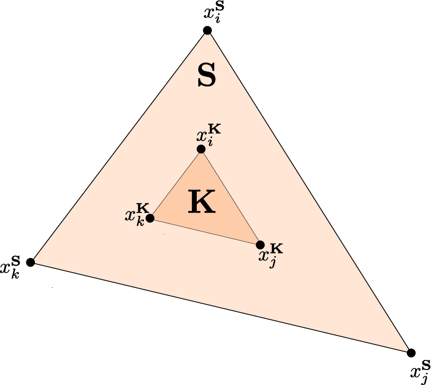
For any element 𝐊\mathbf{K}, we consider a domain 𝐒⊃𝐊\mathbf{S}\supset\mathbf{K} (see Figure 1), obtained from 𝐊\mathbf{K} by an homothetic transformation of center the centroid of 𝐊\mathbf{K}, and of ratio larger than 11.

Refer to caption
Figure 1: Definition of 𝐒\mathbf{S} (in 2D for clarity)

Let xj𝐒x^{\mathbf{S}}_{j} denote the coordinate of the vertex jj of the domain 𝐒\mathbf{S}. For any vertex ii of 𝐒\mathbf{S}, we introduce the affine function χi0,𝐒\chi^{0,\mathbf{S}}_{i} (defined on 𝐒\mathbf{S}) that satisfies the condition χi0,𝐒​(xj𝐒)=δi​j\chi^{0,\mathbf{S}}_{i}(x^{\mathbf{S}}_{j})=\delta_{ij} for all jj. Let χiε,𝐒∈H1​(𝐒)\chi^{\varepsilon,\mathbf{S}}_{i}\in H^{1}(\mathbf{S}) be the unique solution to the problem

−div[Aε(x)∇χiε,𝐒(x)]=0in 𝐒,χiε,𝐒=χi0,𝐒on ∂𝐒,-\mbox{div}\left[A^{\varepsilon}(x)\nabla\chi^{\varepsilon,\mathbf{S}}_{i}(x)\right]=0\ \ \mbox{in $\mathbf{S}$},\quad\chi^{\varepsilon,\mathbf{S}}_{i}=\chi^{0,\mathbf{S}}_{i}\ \ \mbox{on $\partial\mathbf{S}$}, (10)

which, in practice, is numerically solved e.g. using a finite element method with a mesh size adapted to the small scale ε\varepsilon. We then define the local basis functions

ϕiε,𝐊=∑j=1d+1αi​j​χjε,𝐒|𝐊\phi_{i}^{\varepsilon,\mathbf{K}}=\sum\limits_{j=1}^{d+1}\alpha_{ij}\left.\chi^{\varepsilon,\mathbf{S}}_{j}\right|_{\mathbf{K}} (11)

as linear combinations of the restrictions of χiε,𝐒\chi^{\varepsilon,\mathbf{S}}_{i} on 𝐊\mathbf{K}, with αi​j\alpha_{ij} chosen such that

∀1≤i,j≤d+1,ϕi0,𝐊​(xj𝐊)=∑j=1d+1αi​j​χj0,𝐒​(xj𝐊)=δi​j,\forall 1\leq i,j\leq d+1,\quad\phi_{i}^{0,\mathbf{K}}(x^{\mathbf{K}}_{j})=\sum\limits_{j=1}^{d+1}\alpha_{ij}\chi^{0,\mathbf{S}}_{j}(x^{\mathbf{K}}_{j})=\delta_{ij}, (12)

where xj𝐊x^{\mathbf{K}}_{j} denotes the coordinate of the jjth vertex of the element 𝐊\mathbf{K}. Note that the condition (12) is enforced on the function ϕi0,𝐊\phi_{i}^{0,\mathbf{K}}, and not on ϕiε,𝐊\phi_{i}^{\varepsilon,\mathbf{K}}. The coefficients αi​j\alpha_{ij} are consequently independent from ε\varepsilon. As ϕi0,𝐊\phi_{i}^{0,\mathbf{K}} and χj0,𝐒|𝐊\left.\chi^{0,\mathbf{S}}_{j}\right|_{\mathbf{K}} are both affine on 𝐊\mathbf{K}, condition (12) implies that

∀1≤i≤d+1,∀x∈𝐊,ϕi0,𝐊​(x)=∑j=1d+1αi​j​χj0,𝐒​(x).\forall 1\leq i\leq d+1,\quad\forall x\in\mathbf{K},\quad\phi_{i}^{0,\mathbf{K}}(x)=\sum\limits_{j=1}^{d+1}\alpha_{ij}\chi^{0,\mathbf{S}}_{j}(x). (13)

We next introduce the functions ϕiε\phi_{i}^{\varepsilon} defined on 𝒟{\mathcal{D}} by ϕiε|𝐊=ϕiε,𝐊\left.\phi_{i}^{\varepsilon}\right|_{\mathbf{K}}=\phi_{i}^{\varepsilon,\mathbf{K}} for all elements 𝐊\mathbf{K}.

Note that the problems (10), indexed by 𝐒\mathbf{S}, are all independent from one another. They may be solved in parallel.

Macroscale problem

We now introduce the finite dimensional space

𝒲h:=span​(ϕiε,i=1,⋯,L),\mathcal{W}_{h}:=\mbox{span}(\phi_{i}^{\varepsilon},\ i=1,\cdots,L),

and proceed with the approximation

Find uM∈𝒲h such that, for any v∈𝒲h, 𝒜εh​(uM,v)=b⁡(v),\mbox{Find $u_{M}\in\mathcal{W}_{h}$ such that, for any $v\in\mathcal{W}_{h}$, \hskip 10.22217pt${\cal A}^{h}_{\varepsilon}(u_{M},v)=b(v)$}, (14)

of (4), where

𝒜εh(u,v)=∑𝐊∫𝐊(∇v(x))TAε(x)∇u(x)dx and b(v)=∫𝒟f(x)v(x)dx.{\cal A}^{h}_{\varepsilon}(u,v)=\sum_{\mathbf{K}}\int_{\mathbf{K}}(\nabla v(x))^{T}A^{\varepsilon}(x)\nabla u(x)\,dx\ \mbox{ and }\ b(v)=\int_{\mathcal{D}}f(x)\>v(x)\,dx.

Observe that ϕiε\phi_{i}^{\varepsilon} has jumps across the edges of the triangulation (due to the use of the oversampling technique), hence 𝒲h⊄H1​(𝒟)\mathcal{W}_{h}\not\subset H^{1}(\mathcal{D}), thus the broken integral used to define 𝒜εh​(u,v){\cal A}^{h}_{\varepsilon}(u,v). On the other hand, since 𝒲h⊂L2​(𝒟)\mathcal{W}_{h}\subset L^{2}(\mathcal{D}), the linear form bb is well defined for v∈𝒲hv\in\mathcal{W}_{h}. The formulation (14) is a non-conforming Galerkin approximation of (4). This brings additional error terms in the error estimation (see Lemma 12 in Section 4). On another note, remark that the dimension of 𝒲h\mathcal{W}_{h} is equal to LL. The formulation (14) hence requires solving a linear system with only a limited number of degrees of freedom.

We are now in position to substantiate our claim in the introduction, where we briefly mentioned that, in the stochastic setting, a direct application of the MsFEM to approximate the solution to (2) is unpractical. It would indeed lead to compute, for each realization of Aε​(x,ω)A^{\varepsilon}(x,\omega), first a basis set and second a macroscale solution. This approach has been briefly examined theoretically in [21]. It is prohibitively expensive. We therefore turn to an alternate approach.

2.2 A weakly stochastic setting

We now restrict the general setting and propose a dedicated, practical MsFEM type approach. Following up on previous works (see [5, 13, 24, 41]) and as announced in (3), we assume here that the random matrix Aε​(x,ω)A^{\varepsilon}(x,\omega) in (2) is a perturbation of a deterministic matrix, in the sense that

Aε​(x,ω)≡Aηε​(x,ω)=A0ε​(x)+η​A1ε​(x,ω),A^{\varepsilon}(x,\omega)\equiv A^{\varepsilon}_{\eta}(x,\omega)=A_{0}^{\varepsilon}(x)+\eta\>A^{\varepsilon}_{1}(x,\omega), (15)

where η∈ℝ\eta\in\mathbb{R} is a small deterministic parameter, A0εA^{\varepsilon}_{0} and A1εA^{\varepsilon}_{1} are bounded matrices, and A0εA^{\varepsilon}_{0} is coercive, uniformly in ε\varepsilon. We also assume that the matrix AηεA_{\eta}^{\varepsilon} itself satisfies the coercivity and boundedness assumptions, uniformly in η\eta and ε\varepsilon (we refer to [6, 7, 8] and [15, 25] for other perturbative settings).

The principle of the proposed approach is to compute the MsFEM basis set of functions with the deterministic part A0εA^{\varepsilon}_{0} of the matrix AηεA^{\varepsilon}_{\eta}, and next to perform Monte-Carlo realizations for the macroscale problem (2)-(15), where we keep the exact matrix AηεA^{\varepsilon}_{\eta} (and not only its deterministic part). Following the approach sketched in Section 2.1, we first solve (10), with Aε​(x)≡A0ε​(x)A^{\varepsilon}(x)\equiv A_{0}^{\varepsilon}(x), and build the deterministic finite dimensional space

𝒲h:=span​(ϕiε,i=1,⋯,L)\mathcal{W}_{h}:=\mbox{span}(\phi_{i}^{\varepsilon},\ i=1,\cdots,L)

following (11)-(12). We next proceed with a standard Galerkin approximation of (2)-(15) using 𝒲h\mathcal{W}_{h}. For each m∈{1,⋯,M}m\in\{1,\cdots,M\}, we consider a realization Aηε,m​(⋅,ω)A^{\varepsilon,m}_{\eta}(\cdot,\omega) and compute uSm​(⋅,ω)∈𝒲hu^{m}_{S}(\cdot,\omega)\in\mathcal{W}_{h} such that

∀v∈𝒲h,∑𝐊∫𝐊(∇v(x))TAηε,m(x,ω)∇uSm(x,ω)dx=∫𝒟f(x)v(x)dx.\forall v\in\mathcal{W}_{h},\quad\sum\limits_{\mathbf{K}}\int_{\mathbf{K}}(\nabla v(x))^{T}A^{\varepsilon,m}_{\eta}(x,\omega)\nabla u^{m}_{S}(x,\omega)\,dx=\int_{\mathcal{D}}f(x)\>v(x)\,dx. (16)

Since the MsFEM basis functions are only computed once (rather than for each realization of Aηε​(x,ω)A^{\varepsilon}_{\eta}(x,\omega)), a large computational gain is expected, and obtained, in comparison to the direct approach described above.

3 Numerical simulations

This section is devoted to the many numerical simulations we have performed. We first discuss some implementation details. Next, we numerically estimate the performance of our approach on various test cases, and assess its sensitivity with respect to the magnitude of η\eta. We consider in Section 3.2 a test case in dimension one. In Section 3.3, we next study two test cases in dimension two. We also study how the presence in A1εA_{1}^{\varepsilon} (the random component of the matrix AηεA^{\varepsilon}_{\eta}) of high frequencies that are not present in the deterministic component A0εA_{0}^{\varepsilon}, and that are thus not encoded in the highly oscillatory basis functions, affects the accuracy of our approach.

Let uηεu^{\varepsilon}_{\eta} be the reference solution to (2)-(3) obtained using a finite element method with a mesh size adapted to the small scale ε\varepsilon, uSu_{S} be the approximation given by our approach (described in Section 2.2) and uMu_{M} be the approximation given by the direct approach (in which the MsFEM basis set is recomputed for each realization Aηε,m​(x,ω)A^{\varepsilon,m}_{\eta}(x,\omega), as explained at the end of Section 2.1). Our goal is to compare the error uS−uηεu_{S}-u_{\eta}^{\varepsilon} of our numerical approximation with the error uM−uηεu_{M}-u_{\eta}^{\varepsilon} of the direct and expensive approach. When η\eta is small, we expect the approximation uSu_{S} to be essentially as accurate as the approximation uMu_{M}, and we show below that this is indeed the case.

In the sequel, we assess the accuracy using the estimators

eL2​(u1,u2)=𝔼⁡(‖u1−u2‖L2​(𝒟)‖u2‖L2​(𝒟))andeH1​(u1,u2)=𝔼⁡(‖u1−u2‖Hh1‖u2‖Hh1),e_{L^{2}}(u_{1},u_{2})=\mathbb{E}\left(\frac{\|u_{1}-u_{2}\|_{L^{2}({\cal D})}}{\|u_{2}\|_{L^{2}({\cal D})}}\right)\quad\text{and}\quad e_{H^{1}}(u_{1},u_{2})=\mathbb{E}\left(\frac{\|u_{1}-u_{2}\|_{{H^{1}_{h}}}}{\|u_{2}\|_{{H^{1}_{h}}}}\right), (17)

where u1u_{1} and u2u_{2} are the solutions obtained with any two different methods, and

‖u‖Hh1:=(∑𝐊∈𝒯h‖u‖H1​(𝐊)2)1/2\|u\|_{H^{1}_{h}}:=\left(\sum\limits_{\mathbf{K}\in\mathcal{T}_{h}}\|u\|^{2}_{H^{1}(\mathbf{K})}\right)^{1/2} (18)

is the broken H1H^{1} norm. The expectation is in turn computed using a Monte-Carlo method. Considering MM realizations {Xm​(ω)}1≤m≤M\left\{X_{m}(\omega)\right\}_{1\leq m\leq M} of a random variable, e.g. X⁡(ω)=‖u1​(⋅,ω)−u2​(⋅,ω)‖Hh1‖u2​(⋅,ω)‖Hh1\displaystyle X(\omega)=\frac{\|u_{1}(\cdot,\omega)-u_{2}(\cdot,\omega)\|_{{H^{1}_{h}}}}{\|u_{2}(\cdot,\omega)\|_{{H^{1}_{h}}}}, we compute the empirical mean μM\mu_{M} and the empirical standard deviation σM\sigma_{M} as

μM​(X)=1M​∑m=1MXm​(ω),σM2​(X)=1M−1​∑m=1M(Xm​(ω)−μM​(X))2.\mu_{M}(X)=\frac{1}{M}\sum\limits_{m=1}^{M}X_{m}(\omega),\quad\quad\sigma_{M}^{2}(X)=\frac{1}{M-1}\sum\limits_{m=1}^{M}\left(X_{m}(\omega)-\mu_{M}(X)\right)^{2}. (19)

As a classical consequence of the Central Limit Theorem, the following estimate is commonly employed:

|𝔼⁡(X)−μM​(X)|≤1.96​σMM.\left|\mathbb{E}(X)-\mu_{M}(X)\right|\leq 1.96\frac{\sigma_{M}}{\sqrt{M}}.

It provides a practical evaluation of 𝔼⁡(X)\mathbb{E}(X) from the knowledge of μM​(X)\mu_{M}(X) and σM​(X)\sigma_{M}(X). The numerical parameters have been determined by an empirical study of convergence. For instance, for the reference solution, we choose the mesh size hh such that the quantity ‖uηε,h−uηε,h/2‖H1​(𝒟)‖uηε,h/2‖H1​(𝒟)\displaystyle\frac{\|u_{\eta}^{\varepsilon,h}-u_{\eta}^{\varepsilon,h/2}\|_{H^{1}({\cal D})}}{\|u_{\eta}^{\varepsilon,h/2}\|_{H^{1}({\cal D})}} is smaller than 0.03 %, thereby formally admitting that the approximation has converged in hh. The MsFEM parameters are determined likewise.

All the computations have been performed using FreeFem++ [33], with the MPI tools.

3.1 Implementation details

In the deterministic version of the MsFEM, the same matrix AεA^{\varepsilon} appears in the definition (10) of the basis functions and in the macroscale variational formulation (14). This can be used to expedite the computation of the stiffness matrix associated with (14). In our approach, described in Section 2.2, the matrix that appears in the definition of the basis functions is A0εA_{0}^{\varepsilon}, whereas the macroscale variational problem involves Aηε≡A0ε+η​A1εA^{\varepsilon}_{\eta}\equiv A_{0}^{\varepsilon}+\eta A^{\varepsilon}_{1}. An additional numerical computation is thus needed.

To solve (16), we need to compute, for each element 𝐊\mathbf{K} and each realization Aηε,m¯​(x,ω)A^{\varepsilon,\overline{m}}_{\eta}(x,\omega), the integrals

𝒦i​jη,m¯(ω)=∫𝐊(∇ϕiε,𝐊(x))TAηε,m¯(x,ω)∇ϕjε,𝐊(x)dx,\mathcal{K}^{\eta,\overline{m}}_{ij}(\omega)=\int_{\mathbf{K}}\left(\nabla\phi^{\varepsilon,\mathbf{K}}_{i}(x)\right)^{T}A^{\varepsilon,\overline{m}}_{\eta}(x,\omega)\nabla\phi^{\varepsilon,\mathbf{K}}_{j}(x)\,dx, (20)

where ϕiε,𝐊\phi_{i}^{\varepsilon,\mathbf{K}} are deterministic functions. We recall that Aηε​(x,ω)=A0ε​(x)+η​A1ε​(x,ω)A^{\varepsilon}_{\eta}(x,\omega)=A_{0}^{\varepsilon}(x)+\eta A^{\varepsilon}_{1}(x,\omega) (see (15)). To allow for an efficient evaluation of (20), we assume henceforth that A1εA^{\varepsilon}_{1} is of the form

A1ε​(x,ω)=∑k∈ℤd𝟏Q+k​(xε)​Xk​(ω)​Bεk​(x),A^{\varepsilon}_{1}(x,\omega)=\sum\limits_{k\in\mathbb{Z}^{d}}\mathbf{1}_{Q+k}\left(\frac{x}{\varepsilon}\right)\ X_{k}(\omega)\ B^{k}_{\varepsilon}(x), (21)

where Q=(0,1)dQ=(0,1)^{d}, where (Xk)k∈ℤd\left(X_{k}\right)_{k\in\mathbb{Z}^{d}} are scalar random variables, and for any k∈ℤdk\in\mathbb{Z}^{d}, x↦Bεk​(x)∈ℝd×dx\mapsto B^{k}_{\varepsilon}(x)\in\mathbb{R}^{d\times d} are some deterministic functions. We comment on this assumption in Remark 2 below. The important consequence of (21) is that we can write the integral (20) as a linear combination of deterministic integrals over cells of size ε\varepsilon, with random coefficients. To simplify the notation, we assume that the spatial dimension is d=2d=2. We define

p=⌊min⁡(yiε,yjε,ykε)⌋,q=⌊max⁡(yiε,yjε,ykε)⌋+1,p=\left\lfloor\min\left(\frac{y_{i}}{\varepsilon},\frac{y_{j}}{\varepsilon},\frac{y_{k}}{\varepsilon}\right)\right\rfloor,\quad q=\left\lfloor\max\left(\frac{y_{i}}{\varepsilon},\frac{y_{j}}{\varepsilon},\frac{y_{k}}{\varepsilon}\right)\right\rfloor+1,

and likewise, we define the integers ll and mm (see Fig. 2). We can then write (20) as

𝒦i​jη,m¯(ω)=∫𝐊(∇ϕiε,𝐊(x))TAηε,m¯(x,ω)∇ϕjε,𝐊(x)dx=𝒦i​j0,𝐊+η∑α=pq−1∑β=lm−1Xα,βm¯(ω)𝒦α​β​i​j1,𝐊,\mathcal{K}^{\eta,\overline{m}}_{ij}(\omega)=\int_{\mathbf{K}}\left(\nabla\phi^{\varepsilon,\mathbf{K}}_{i}(x)\right)^{T}A^{\varepsilon,\overline{m}}_{\eta}(x,\omega)\nabla\phi^{\varepsilon,\mathbf{K}}_{j}(x)\,dx=\mathcal{K}^{0,\mathbf{K}}_{ij}+\eta\sum\limits_{\alpha=p}^{q-1}\sum\limits_{\beta=l}^{m-1}X^{\overline{m}}_{\alpha,\beta}(\omega)\mathcal{K}^{1,\mathbf{K}}_{\alpha\beta ij}, (22)

where

𝒦i​j0,𝐊\displaystyle\mathcal{K}^{0,\mathbf{K}}_{ij} =\displaystyle= ∫𝐊(∇ϕiε,𝐊(x))TA0ε(x)∇ϕjε,𝐊(x)dx,\displaystyle\int_{\mathbf{K}}\left(\nabla\phi^{\varepsilon,\mathbf{K}}_{i}(x)\right)^{T}A_{0}^{\varepsilon}(x)\nabla\phi^{\varepsilon,\mathbf{K}}_{j}(x)\,dx, (23)
𝒦α​β​i​j1,𝐊\displaystyle\mathcal{K}^{1,\mathbf{K}}_{\alpha\beta ij} =\displaystyle= ∫α​ε(α+1)​ε∫β​ε(β+1)​ε𝟏𝐊(x)(∇ϕiε,𝐊(x))TBεk(x)∇ϕjε,𝐊(x)dx.\displaystyle\int\limits_{\alpha\varepsilon}^{(\alpha+1)\varepsilon}\int\limits_{\beta\varepsilon}^{(\beta+1)\varepsilon}\!\!\!\mathbf{1}_{\mathbf{K}}(x)\left(\nabla\phi^{\varepsilon,\mathbf{K}}_{i}(x)\right)^{T}B_{\varepsilon}^{k}(x)\nabla\phi^{\varepsilon,\mathbf{K}}_{j}(x)\,dx. (24)
Refer to caption
Figure 2: To practically compute the integral (20), we write that each element 𝐊\mathbf{K} (here in dimension d=2d=2) is a subset of a quadrangle (here [l​ε,m​ε]×[p​ε,q​ε][l\varepsilon,m\varepsilon]\times[p\varepsilon,q\varepsilon]) composed of cells of size εd\varepsilon^{d}.

We thus compute once the deterministic integrals (23) and (24). Next, for each realization of AηεA^{\varepsilon}_{\eta}, we evaluate the stiffness matrix elements 𝒦i​jη,m¯​(ω)\mathcal{K}^{\eta,\overline{m}}_{ij}(\omega) using the right hand side of (22). No numerical quadrature is needed. As a consequence of (21), most of the work for assembling the stiffness matrix is only performed once, independently of the number of Monte Carlo realizations. This significantly contributes to the gain in term of computational cost.

Remark 2.

Assumption (21) is quite general, and already covers many interesting cases in practice. As explained above, the point in (21) is that A1εA_{1}^{\varepsilon} is a direct product (or here, a sum of direct products) of a function depending on xx with a random variable that only depends on ω\omega. Otherwise stated, A1ε​(x,ω)A_{1}^{\varepsilon}(x,\omega) depends linearly, in an explicit way, of ω\omega. A similar assumption is made when applying reduced basis methods [45] to a problem of the type

Find uλu_{\lambda} such that, for any vv, a⁡(uλ,v,λ)=b⁡(v)a(u_{\lambda},v;\lambda)=b(v), (25)

where a⁡(⋅,⋅,λ)a(\cdot,\cdot;\lambda) is a bilinear form parameterized by λ\lambda. Assume this problem has been solved for some values {λi}i=1I\left\{\lambda_{i}\right\}_{i=1}^{I} of the parameter, yielding the functions {uλi}i=1I\left\{u_{\lambda_{i}}\right\}_{i=1}^{I}. Under the assumption that a⁡(⋅,⋅,λ)=a0​(⋅,⋅)+λ​a1​(⋅,⋅)a(\cdot,\cdot;\lambda)=a_{0}(\cdot,\cdot)+\lambda a_{1}(\cdot,\cdot) (namely, a⁡(⋅,⋅,λ)a(\cdot,\cdot;\lambda) depends linearly on λ\lambda), one can precompute the stiffness matrix elements a0​(uλi,uλj)a_{0}(u_{\lambda_{i}},u_{\lambda_{j}}) and a1​(uλi,uλj)a_{1}(u_{\lambda_{i}},u_{\lambda_{j}}) for any 1≤i,j≤I1\leq i,j\leq I. This allows to next perform a very efficient Galerkin approximation of the problem (25) (for any λ\lambda) on the space Span​(uλi,i=1,⋯,I)\text{Span}(u_{\lambda_{i}},i=1,\cdots,I).

3.2 One-dimensional test-case

The purpose of this section is threefold. We first calibrate the number MM of realizations considered for the Monte-Carlo method for the two-dimensional numerical experiments that we consider in the sequel. We next investigate how the accuracy of our approach depends on η\eta and on the presence of frequencies in the random coefficient aηεa^{\varepsilon}_{\eta} that are not taken into account in the MsFEM basis set functions. The low computational costs that we face in this one-dimensional situation allow us to test our approach more comprehensively than in the two-dimensional test-cases described below.

Let (Xk)k∈ℤ\left(X_{k}\right)_{k\in\mathbb{Z}} denote a sequence of independent, identically distributed scalar random variables uniformly distributed in [0,1][0,1]. We consider the random coefficient

aηε(x,ω)=∑k∈ℤ𝟏(k,k+1](xε)(5+50sin2(π​xε)+ηXk(ω)κsin2(ζ​π​xε)),a^{\varepsilon}_{\eta}(x,\omega)=\sum\limits_{k\in\mathbb{Z}}\mathbf{1}_{(k,k+1]}\left(\frac{x}{\varepsilon}\right)\,\left(5+50\sin^{2}\left(\frac{\pi x}{\varepsilon}\right)+\eta X_{k}(\omega)\>\kappa\>\sin^{2}\left(\frac{\zeta\pi x}{\varepsilon}\right)\right),

which is a particular example of the expansion (15) with

a0ε(x)=5+50sin2(π​xε)anda1ε(x,ω)=∑k∈ℤ𝟏(k,k+1](xε)Xk(ω)κsin2(ζ​π​xε),a_{0}^{\varepsilon}(x)=5+50\sin^{2}\left(\frac{\pi x}{\varepsilon}\right)\quad\text{and}\quad a^{\varepsilon}_{1}(x,\omega)=\sum\limits_{k\in\mathbb{Z}}\mathbf{1}_{(k,k+1]}\left(\frac{x}{\varepsilon}\right)\ X_{k}(\omega)\ \kappa\>\sin^{2}\left(\frac{\zeta\pi x}{\varepsilon}\right),

and that satisfies the structural assumption (21). We set ε=0.025\varepsilon=0.025 and choose κ\kappa such that the quantity

𝒦⁡(κ,ζ)=‖a1εa0ε‖L∞​(𝒟×Ω)=SupEssω∈Ω​‖a1ε​(⋅,ω)a0ε​(⋅,ω)‖L∞​(𝒟)\mathcal{K}(\kappa,\zeta)=\left\|\frac{a^{\varepsilon}_{1}}{a_{0}^{\varepsilon}}\right\|_{L^{\infty}({\cal D}\times\Omega)}=\text{SupEss}_{\omega\in\Omega}\left\|\frac{a^{\varepsilon}_{1}(\cdot,\omega)}{a_{0}^{\varepsilon}(\cdot,\omega)}\right\|_{L^{\infty}({\cal D})} (26)

has the same value 𝒦=1\mathcal{K}=1 for the three different values of ζ={1,3,7}\zeta=\{1,3,7\} we consider below. We analytically compute the reference function uηεu_{\eta}^{\varepsilon}, solution to

−dd​x​(aηε​(x,ω)​d​uηεd​x​(x,ω))=1in (0,1),uηε​(0,ω)=uηε​(1,ω)=0,-\frac{d}{dx}\left(a^{\varepsilon}_{\eta}\left(x,\omega\right)\frac{du_{\eta}^{\varepsilon}}{dx}(x,\omega)\right)=1\ \ \mbox{in $(0,1)$},\quad u_{\eta}^{\varepsilon}(0,\omega)=u_{\eta}^{\varepsilon}(1,\omega)=0,

as well as the MsFEM basis functions for both approaches. Let uMu_{M} and uSu_{S} be the approximation of uηεu_{\eta}^{\varepsilon} by the two MsFEM approaches described above, where the coarse mesh size is h=1/30h=1/30.

We first calibrate the number of independent realizations to accurately approximate the exact expectation in (17) by the empirical mean (19). To this aim, we present on Fig. 3 the mean and the confidence interval computed using (19) for an increasing number MM of realizations (we compute up to 1000 independent realizations). We check that this indicator reaches a plateau for M≥30M\geq 30, and thus converges fast. On this example, considering 30 realizations is hence sufficient to accurately compute the error (17). Based on this observation, we will only consider M=30M=30 realizations in the two dimensional examples of Section 3.3.

Refer to caption
Figure 3: Convergence of the indicator eH1​(uM,uηε)e_{H^{1}}(u_{M},u_{\eta}^{\varepsilon}) (see (17)), for η=1\eta=1, ζ=1\zeta=1 and κ=55\kappa=55. For each value of MM, we plot the empirical mean along with its confidence interval, computed from the first MM realizations. We only plot the results for the first 5050 realizations.
Remark 3.

There is no reason to think that the calibration of our parameters that we perform in the one-dimensional situation provides an adequate adaptation of these parameters for the higher dimensional setting. We however see no other manner to proceed and the approach has indeed provided us with good results.

Note also that the MsFEM approach is much more accurate in the one-dimensional setting than in the two-dimensional setting (compare Tables 3, 3 and 3 with Tables 12 and 12 below). This is due to the specificity of the one dimensional setting. However, one-dimensional examples remain relevant for e.g. assessing how the MsFEM accuracy depends on η\eta.

We now check how the accuracy of our approach depends on η\eta. In Tables 3, 3, 3, 6, 6 and 6, we report the estimators (17), along with their confidence intervals, for various choices of (κ,ζ)(\kappa,\zeta) that all correspond to 𝒦⁡(κ,ζ)=1\mathcal{K}(\kappa,\zeta)=1. For η≤0.1\eta\leq 0.1, we observe that ‖uS−uηε‖\|u_{S}-u_{\eta}^{\varepsilon}\| and ‖uM−uηε‖\|u_{M}-u_{\eta}^{\varepsilon}\| are of the same order of magnitude, and are both larger than ‖uM−uS‖\|u_{M}-u_{S}\| (both in L2L^{2} and broken H1H^{1} norms). We thus obtain the same accuracy with the direct and the weak stochastic MsFEM approaches, whereas the weak stochastic MsFEM is computationally (much) less expensive. For η=1\eta=1, as expected, the accuracy of the approximation uSu_{S} deteriorates. The accuracy of uMu_{M} is independent of η\eta.

Remark 4.

In Section 4, we estimate in the H1H^{1} (broken) norm the error between the reference solution uηεu_{\eta}^{\varepsilon} and the weak MsFEM solution uSu_{S}. For information, we also include in Tables 3–6 the numerical comparison in the L2L^{2} norm.

Table 1: H1​(0,1)H^{1}(0,1) error (17) (in %) for κ=55\kappa=55 and ζ=1\zeta=1
η\eta eH1​(uM,uηε)e_{H^{1}}(u_{M},u_{\eta}^{\varepsilon}) eH1​(uS,uηε)e_{H^{1}}(u_{S},u_{\eta}^{\varepsilon}) eH1​(uS,uM)e_{H^{1}}(u_{S},u_{M})
11 0.14644±0.000360.14644\pm 0.00036 2.62550±0.026962.62550\pm 0.02696 2.44359±0.026962.44359\pm 0.02696
0.10.1 0.16001±0.000060.16001\pm 0.00006 0.15021±0.000510.15021\pm 0.00051 0.07036±0.000440.07036\pm 0.00044
0.010.01 0.16258±0.000000.16258\pm 0.00000 0.10837±0.000020.10837\pm 0.00002 0.04825±0.000250.04825\pm 0.00025
Table 2: H1​(0,1)H^{1}(0,1) error (17) (in %) for κ=14.38\kappa=14.38 and ζ=3\zeta=3
η\eta eH1​(uM,uηε)e_{H^{1}}(u_{M},u_{\eta}^{\varepsilon}) eH1​(uS,uηε)e_{H^{1}}(u_{S},u_{\eta}^{\varepsilon}) eH1​(uS,uM)e_{H^{1}}(u_{S},u_{M})
11 0.18269±0.000300.18269\pm 0.00030 2.38950±0.022772.38950\pm 0.02277 2.23869±0.022302.23869\pm 0.02230
0.10.1 0.16529±0.000030.16529\pm 0.00003 0.14959±0.000550.14959\pm 0.00055 0.08082±0.000410.08082\pm 0.00041
0.010.01 0.16314±0.000000.16314\pm 0.00000 0.10840±0.000000.10840\pm 0.00000 0.04954±0.000010.04954\pm 0.00001
Table 3: H1​(0,1)H^{1}(0,1) error (17) (in %) for κ=8.39\kappa=8.39 and ζ=7\zeta=7
η\eta eH1​(uM,uηε)e_{H^{1}}(u_{M},u_{\eta}^{\varepsilon}) eH1​(uS,uηε)e_{H^{1}}(u_{S},u_{\eta}^{\varepsilon}) eH1​(uS,uM)e_{H^{1}}(u_{S},u_{M})
11 0.17436±0.000260.17436\pm 0.00026 2,34495±0.021052,34495\pm 0.02105 2,27358±0.020892,27358\pm 0.02089
0.10.1 0.16465±0.000040.16465\pm 0.00004 0.15748±0.000670.15748\pm 0.00067 0.09803±0.000530.09803\pm 0.00053
0.010.01 0.16308±0.000000.16308\pm 0.00000 0.10846±0.000000.10846\pm 0.00000 0.05054±0.000010.05054\pm 0.00001
Table 4: L2​(0,1)L^{2}(0,1) error (17) (in %) for κ=55\kappa=55 and ζ=1\zeta=1
η\eta eL2​(uM,uηε)e_{L^{2}}(u_{M},u_{\eta}^{\varepsilon}) eL2​(uS,uηε)e_{L^{2}}(u_{S},u_{\eta}^{\varepsilon}) eL2​(uS,uM)e_{L^{2}}(u_{S},u_{M})
11 0.00018±0.000000.00018\pm 0.00000 0.07286±0.003170.07286\pm 0.00317 0.06861±0.003060.06861\pm 0.00306
0.10.1 0.00018±0.000000.00018\pm 0.00000 0.00045±0.000020.00045\pm 0.00002 0.00024±0.000010.00024\pm 0.00001
0.010.01 0.00018±0.000000.00018\pm 0.00000 0.00015±0.000000.00015\pm 0.00000 0.00002±0.000000.00002\pm 0.00000
Table 5: L2​(0,1)L^{2}(0,1) error (17) (in %) for κ=14.38\kappa=14.38 and ζ=3\zeta=3
η\eta eL2​(uM,uηε)e_{L^{2}}(u_{M},u_{\eta}^{\varepsilon}) eL2​(uS,uηε)e_{L^{2}}(u_{S},u_{\eta}^{\varepsilon}) eL2​(uS,uM)e_{L^{2}}(u_{S},u_{M})
11 0.00019±0.000000.00019\pm 0.00000 0.06658±0.002700.06658\pm 0.00270 0.06238±0.002610.06238\pm 0.00261
0.10.1 0.00018±0.000000.00018\pm 0.00000 0.00036±0.000010.00036\pm 0.00001 0.00019±0.000010.00019\pm 0.00001
0.010.01 0.00018±0.000000.00018\pm 0.00000 0.00015±0.000000.00015\pm 0.00000 0.00002±0.000000.00002\pm 0.00000
Table 6: L2​(0,1)L^{2}(0,1) error (17) (in %) for κ=8.39\kappa=8.39 and ζ=7\zeta=7
η\eta eL2​(uM,uηε)e_{L^{2}}(u_{M},u_{\eta}^{\varepsilon}) eL2​(uS,uηε)e_{L^{2}}(u_{S},u_{\eta}^{\varepsilon}) eL2​(uS,uM)e_{L^{2}}(u_{S},u_{M})
11 0.00018±0.000000.00018\pm 0.00000 0.08903±0.003100.08903\pm 0.00310 0.08410±0.002610.08410\pm 0.00261
0.10.1 0.00018±0.000000.00018\pm 0.00000 0.00037±0.000020.00037\pm 0.00002 0.00016±0.000000.00016\pm 0.00000
0.010.01 0.00018±0.000000.00018\pm 0.00000 0.00015±0.000000.00015\pm 0.00000 0.00003±0.000000.00003\pm 0.00000

We now turn to a different question. In the example considered here, some frequencies present in a1εa^{\varepsilon}_{1} do not appear in a0εa_{0}^{\varepsilon}, and are thus not captured in the highly oscillatory basis functions ϕiε\phi_{i}^{\varepsilon}. We now show that our approach can still handle this case, provided the amplitude of these modes remains small.

We first consider the case when the amplitude κ\kappa associated to the frequency ζ\zeta is kept constant, and compare the performance of our approach in the case ζ=1\zeta=1 and ζ=3\zeta=3. In the latter case, a relevant high frequency is not taken into account in the basis set functions. Comparing Tables 3 and 6 (corresponding to ζ=1\zeta=1) with Tables 8 and 8 (corresponding to ζ=3\zeta=3) for a given value of η\eta, we see that the accuracy of our approach deteriorates. This is not unexpected, of course. Otherwise stated, to achieve a given accuracy (say an error of 15 % in the broken H1H^{1} norm), we need to take smaller values of η\eta (namely η≤0.01\eta\leq 0.01) when ζ=3\zeta=3 than when ζ=1\zeta=1 (in which case η=0.1\eta=0.1 is already a sufficiently small value).

We now run the comparison differently. As we increase the gap between the frequency present in a1εa^{\varepsilon}_{1} and that present in a0εa^{\varepsilon}_{0} (i.e., as we increase ζ\zeta), we simultaneously decrease the amplitude κ\kappa of that mode. In practice, we do this by keeping constant the parameter 𝒦⁡(κ,ζ)\mathcal{K}(\kappa,\zeta) defined by (26). Then the accuracy of our approach remains constant, and is independent of ζ\zeta. See indeed the numerical results of Tables 3-6, that all correspond to the choice 𝒦⁡(κ,ζ)=1\mathcal{K}(\kappa,\zeta)=1, for three different values of ζ\zeta. We observe that, at fixed η\eta, errors are comparable, and independent of the value of (κ,ζ)(\kappa,\zeta).

In conclusion, the accuracy of our approach depends both on the amplitude κ\kappa and the value ζ\zeta of the high frequency not taken into account in the MsFEM basis set functions. If ζ\zeta and κ\kappa are scaled so that 𝒦⁡(κ,ζ)\mathcal{K}(\kappa,\zeta) remains constant (which implies that κ\kappa decreases if ζ\zeta increases), then the accuracy of our approach remains constant.

Table 7: H1​(0,1)H^{1}(0,1) error (17) (in %) for κ=55\kappa=55 and ζ=3\zeta=3
η\eta eH1​(uM,uηε)e_{H^{1}}(u_{M},u_{\eta}^{\varepsilon}) eH1​(uS,uηε)e_{H^{1}}(u_{S},u_{\eta}^{\varepsilon}) eH1​(uS,uM)e_{H^{1}}(u_{S},u_{M})
11 0.21826±0.000730.21826\pm 0.00073 12.30047±0.1064712.30047\pm 0.10647 12.01694±0.1061712.01694\pm 0.10617
0.10.1 0.17142±0.000130.17142\pm 0.00013 0.59293±0.005190.59293\pm 0.00519 0.49523±0.004890.49523\pm 0.00489
0.010.01 0.16383±0.000010.16383\pm 0.00001 0.11448±0.000140.11448\pm 0.00014 0.05247±0.000070.05247\pm 0.00007
Table 8: L2​(0,1)L^{2}(0,1) error (17) (in %) for κ=55\kappa=55 and ζ=3\zeta=3
η\eta eL2​(uM,uηε)e_{L^{2}}(u_{M},u_{\eta}^{\varepsilon}) eL2​(uS,uηε)e_{L^{2}}(u_{S},u_{\eta}^{\varepsilon}) eL2​(uS,uM)e_{L^{2}}(u_{S},u_{M})
11 0.00022±0.000000.00022\pm 0.00000 1.53780±0.038781.53780\pm 0.03878 1.51837±0.003851.51837\pm 0.00385
0.10.1 0.00019±0.000000.00019\pm 0.00000 0.00503±0.000270.00503\pm 0.00027 0.00406±0.000240.00406\pm 0.00024
0.010.01 0.00018±0.000000.00018\pm 0.00000 0.00018±0.000000.00018\pm 0.00000 0.00005±0.000000.00005\pm 0.00000

3.3 Two-dimensional test-cases

We now test our approach on two-dimensional test cases. Using the first test case, we show, similarly to the one-dimensional situation, that the weak stochastic MsFEM yields accurate results, provided the parameter η\eta is sufficiently small, and provided that the amplitude associated to frequencies present in AηεA^{\varepsilon}_{\eta} but not encoded in the deterministic basis functions is small (see Section 3.3.1). Next, in Section 3.3.2, we consider a test case similar to a classical benchmark test case of the literature. We again observe that our approach is efficient. For both cases, we show that the parameter η\eta does not need to be extremely small for our approach to be highly competitive.

3.3.1 A multi-frequency case

In line with what we observed in the one-dimensional case, we show here that the weak stochastic MsFEM provides interesting results even in the case when not all the frequencies present in AηεA^{\varepsilon}_{\eta} are captured in the deterministic basis functions, provided their amplitude is not too large. To this aim, we consider the following numerical example.

Let (Xk,l)(k,l)∈ℤ2\left(X_{k,l}\right)_{(k,l)\in\mathbb{Z}^{2}} denote a sequence of independent, identically distributed scalar random variables uniformly distributed in the interval [0,1][0,1]. We consider the random matrix

Aηε​(x,y,ω)=a0ε​(x,y)​Id2+η​a1ε​(x,y,ω)​Id2,A_{\eta}^{\varepsilon}(x,y,\omega)=a_{0}^{\varepsilon}(x,y)\ \text{Id}_{2}+\eta a_{1}^{\varepsilon}(x,y,\omega)\ \text{Id}_{2},

with

a0ε​(x,y)\displaystyle a_{0}^{\varepsilon}(x,y) =\displaystyle= 5+50​sin2⁡(π​xε)​sin2⁡(π​yε),\displaystyle 5+50\sin^{2}\left(\frac{\pi x}{\varepsilon}\right)\sin^{2}\left(\frac{\pi y}{\varepsilon}\right),
a1ε​(x,y,ω)\displaystyle a_{1}^{\varepsilon}(x,y,\omega) =\displaystyle= ∑(k,l)∈ℤ2𝟏(k,k+1](xε)𝟏(l,l+1](yε)(Xk,l(ω)κsin2(ζ​π​xε)sin2(ζ​π​yε)).\displaystyle\sum\limits_{(k,l)\in\mathbb{Z}^{2}}\mathbf{1}_{(k,k+1]}\left(\frac{x}{\varepsilon}\right)\mathbf{1}_{(l,l+1]}\left(\frac{y}{\varepsilon}\right)\left(X_{k,l}(\omega)\>\kappa\>\sin^{2}\left(\frac{\zeta\pi x}{\varepsilon}\right)\sin^{2}\left(\frac{\zeta\pi y}{\varepsilon}\right)\right).

Again, this choice is a particular example of the expansion (15) satisfying the structural assumption (21). We consider two different values of ζ\zeta, namely ζ=1\zeta=1 and ζ=3\zeta=3. As in the previous test case, the frequency ζ\zeta is not present in the deterministic part of AηεA^{\varepsilon}_{\eta}, and thus not encoded in the basis functions. In line with what we observed in Section 3.2, we choose the amplitude κ\kappa associated to that frequency such that the quantity (26) has the same value 𝒦=1\mathcal{K}=1 for both values of ζ\zeta. We compute uηεu_{\eta}^{\varepsilon} solution to

−div[Aηε(⋅,ω)∇uηε(⋅,ω)]=1in 𝒟,uηε(⋅,ω)=0 on ∂𝒟,-\mbox{div}\left[A_{\eta}^{\varepsilon}(\cdot,\omega)\,\nabla u_{\eta}^{\varepsilon}(\cdot,\omega)\right]=1\ \ \mbox{in $\mathcal{D}$},\quad u_{\eta}^{\varepsilon}(\cdot,\omega)=0\ \ \mbox{ on $\partial\mathcal{D}$},

on the domain 𝒟=(0,1)2\mathcal{D}=(0,1)^{2} with ε=0.025\varepsilon=0.025. Let uMu_{M} and uSu_{S} be its approximation by the two MsFEM approaches described above. The numerical parameters for the computation are again determined using an empirical study of convergence. We use for the reference solution uηεu^{\varepsilon}_{\eta} a fine mesh of size hf=ε/40h_{f}=\varepsilon/40. The MsFEM basis functions are computed in each element 𝐊\mathbf{K} using a mesh of size hM=ε/80h_{M}=\varepsilon/80. The oversampling parameter (i.e. the scale ratio of the homothetic transformation between 𝐊\mathbf{K} and 𝐒\mathbf{S}, see Fig. 1) is equal to 33. The coarse mesh size is h=1/30h=1/30. In view of the results of Section 3.2, we consider M=30M=30 independent realizations, which will prove to again be sufficient to obtain accurate results.

In Tables 12 and 12 (Tables 12 and 12 respectively), we report the estimator (17), along with its confidence interval, for the broken H1​(𝒟)H^{1}(\mathcal{D}) norm and for the L2​(𝒟)L^{2}(\mathcal{D}) norm, respectively. The results obtained here confirm our observations in the one-dimensional setting (Section 3.2):

  • •

    for given ζ\zeta and κ\kappa, we observe that, when η\eta is sufficiently small (here, η≤0.1\eta\leq 0.1), the alternative approach provides a solution uSu_{S} that is an approximation of uηεu_{\eta}^{\varepsilon} as accurate as uMu_{M}, for a much smaller computational cost (as the MsFEM basis set has only been computed once rather than for each independent realization of AηεA_{\eta}^{\varepsilon}).

  • •

    our approach yields accurate results even if the frequency ζ\zeta is not encoded in the basis functions ϕiε\phi_{i}^{\varepsilon}, provided the associated amplitude κ\kappa is scaled accordingly. Figures in Table 12 (respectively Table 12) are very close to those of Table 12 (respectively Table 12). This confirms that the error made by the weak stochastic MsFEM seems to be independent of κ\kappa and ζ\zeta, provided these two parameters are scaled so that 𝒦⁡(κ,ζ)\mathcal{K}(\kappa,\zeta) remains constant. If ζ\zeta becomes different than 1, the frequency present in a0εa_{0}^{\varepsilon}, then the amplitude κ\kappa associated to the frequency ζ\zeta has to decrease to keep 𝒦⁡(κ,ζ)\mathcal{K}(\kappa,\zeta) (and thus the accuracy of uSu_{S}) constant.

These observations again demonstrate the efficiency of the approach.

Table 9: H1​(𝒟)H^{1}(\mathcal{D}) error (17) (in %) for κ=73.61\kappa=73.61 and ζ=1\zeta=1
η\eta eH1​(uM,uηε)e_{H^{1}}(u_{M},u_{\eta}^{\varepsilon}) eH1​(uS,uηε)e_{H^{1}}(u_{S},u_{\eta}^{\varepsilon}) eH1​(uS,uM)e_{H^{1}}(u_{S},u_{M})
11 7.8437±0.13507.8437\pm 0.1350 19.8818±0.412319.8818\pm 0.4123 18.8662±0.421618.8662\pm 0.4216
0.10.1 6.8053±0.01656.8053\pm 0.0165 7.3868±0.02767.3868\pm 0.0276 3.1528±0.05173.1528\pm 0.0517
0.010.01 6.7338±0.00176.7338\pm 0.0017 6.9795±0.00166.9795\pm 0.0016 1.8763±0.00131.8763\pm 0.0013
Table 10: H1​(𝒟)H^{1}(\mathcal{D}) error (17) (in %) for κ=10\kappa=10 and ζ=3\zeta=3
η\eta eH1​(uM,uηε)e_{H^{1}}(u_{M},u_{\eta}^{\varepsilon}) eH1​(uS,uηε)e_{H^{1}}(u_{S},u_{\eta}^{\varepsilon}) eH1​(uS,uM)e_{H^{1}}(u_{S},u_{M})
11 6.7224±0.03686.7224\pm 0.0368 12.7292±0.217212.7292\pm 0.2172 10.8128±0.244210.8128\pm 0.2442
0.10.1 6.7154±0.00446.7154\pm 0.0044 7.1069±0.01287.1069\pm 0.0128 2.2925±0.02062.2925\pm 0.0206
0.010.01 6.1725±0.00046.1725\pm 0.0004 6.9770±0.00106.9770\pm 0.0010 1.8504±0.00031.8504\pm 0.0003
Table 11: L2​(𝒟)L^{2}(\mathcal{D}) error (17) (in %) for κ=73.61\kappa=73.61 and ζ=1\zeta=1
η\eta eL2​(uM,uηε)e_{L^{2}}(u_{M},u_{\eta}^{\varepsilon}) eL2​(uS,uηε)e_{L^{2}}(u_{S},u_{\eta}^{\varepsilon}) eL2​(uS,uM)e_{L^{2}}(u_{S},u_{M})
11 1.4355±0.07951.4355\pm 0.0795 4.1649±0.16524.1649\pm 0.1652 2.8468±0.16942.8468\pm 0.1694
0.10.1 1.0630±0.01081.0630\pm 0.0108 1.1369±0.00751.1369\pm 0.0075 0.1441±0.03540.1441\pm 0.0354
0.010.01 1.0211±0.00111.0211\pm 0.0011 1.1512±0.00071.1512\pm 0.0007 0.1351±0.00140.1351\pm 0.0014
Table 12: L2​(𝒟)L^{2}(\mathcal{D}) error (17) (in %) for κ=10\kappa=10 and ζ=3\zeta=3
η\eta eL2​(uM,uηε)e_{L^{2}}(u_{M},u_{\eta}^{\varepsilon}) eL2​(uS,uηε)e_{L^{2}}(u_{S},u_{\eta}^{\varepsilon}) eL2​(uS,uM)e_{L^{2}}(u_{S},u_{M})
11 1.0744±0.01271.0744\pm 0.0127 1.8433±0.05821.8433\pm 0.0582 0.8426±0.08320.8426\pm 0.0832
0.10.1 1.0226±0.00151.0226\pm 0.0015 1.1249±0.00381.1249\pm 0.0038 0.1147±0.00730.1147\pm 0.0073
0.010.01 1.0170±0.00011.0170\pm 0.0001 1.1551±0.00041.1551\pm 0.0004 0.1427±0.00030.1427\pm 0.0003
Remark 5.

In Tables 12-12, we observe that the size of the confidence interval is much smaller than the distance between two different errors. This a posteriori validates the choice of the number MM of Monte Carlo realizations according to the calibration we performed in the one-dimensional setting. In the two-dimensional setting studied here, we observe that considering M=30M=30 realizations is again sufficient. The same conclusion holds for results presented in Tables 14-16 below.

3.3.2 A classical test case

We consider in this section a test case similar to a classical test case of the literature (see e.g. [37, 39, 19, 32]). Let (Xk,l)(k,l)∈ℤ2\left(X_{k,l}\right)_{(k,l)\in\mathbb{Z}^{2}} denote a sequence of independent, identically distributed scalar random variables uniformly distributed in the interval [0,1][0,1]. We consider the random matrix

Aηε(x,y,ω)=∑(k,l)∈ℤ2𝟏(k,k+1](xε)𝟏(l,l+1](yε)(2+P​sin⁡(2​π​x/ε)2+P​sin⁡(2​π​y/ε)+2+sin⁡(2​π​y/ε)2+P​sin⁡(2​π​x/ε))(1+ηXk,l(ω))Id2,A_{\eta}^{\varepsilon}(x,y,\omega)=\sum\limits_{(k,l)\in\mathbb{Z}^{2}}\mathbf{1}_{(k,k+1]}\left(\frac{x}{\varepsilon}\right)\mathbf{1}_{(l,l+1]}\left(\frac{y}{\varepsilon}\right)\left(\frac{2+P\sin(2\pi x/\varepsilon)}{2+P\sin(2\pi y/\varepsilon)}+\frac{2+\sin(2\pi y/\varepsilon)}{2+P\sin(2\pi x/\varepsilon)}\right)\left(1+\eta X_{k,l}(\omega)\right)\ \text{Id}_{2},

with P=1.8P=1.8 and ε=0.025\varepsilon=0.025. We compute the reference solution uηεu_{\eta}^{\varepsilon} and its two approximations uMu_{M} and uSu_{S} with the same numerical parameters as in Section 3.3.1.

In Tables 14 and 14, we report the estimator (17), along with its confidence interval, for the broken H1​(𝒟)H^{1}(\mathcal{D}) norm and for the L2​(𝒟)L^{2}(\mathcal{D}) norm, respectively. We again see that, when η\eta is sufficiently small, uSu_{S} is an approximation of the reference solution uηεu^{\varepsilon}_{\eta} as accurate as uMu_{M}. In Tables 16 and 16, we report on the accuracy of uSu_{S}, for more values of η\eta. Assuming that the accuracy of uMu_{M} does not depend on η\eta (which is consistent with the results reported in Tables 14 and 14), we see that our approach is as accurate as the direct, expensive MsFEM approach, as soon as η≤0.1\eta\leq 0.1 (if we use the broken H1H^{1} norm to assess accuracy) and η≤0.25\eta\leq 0.25 (if we rather use the L2L^{2} norm). The parameter η\eta hence does not need to be extremely small for our approach to be highly competitive.

Table 13: H1​(𝒟)H^{1}(\mathcal{D}) error (17) (in %)
η\eta eH1​(uM,uηε)e_{H^{1}}(u_{M},u_{\eta}^{\varepsilon}) eH1​(uS,uηε)e_{H^{1}}(u_{S},u_{\eta}^{\varepsilon}) eH1​(uS,uM)e_{H^{1}}(u_{S},u_{M})
11 8.1154±0.19138.1154\pm 0.1913 17.3678±0.778417.3678\pm 0.7784 15.5113±0.868915.5113\pm 0.8689
0.10.1 7.1664±0.01997.1664\pm 0.0199 7.0524±0.07057.0524\pm 0.0705 2.5638±0.10062.5638\pm 0.1006
0.010.01 7.1453±0.00207.1453\pm 0.0020 7.2837±0.00677.2837\pm 0.0067 1.3882±0.00201.3882\pm 0.0020
Table 14: L2​(𝒟)L^{2}(\mathcal{D}) error (17) (in %\%)
η\eta eL2​(uM,uηε)e_{L^{2}}(u_{M},u_{\eta}^{\varepsilon}) eL2​(uS,uηε)e_{L^{2}}(u_{S},u_{\eta}^{\varepsilon}) eL2​(uS,uM)e_{L^{2}}(u_{S},u_{M})
11 0.5620±0.08030.5620\pm 0.0803 1.6855±0.48601.6855\pm 0.4860 1.4739±0.50481.4739\pm 0.5048
0.10.1 0.5354±0.01600.5354\pm 0.0160 0.5688±0.06300.5688\pm 0.0630 0.1984±0.07120.1984\pm 0.0712
0.010.01 0.5347±0.00120.5347\pm 0.0012 0.6192±0.00540.6192\pm 0.0054 0.1072±0.00320.1072\pm 0.0032
Table 15: H1​(𝒟)H^{1}(\mathcal{D}) error (17) (in %\%)
η\eta eH1​(uS,uηε)e_{H^{1}}(u_{S},u_{\eta}^{\varepsilon})
11 17.3678±0.778417.3678\pm 0.7784
0.50.5 15.9578±0.346115.9578\pm 0.3461
0.250.25 10.6130±0.159110.6130\pm 0.1591
0.10.1 7.0524±0.07057.0524\pm 0.0705
0.010.01 7.2837±0.00677.2837\pm 0.0067
Table 16: L2​(𝒟)L^{2}(\mathcal{D}) error (17) (in %\%)
η\eta eL2​(uS,uηε)e_{L^{2}}(u_{S},u_{\eta}^{\varepsilon})
11 1.6855±0.48601.6855\pm 0.4860
0.50.5 1.0246±0.44141.0246\pm 0.4414
0.250.25 0.5291±0.22850.5291\pm 0.2285
0.10.1 0.5688±0.06300.5688\pm 0.0630
0.010.01 0.6192±0.00540.6192\pm 0.0054

4 Analysis

This section is devoted to the analysis of the approach introduced in Section 2.2, and to the derivation of error bounds. As is often the case for the MsFEM (see e.g. [32]), we perform the analysis in a setting where the problem (2)-(3) that we consider admits a homogenized limit as ε\varepsilon vanishes (although, we repeat it, the approach is used in practice for more general cases). The structure of our proof is similar to that for the deterministic setting, which we now overview (we refer to [32] for all the details).

In the case when the oversampling technique is not used, the MsFEM is a conforming Galerkin approximation, and the error is estimated using the Céa lemma:

‖uε−uM‖H1≤C​infvh∈𝒲h‖uε−vh‖H1,\|u^{\varepsilon}-u_{M}\|_{H^{1}}\leq C\inf\limits_{v_{h}\in\mathcal{W}_{h}}\|u^{\varepsilon}-v_{h}\|_{H^{1}},

where uεu^{\varepsilon} is the solution to the reference deterministic highly oscillatory problem (1), uMu_{M} is the MsFEM solution, and the constant CC is independent from ε\varepsilon and hh. In the case when the oversampling technique is used, the MsFEM is a non-conforming Galerkin method. The error is then bounded from above by the sum of the best approximation error (the right-hand side of the above estimate) and the non-conforming error (that we do not detail here):

‖uε−uM‖H1≤C⁡[infvh∈𝒲h‖uε−vh‖H1+non-conforming error].\|u^{\varepsilon}-u_{M}\|_{H^{1}}\leq C\left[\inf\limits_{v_{h}\in\mathcal{W}_{h}}\|u^{\varepsilon}-v_{h}\|_{H^{1}}+\text{non-conforming error}\right].

Note that, in the non-conforming case, the MsFEM solution uMu_{M} does not belong to H1H^{1}, and one should write the above estimate with a broken H1H^{1} norm rather than the H1H^{1} norm. For the sake of clarity, we ignore this distinction in this preliminary discussion.

Taking advantage of the homogenization setting, we introduce the two-scale expansion

vε=u⋆+ε​∑i=1dwei0​(⋅ε)​∂iu⋆v^{\varepsilon}=u^{\star}+\varepsilon\sum_{i=1}^{d}w^{0}_{e_{i}}\left(\frac{\cdot}{\varepsilon}\right)\partial_{i}u^{\star}

of uεu^{\varepsilon}, where u⋆u^{\star} is the homogenized solution, wei0w^{0}_{e_{i}} is the periodic corrector associated to ei∈ℝde_{i}\in\mathbb{R}^{d}, and ∂iu⋆\partial_{i}u^{\star} denotes the partial derivative ∂u⋆∂xi\displaystyle\frac{\partial u^{\star}}{\partial x_{i}}. We next write

‖uε−uM‖H1≤C⁡[‖uε−vε‖H1+infvh∈𝒲h‖vε−vh‖H1+non-conforming error].\|u^{\varepsilon}-u_{M}\|_{H^{1}}\leq C\left[\|u^{\varepsilon}-v^{\varepsilon}\|_{H^{1}}+\inf\limits_{v_{h}\in\mathcal{W}_{h}}\|v^{\varepsilon}-v_{h}\|_{H^{1}}+\text{non-conforming error}\right].

The first term in the right-hand side is estimated using standard homogenization results. To estimate the second term, one considers a suitably chosen element vh∈𝒲hv_{h}\in\mathcal{W}_{h}, for which ‖vε−vh‖H1\displaystyle\|v^{\varepsilon}-v_{h}\|_{H^{1}} can be estimated directly. The main idea is that the highly oscillating part of vεv^{\varepsilon} can be well approached by an element in 𝒲h\mathcal{W}_{h}, since, by construction, the highly oscillatory basis functions are defined by a problem similar to the corrector problem, and thus encode the same highly oscillatory behavior as that present in the correctors wei0w^{0}_{e_{i}}. We are thus left with approximating the slowly varying components of vεv^{\varepsilon}, for which standard FEM estimates are used. Lastly, we again use the fact that our problem admits a homogenized limit to estimate the third term, i.e. the non-conforming error.

In the sequel, we follow the same strategy in our stochastic setting. We hence first write (see (64) below) that

‖uηε​(⋅,ω)−uS​(⋅,ω)‖H1≤C⁡[infvh∈𝒲h‖uηε​(⋅,ω)−vh​(⋅,ω)‖H1+non-conforming error],\|u_{\eta}^{\varepsilon}(\cdot,\omega)-u_{S}(\cdot,\omega)\|_{H^{1}}\leq C\left[\inf\limits_{v_{h}\in\mathcal{W}_{h}}\|u_{\eta}^{\varepsilon}(\cdot,\omega)-v_{h}(\cdot,\omega)\|_{H^{1}}+\text{non-conforming error}\right], (27)

where uηεu_{\eta}^{\varepsilon} is the solution to the reference stochastic problem (2)-(3) and CC is a deterministic constant independent from ε\varepsilon, hh and η\eta (note that, in (64), we use a broken H1H^{1} norm rather than the H1H^{1} norm; as pointed out above, this is due to the fact that our approach is a non-conforming Galerkin approximation; we ignore this distinction in the current discussion). To estimate the best approximation error (the first term in the right-hand side of (27) above), we use the triangle inequality, and write (see (84) below) that

infvh∈𝒲h‖uηε​(⋅,ω)−vh​(⋅,ω)‖H1≤‖uηε​(⋅,ω)−vηε​(⋅,ω)‖H1+infvh∈𝒲h‖vηε​(⋅,ω)−vh​(⋅,ω)‖H1,\inf_{v_{h}\in\mathcal{W}_{h}}\|u_{\eta}^{\varepsilon}(\cdot,\omega)-v_{h}(\cdot,\omega)\|_{H^{1}}\leq\|u_{\eta}^{\varepsilon}(\cdot,\omega)-v_{\eta}^{\varepsilon}(\cdot,\omega)\|_{H^{1}}+\inf\limits_{v_{h}\in\mathcal{W}_{h}}\|v_{\eta}^{\varepsilon}(\cdot,\omega)-v_{h}(\cdot,\omega)\|_{H^{1}}, (28)

where vηεv_{\eta}^{\varepsilon} is the two-scale expansion of the solution uηεu_{\eta}^{\varepsilon} truncated at order ε2\varepsilon^{2}. A first difficulty owes to the fact that, in the general stochastic setting, no estimate is known on ‖uηε​(⋅,ω)−vηε​(⋅,ω)‖H1\|u_{\eta}^{\varepsilon}(\cdot,\omega)-v_{\eta}^{\varepsilon}(\cdot,\omega)\|_{H^{1}}. One only knows that its expectation vanishes when ε→0\varepsilon\to 0. However, in the present article, we consider a weakly stochastic case. In that setting, we have derived such a convergence rate type result in [42], and we can thus bound the first term of (28) (see Section 4.1.2 below for more details). The second term, infvh∈𝒲h‖vηε​(⋅,ω)−vh‖H1\displaystyle\inf\limits_{v_{h}\in\mathcal{W}_{h}}\|v_{\eta}^{\varepsilon}(\cdot,\omega)-v_{h}\|_{H^{1}}, of (28), is estimated using an explicit construction of a suitable vhv_{h} (see (85)), similarly to the deterministic setting. We again use there our specific weakly stochastic setting. Lastly, the non-conforming error (the second term in the right-hand side of (27) above) is estimated following arguments similar to those of the deterministic case, using that our problem admits a homogenized limit and is weakly stochastic.

This section is organized as follows. The error estimation is presented in Section 4.1. We first recall in Section 4.1.1 the formulation of the homogenized problem, and some results specific to the weakly stochastic case. Next, in Section 4.1.2, we establish an error bound between the reference solution uηεu_{\eta}^{\varepsilon} and its two-scale expansion vηεv^{\varepsilon}_{\eta} (see Theorem 7), which allows to bound the first term in the right-hand side of (28). Our main result, Theorem 10, is given in Section 4.1.3, and proved in Section 4.2. The proof essentially consists in explicitly building a function vh∈𝒲hv_{h}\in{\cal W}_{h} such that the second term of (28) can be directly estimated. It also makes use of several technical results (Lemmas 13, 14 and 16 below) to bound the non-conforming error, i.e. the second term in the right hand side of (27). The proof of these technical results is postponed until Appendix A. Last, in Section 4.3, we specifically consider the one dimensional case.

Before proceeding further, we recall the setting of stochastic homogenization we work with. The reader familiar with this theory may directly proceed to Section 4.1. Let (Ω,ℱ,ℙ)(\Omega,{\mathcal{F}},\mathbb{P}) be a probability space. For a random variable X∈L1​(Ω,d​ℙ)X\in L^{1}(\Omega,d\mathbb{P}), we denote by 𝔼⁡(X)=∫ΩX⁡(ω)​𝑑ℙ​(ω)\mathbb{E}(X)=\int_{\Omega}X(\omega)d\mathbb{P}(\omega) its expectation value. We assume that the group (ℤd,+)(\mathbb{Z}^{d},+) acts on Ω\Omega. We denote by (τk)k∈ℤd(\tau_{k})_{k\in\mathbb{Z}^{d}} this action, and assume that it preserves the measure ℙ\mathbb{P}, i.e.

∀k∈ℤd,∀A∈ℱ,ℙ⁡(τk​A)=ℙ⁡(A).\forall k\in\mathbb{Z}^{d},\quad\forall A\in{\cal F},\quad\mathbb{P}(\tau_{k}A)=\mathbb{P}(A).

We assume that τ\tau is ergodic, that is,

∀A∈ℱ,(∀k∈ℤd,τkA=A)⇒(ℙ(A)=0or1).\forall A\in{\mathcal{F}},\quad\left(\forall k\in\mathbb{Z}^{d},\quad\tau_{k}A=A\right)\Rightarrow(\mathbb{P}(A)=0\quad\mbox{or}\quad 1).

We define the following notion of stationarity: any F∈Lloc1​(ℝd,L1​(Ω))F\in L^{1}_{\rm loc}\left(\mathbb{R}^{d},L^{1}(\Omega)\right) is said to be stationary if

∀k∈ℤd,F⁡(x+k,ω)=F⁡(x,τk​ω)​ almost everywhere, almost surely.\forall k\in\mathbb{Z}^{d},\quad F(x+k,\omega)=F(x,\tau_{k}\omega)\mbox{ almost everywhere, almost surely}. (29)

Note that we have chosen to present the theory in a discrete stationary setting, which is more appropriate for our specific purpose, which is to consider a setting close to periodic homogenization. Random homogenization is more often presented in the continuous stationary setting. This is only a matter of small modifications. We refer to the bibliography for the latter.

For the sake of analysis, we assume in this section that the matrix Aηε​(x,ω)A^{\varepsilon}_{\eta}(x,\omega) in (2)-(3) reads Aηε​(x,ω)=Aη​(xε,ω)\displaystyle A^{\varepsilon}_{\eta}(x,\omega)=A_{\eta}\left(\frac{x}{\varepsilon},\omega\right), where the random matrix AηA_{\eta} is stationary in the sense of (29). The problem (2) now reads

−div[Aη(⋅ε,ω)∇uηε(⋅,ω)]=fin 𝒟,uηε(⋅,ω)=0 on ∂𝒟,-\mbox{div}\left[A_{\eta}\left(\frac{\cdot}{\varepsilon},\omega\right)\nabla u^{\varepsilon}_{\eta}(\cdot,\omega)\right]=f\ \ \mbox{in $\mathcal{D}$},\quad u^{\varepsilon}_{\eta}(\cdot,\omega)=0\ \ \mbox{ on $\partial\mathcal{D}$}, (30)

where Aη​(⋅,ω)∈(L∞​(ℝd))d×dA_{\eta}(\cdot,\omega)\in(L^{\infty}(\mathbb{R}^{d}))^{d\times d} satisfies the standard coercivity and boundedness conditions: there exists two constants a+≥a−>0a_{+}\geq a_{-}>0 such that

∀η,∀ξ∈ℝd,a−​|ξ|2≤Aη​(x,ω)​ξ⋅ξa.e. on ℝd, a.s.and‖Aη​(⋅,ω)‖L∞​(ℝd)≤a+a.s.\forall\eta,\ \forall\xi\in\mathbb{R}^{d},\quad a_{-}|\xi|^{2}\leq A_{\eta}(x,\omega)\xi\cdot\xi\ \ \text{a.e. on $\mathbb{R}^{d}$, a.s.}\quad\text{and}\quad\|A_{\eta}(\cdot,\omega)\|_{L^{\infty}(\mathbb{R}^{d})}\leq a_{+}\ \ \text{a.s.} (31)

Due to the stationarity assumption on AηA_{\eta}, the problem (30) admits a homogenized limit when ε→0\varepsilon\to 0. Note that, to the best of our knowledge, all analyses of the MsFEM approach in the deterministic setting that have been proposed in the literature are performed under a similar assumption (the matrix AεA^{\varepsilon} in (1) is assumed to read Aε​(x)=Ap​e​r​(xε)\displaystyle A^{\varepsilon}(x)=A_{per}\left(\frac{x}{\varepsilon}\right) for a fixed periodic matrix Ap​e​rA_{per}, see e.g. [38, 32]).

In addition, in line with (3) and (15), we assume that AηA_{\eta} is of the form

Aη​(x,ω)=Ap​e​r​(x)+η​A1​(x,ω),A_{\eta}(x,\omega)=A_{per}(x)+\eta\>A_{1}(x,\omega), (32)

where η∈ℝ\eta\in\mathbb{R} is small parameter (we henceforth assume that |η|≤1|\eta|\leq 1), Ap​e​rA_{per} is a symmetric bounded QQ-periodic matrix (Q=[0,1]dQ=[0,1]^{d}) satisfying the ellipticity condition almost everywhere on ℝd\mathbb{R}^{d}, and A1A_{1} is a symmetric bounded stationary matrix: |A1​(x,ω)|≤C|A_{1}(x,\omega)|\leq C almost everywhere in ℝd\mathbb{R}^{d}, almost surely. Since η\eta is small, our problem is weakly stochastic.

In line with (21), we furthermore assume that A1A_{1} is of the form

A1​(x,ω)=∑k∈ℤd𝟏Q+k​(x)​Xk​(ω)​Bp​e​r​(x),A_{1}(x,\omega)=\sum\limits_{k\in\mathbb{Z}^{d}}\mathbf{1}_{Q+k}(x)X_{k}(\omega)\,B_{per}(x), (33)

where (Xk​(ω))k∈ℤd\left(X_{k}(\omega)\right)_{k\in\mathbb{Z}^{d}} is a sequence of i.i.d. scalar random variables such that

∃C,∀k∈ℤd,|Xk​(ω)|≤C almost surely,\exists C,\,\forall k\in\mathbb{Z}^{d},\quad|X_{k}(\omega)|\leq C\quad\text{ almost surely,}

and Bp​e​r∈(L∞​(ℝd))d×dB_{per}\in\left(L^{\infty}(\mathbb{R}^{d})\right)^{d\times d} is a QQ-periodic matrix. Besides being used in Theorem 7 below, this assumption is also used in the proof of Lemma 16, to recognize that some quantity (namely, (126) below) is a normalized sum of i.i.d. variables, on which we can use Central Limit Theorem arguments. As mentioned in Section 3.1 above, the form (33) is not essential. The point in (33) is that A1A_{1} is a sum of direct products of a function depending on xx with a random variable only depending on ω\omega. Assumptions alternative to (33) could be made, that still satisfy this framework.

Finally, we assume that

Ap​e​r is Hölder continuous,\displaystyle\text{$A_{per}$ is H\"{o}lder continuous}, (34)
Bp​e​r is Hölder continuous.\displaystyle\text{$B_{per}$ is H\"{o}lder continuous}. (35)

We use these assumptions to obtain a rate of convergence of the two-scale expansion of uηεu^{\varepsilon}_{\eta} (see [42] and Theorem 7 below), and hence control the first term in the right-hand side of (28). Such assumptions are standard when proving convergence rates of two-scale expansions (see e.g. [40, p. 28]). In turn, to control the second term in (28) and the non-conforming error (the second term in (27)), we do not need Bp​e​rB_{per} to be Hölder continuous, and only use the fact that Ap​e​rA_{per} is Hölder continuous (to obtain e.g. Lemmas 9, 13, 14 and 17). The numerical examples that we have considered in Section 3 satisfy assumptions (34)-(35) (remark that assumption (34) is also satisfied in the numerical examples considered in e.g. [30]).

Note that we have assumed Ap​e​rA_{per} and Bp​e​rB_{per} to be symmetric only for the sake of simplicity. The arguments used below carry over to the non-symmetric case up to slight modifications.

4.1 Error estimation

To bound the error between the reference solution uηεu^{\varepsilon}_{\eta} and the MsFEM solution uSu_{S}, we use in many instances that we work in a weakly stochastic homogenization setting. We first recall in Section 4.1.1 some results specific to weakly stochastic homogenization. This setting also allows to state rates of convergence for the two-scale expansion of uηεu^{\varepsilon}_{\eta}, as we explain in Section 4.1.2. Our main result, Theorem 10, is given in Section 4.1.3.

4.1.1 The homogenized equation

Under the conditions recalled above, it is known (see e.g. [12, 40]) that the solution uηε​(⋅,ω)u^{\varepsilon}_{\eta}(\cdot,\omega) to (30) a.s. converges weakly in H01​(𝒟)H^{1}_{0}(\mathcal{D}) as ε→0\varepsilon\rightarrow 0 to the deterministic solution uη⋆u^{\star}_{\eta} of the homogenized equation

−div[Aη⋆∇uη⋆]=fin 𝒟,uη⋆=0 on ∂𝒟.-\mbox{div}\left[A_{\eta}^{\star}\nabla u^{\star}_{\eta}\right]=f\ \ \mbox{in $\mathcal{D}$},\quad u^{\star}_{\eta}=0\ \ \mbox{ on $\partial\mathcal{D}$}. (36)

The homogenized matrix is given by

(Aη⋆)i​j=𝔼⁡(∫Q(ei+∇weiη​(y,⋅))T​Aη​(y,⋅)​(ej+∇wejη​(y,⋅))​𝑑y),\left(A_{\eta}^{\star}\right)_{ij}=\mathbb{E}\left(\int_{Q}(e_{i}+\nabla w^{\eta}_{e_{i}}(y,\cdot))^{T}A_{\eta}(y,\cdot)(e_{j}+\nabla w^{\eta}_{e_{j}}(y,\cdot))\,dy\right), (37)

where, for any p∈ℝdp\in\mathbb{R}^{d}, wpηw^{\eta}_{p} is the unique (up to the addition of a random constant) solution to the corrector problem

{−div​[Aη​(⋅,ω)​(p+∇wpη​(⋅,ω))]=0 in ​ℝd,∇wηp is stationary in the sense of (29),𝔼⁡(∫Q∇wpη​(y,⋅)​dy)=0.\left\{\begin{array}[]{ll}\displaystyle-\mbox{div}\left[A_{\eta}\left(\cdot,\omega\right)(p+\nabla w^{\eta}_{p}(\cdot,\omega))\right]=0&\mbox{ in }\mathbb{R}^{d},\\ \vskip 3.0pt\cr\nabla w^{\eta}_{p}\mbox{ is stationary in the sense of\penalty\ \eqref{eq:stationnarite-disc},}\\ \vskip 3.0pt\cr\displaystyle\mathbb{E}\left(\int_{Q}\nabla w^{\eta}_{p}(y,\cdot)\,dy\right)=0.\end{array}\right. (38)

The variational problem associated with (36) writes: find uη⋆∈H01​(𝒟)u_{\eta}^{\star}\in H^{1}_{0}(\mathcal{D}) such that

∀v∈H01​(𝒟),𝒜η⋆​(uη⋆,v)=b⁡(v),\forall v\in H^{1}_{0}(\mathcal{D}),\quad{\cal A}_{\eta}^{\star}(u_{\eta}^{\star},v)=b(v),

where

𝒜η⋆(u,v)=∫𝒟(∇v(x))TAη⋆∇u(x)dxandb(v)=∫𝒟f(x)v(x)dx.{\cal A}^{\star}_{\eta}(u,v)=\int_{\mathcal{D}}\left(\nabla v(x)\right)^{T}A_{\eta}^{\star}\nabla u(x)\,dx\quad\mbox{and}\quad b(v)=\int_{\mathcal{D}}f(x)v(x)\,dx. (39)

As shown in [13, 24], in the weakly stochastic setting, the homogenized matrix Aη⋆A_{\eta}^{\star} can be expanded in terms of a series in powers of η\eta:

Aη⋆=Ap​e​r⋆+η​A1⋆+η2​A2⋆​(η),A^{\star}_{\eta}=A_{per}^{\star}+\eta A_{1}^{\star}+\eta^{2}A_{2}^{\star}(\eta), (40)

where A2⋆​(η)A_{2}^{\star}(\eta) is a deterministic matrix, that depends on η\eta and is bounded as η→0\eta\rightarrow 0, and where, for any 1≤i,j≤d1\leq i,j\leq d,

(Ap​e​r⋆)i​j\displaystyle(A_{per}^{\star})_{ij} =\displaystyle= ∫Q(ei+∇wei0)T​Ap​e​r​(ej+∇wej0),\displaystyle\int_{Q}(e_{i}+\nabla w^{0}_{e_{i}})^{T}A_{per}(e_{j}+\nabla w^{0}_{e_{j}}), (41)
(A1⋆)i​j\displaystyle(A_{1}^{\star})_{ij} =\displaystyle= ∫Q(ei+∇wei0)T​𝔼​(A1)​(ej+∇wej0),\displaystyle\int_{Q}(e_{i}+\nabla w^{0}_{e_{i}})^{T}\mathbb{E}(A_{1})(e_{j}+\nabla w^{0}_{e_{j}}), (42)

where, for any p∈ℝdp\in\mathbb{R}^{d}, wp0w^{0}_{p} is the unique (up to the addition of a constant) solution to the deterministic corrector problem associated to the periodic matrix Ap​e​rA_{per}:

{−div​[Ap​e​r​(p+∇wp0)]=0,wp0​ is Q-periodic.\left\{\begin{array}[]{ll}\displaystyle-\mbox{div}\left[A_{per}(p+\nabla w^{0}_{p})\right]=0,\\ w_{p}^{0}\mbox{ is $Q$-periodic}.\end{array}\right. (43)

Under the assumption (33), we have A1⋆=𝔼⁡(X0)​B¯A_{1}^{\star}=\mathbb{E}(X_{0})\,\overline{B}, with

∀1≤i,j≤d,B¯i​j=∫Q(ei+∇wei0)T​Bp​e​r​(ej+∇wej0).\forall 1\leq i,j\leq d,\quad\overline{B}_{ij}=\int_{Q}(e_{i}+\nabla w^{0}_{e_{i}})^{T}B_{per}(e_{j}+\nabla w^{0}_{e_{j}}). (44)
Remark 6.

In general, when Ap​e​rA_{per} is not symmetric, the expression of A1⋆A^{\star}_{1} includes additional terms. Indeed, writing ∇wpη=∇wp0+η∇wp1+O(η2)\nabla w^{\eta}_{p}=\nabla w^{0}_{p}+\eta\nabla w^{1}_{p}+O(\eta^{2}), we in general need 𝔼⁡(∇wp1)\mathbb{E}(\nabla w^{1}_{p}) to compute A1⋆A^{\star}_{1} (see e.g. [24, 13]). In the symmetric case, these additional terms vanish, see e.g. [4, Remark 4.2 p. 117]. In the non-symmetric case, the expression (42) of A1⋆A^{\star}_{1} needs to be slightly modified, but the expansion (40) remains true. Our arguments hence carry over to the non-symmetric case.

Using the expansion (40) of Aη⋆A_{\eta}^{\star} with respect to η\eta, it is easy to see that the solution uη⋆u_{\eta}^{\star} to (36) can also be expanded in a series in powers of η\eta. We have

uη⋆=u0⋆+η​𝔼​(X0)​u¯1⋆+η2​rηwith‖rη‖H1​(𝒟)≤C,u_{\eta}^{\star}=u_{0}^{\star}+\eta\mathbb{E}(X_{0})\overline{u}_{1}^{\star}+\eta^{2}r_{\eta}\quad\text{with}\quad\|r_{\eta}\|_{H^{1}(\mathcal{D})}\leq C, (45)

where CC is a constant independent of η\eta, and where u0⋆u_{0}^{\star} solves

−div[Ap​e​r⋆∇u0⋆]=fin 𝒟,u0⋆=0on ∂𝒟,-\hbox{div}\left[A^{\star}_{per}\nabla u_{0}^{\star}\right]=f\ \ \text{in $\mathcal{D}$},\quad u_{0}^{\star}=0\ \ \text{on $\partial\mathcal{D}$}, (46)

and u¯1⋆\overline{u}_{1}^{\star} solves

−div[Ap​e​r⋆∇u¯1⋆]=div[B¯∇u0⋆]in 𝒟,u¯1⋆=0 on ∂𝒟.-\hbox{div}\left[A^{\star}_{per}\nabla\overline{u}_{1}^{\star}\right]=\hbox{div}\left[\overline{B}\nabla u_{0}^{\star}\right]\ \ \text{in $\mathcal{D}$},\quad\overline{u}_{1}^{\star}=0\ \ \text{ on $\partial\mathcal{D}$}. (47)

The expansion (45) will be useful in the sequel. We will also need a bound on uη⋆u_{\eta}^{\star} and rηr_{\eta} in the H2H^{2} norm. Recall that uη⋆u_{\eta}^{\star} is the solution to (36), whereas rηr_{\eta} is solution to

−div[Aη⋆∇rη]=div[A2⋆(η)(∇u0⋆+η𝔼(X0)∇u¯1⋆)+𝔼(X0)A1⋆∇u¯1⋆] in 𝒟,rη=0 on ∂𝒟.-\hbox{div}\left[A^{\star}_{\eta}\nabla r_{\eta}\right]=\hbox{div}\left[A^{\star}_{2}(\eta)\left(\nabla u_{0}^{\star}+\eta\mathbb{E}(X_{0})\nabla\overline{u}_{1}^{\star}\right)+\mathbb{E}(X_{0})A^{\star}_{1}\nabla\overline{u}_{1}^{\star}\right]\ \ \text{ in $\mathcal{D}$},\quad r_{\eta}=0\ \ \text{ on $\partial\mathcal{D}$}. (48)

In view of (31), we have, almost surely and almost everywhere, a−​Id≤Aη≤a+​Ida_{-}\ \text{Id}\leq A_{\eta}\leq a_{+}\ \text{Id} in the sense of symmetric matrices. Recalling that homogenization preserves the order of symmetric matrices (see e.g. [48, page 12]), we deduce that

∀η,∀ξ∈ℝd,a−​|ξ|2≤Aη⋆​ξ⋅ξ≤a+​|ξ|2.\forall\eta,\ \forall\xi\in\mathbb{R}^{d},\quad a_{-}|\xi|^{2}\leq A^{\star}_{\eta}\xi\cdot\xi\leq a_{+}|\xi|^{2}.

In addition, the right-hand sides of (36) and (48) are bounded uniformly in η\eta in the L2L^{2} norm. Using [34, Theorems 9.15 and 9.14], we obtain that there exists CC such that

∀η,‖uη⋆‖H2​(𝒟)≤Cand‖rη‖H2​(𝒟)≤C.\forall\eta,\quad\|u^{\star}_{\eta}\|_{H^{2}(\mathcal{D})}\leq C\quad\text{and}\quad\|r_{\eta}\|_{H^{2}(\mathcal{D})}\leq C. (49)

4.1.2 Two scale expansion of the reference solution uηεu_{\eta}^{\varepsilon}

As recalled above, the standard error analysis for the MsFEM in the deterministic setting is performed in the case when the matrix AεA^{\varepsilon} in (1) reads Aε​(x)≡Ap​e​r​(x/ε)A^{\varepsilon}(x)\equiv A_{per}(x/\varepsilon) for a fixed periodic matrix Ap​e​rA_{per}. The problem (1) then admits a homogenized limit. To obtain bounds on the MsFEM error, one step of the proof is to approximate the oscillatory solution uεu^{\varepsilon} by its two-scale expansion u⋆+ε​∑i=1dwei0​(⋅ε)​∂iu⋆\displaystyle u^{\star}+\varepsilon\sum_{i=1}^{d}w^{0}_{e_{i}}\left(\frac{\cdot}{\varepsilon}\right)\partial_{i}u^{\star}, where u⋆u^{\star} is the homogenized solution, wp0w^{0}_{p} is the periodic corrector associated to p∈ℝdp\in\mathbb{R}^{d}, and ∂iu⋆=∂u⋆∂xi\displaystyle\partial_{i}u^{\star}=\frac{\partial u^{\star}}{\partial x_{i}}. In the deterministic case, it is known (see e.g. [12, 23, 40]) that, under some regularity assumptions on Ap​e​rA_{per} and u⋆u^{\star},

‖uε−[u⋆+ε​∑i=1dwei0​(⋅ε)​∂iu⋆]‖H1​(𝒟)≤C​ε\left\|u^{\varepsilon}-\left[u^{\star}+\varepsilon\sum_{i=1}^{d}w^{0}_{e_{i}}\left(\frac{\cdot}{\varepsilon}\right)\partial_{i}u^{\star}\right]\right\|_{H^{1}(\mathcal{D})}\leq C\sqrt{\varepsilon} (50)

for a constant CC independent of ε\varepsilon.

In the stochastic case, it is known that 𝔼⁡[‖uε−[u⋆+ε​∑i=1dwei​(⋅ε,ω)​∂iu⋆]‖H1​(𝒟)2]\displaystyle\mathbb{E}\left[\left\|u^{\varepsilon}-\left[u^{\star}+\varepsilon\sum_{i=1}^{d}w_{e_{i}}\left(\frac{\cdot}{\varepsilon},\omega\right)\partial_{i}u^{\star}\right]\right\|^{2}_{H^{1}(\mathcal{D})}\right] converges to 0 as ε→0\varepsilon\to 0 (see [47, Theorem 3]), but no rate of convergence is known (except in some one-dimensional situations, see e.g. [10, 16, 43]). However, in the present article, and as announced above, we consider a weakly stochastic case. In this setting, we have derived in [42] a result similar to (50). We now state this result, which will be useful for our analysis.

Theorem 7 (from [42], Theorem 2).

Assume d>1d>1. Let uηεu_{\eta}^{\varepsilon} be the solution to (30), and assume that AηA_{\eta} satisfies (32)-(33)-(34)-(35). Let Ap​e​r⋆A^{\star}_{per}, wp0w^{0}_{p}, u0⋆u_{0}^{\star} and u¯1⋆\overline{u}_{1}^{\star} be defined by (41), (43), (46) and (47). The two-scale expansion vηεv^{\varepsilon}_{\eta} of uηεu_{\eta}^{\varepsilon} reads

vεη(⋅,ω)=u0⋆+η𝔼(X0)u¯1⋆+ε∑i=1d[w0ei(⋅ε)(∂iu0⋆+η𝔼(X0)∂iu¯1⋆)+η𝔼(X0)ψei(⋅ε)∂iu0⋆+η∑k∈Iε(Xk(ω)−𝔼(X0))χei(⋅ε−k)∂iu0⋆],v^{\varepsilon}_{\eta}(\cdot,\omega)=u_{0}^{\star}+\eta\mathbb{E}(X_{0})\overline{u}_{1}^{\star}+\varepsilon\sum\limits_{i=1}^{d}\left[w^{0}_{e_{i}}\left(\frac{\cdot}{\varepsilon}\right)(\partial_{i}u_{0}^{\star}+\eta\mathbb{E}(X_{0})\partial_{i}\overline{u}_{1}^{\star})\right.\\ \left.+\eta\mathbb{E}(X_{0})\psi_{e_{i}}\left(\frac{\cdot}{\varepsilon}\right)\partial_{i}u_{0}^{\star}+\eta\sum\limits_{k\in I_{\varepsilon}}(X_{k}(\omega)-\mathbb{E}(X_{0}))\ \chi_{e_{i}}\left(\frac{\cdot}{\varepsilon}-k\right)\partial_{i}u_{0}^{\star}\right], (51)

where

Iε={k∈ℤd such that ε(Q+k)∩𝒟≠∅},I_{\varepsilon}=\left\{k\in\mathbb{Z}^{d}\text{ such that }\varepsilon(Q+k)\cap\mathcal{D}\neq\emptyset\right\},

and where, for any p∈ℝdp\in\mathbb{R}^{d}, ψp\psi_{p} is the solution (unique up to the addition of a constant) to

{−div[Ap​e​r∇ψp]=div[Bp​e​r(p+∇w0p)],ψp​is Q-periodic,\left\{\begin{array}[]{l}-\hbox{div}\left[A_{per}\nabla\psi_{p}\right]=\hbox{div}\left[B_{per}\left(p+\nabla w^{0}_{p}\right)\right],\\ \psi_{p}\ \text{is $Q$-periodic},\end{array}\right. (52)

and χp\chi_{p} is the unique solution to

{−div[Ap​e​r∇χp]=div[𝟏QBp​e​r(p+∇w0p)] in ℝd,χp∈L2l​o​c(ℝd),∇χp∈(L2(ℝd))d,lim|x|→∞χp​(x)=0.\left\{\begin{array}[]{l l}-\hbox{div}\left[A_{per}\nabla\chi_{p}\right]=\hbox{div}\left[\mathbf{1}_{Q}B_{per}(p+\nabla w^{0}_{p})\right]&\text{ in $\mathbb{R}^{d}$,}\\ \chi_{p}\in L^{2}_{loc}(\mathbb{R}^{d}),\quad\nabla\chi_{p}\in\left(L^{2}(\mathbb{R}^{d})\right)^{d},\\ \displaystyle\lim_{|x|\to\infty}\chi_{p}(x)=0.\end{array}\right. (53)

We assume that u0⋆∈W2,∞​(𝒟)u_{0}^{\star}\in W^{2,\infty}(\mathcal{D}) and u¯1⋆∈W2,∞​(𝒟)\overline{u}_{1}^{\star}\in W^{2,\infty}(\mathcal{D}). Then

𝔼⁡[‖uηε−vηε‖H1​(𝒟)2]≤C⁡(ε+η​ε​ln⁡(1/ε)+η2),\sqrt{\mathbb{E}\left[\|u_{\eta}^{\varepsilon}-v^{\varepsilon}_{\eta}\|^{2}_{H^{1}(\mathcal{D})}\right]}\leq C\left(\sqrt{\varepsilon}+\eta\sqrt{\varepsilon\ln(1/\varepsilon)}+\eta^{2}\right), (54)

where CC is a constant independent of ε\varepsilon and η\eta.

As pointed out above, and in [42], the assumptions (34)-(35) are standard assumptions when proving convergence rates of two-scale expansions (see e.g. [40, p. 28]). Likewise, the assumption u0⋆∈W2,∞​(𝒟)u_{0}^{\star}\in W^{2,\infty}(\mathcal{D}) (and subsequently u¯1⋆∈W2,∞​(𝒟)\overline{u}_{1}^{\star}\in W^{2,\infty}(\mathcal{D})) is a standard assumption (see e.g. [2, Theorem 2.1] and [40, p. 28]). In view of (46), this assumption implies that the right hand side ff in (30) belongs to L∞​(𝒟)L^{\infty}(\mathcal{D}).

In dimension d=1d=1, the boundary conditions of (53) need to be modified for this problem to have a solution. We have derived in [42] the following result, which is the one-dimensional version of Theorem 7 (note that we need below weaker assumptions than in Theorem 7, as pointed out in [42]: we do not need to assume (34)-(35), and the assumption f∈L2​(𝒟)f\in L^{2}({\cal D}) is enough):

Theorem 8 (from [42], Theorem 3).

Assume that the dimension dd is equal to one. Let uηεu_{\eta}^{\varepsilon} be the solution to (30) in the domain 𝒟{\cal D} with f∈L2​(𝒟)f\in L^{2}({\cal D}), and assume that AηA_{\eta} satisfies (32)-(33). Let vηεv^{\varepsilon}_{\eta} be defined by (51), where the definition (53) is replaced by

{−[Ap​e​r​χ′]′=[𝟏(0,1)​Bp​e​r​(1+(w0)′)]′ in ℝ,χ∈L2l​o​c(ℝ),χ′∈L2(ℝ),\left\{\begin{array}[]{l l}-\left[A_{per}\chi^{\prime}\right]^{\prime}=\left[\mathbf{1}_{(0,1)}B_{per}(1+(w^{0})^{\prime})\right]^{\prime}&\text{ in $\mathbb{R}$,}\\ \chi\in L^{2}_{loc}(\mathbb{R}),\quad\chi^{\prime}\in L^{2}(\mathbb{R}),\end{array}\right. (55)

where w0w^{0} solves (43). Then

𝔼⁡[‖uηε−vηε‖L∞​(𝒟)2]+𝔼⁡[‖uηε−vηε‖H1​(𝒟)2]≤C⁡(ε+η​ε+η2),\sqrt{\mathbb{E}\left[\|u^{\varepsilon}_{\eta}-v^{\varepsilon}_{\eta}\|^{2}_{L^{\infty}(\mathcal{D})}\right]}+\sqrt{\mathbb{E}\left[\|u^{\varepsilon}_{\eta}-v^{\varepsilon}_{\eta}\|^{2}_{H^{1}(\mathcal{D})}\right]}\leq C\left(\varepsilon+\eta\sqrt{\varepsilon}+\eta^{2}\right), (56)

where CC is a constant independent of ε\varepsilon and η\eta.

The following estimate, which is proved in [42, proof of Proposition 11] and useful to demonstrate (54), will also be useful here:

Lemma 9 (from [42], proof of Proposition 11).

We assume (34) and d>1d>1. For any p∈ℝdp\in\mathbb{R}^{d}, any k∈ℤdk\in\mathbb{Z}^{d}, and any bounded domain 𝒟⊂ℝd{\cal D}\subset\mathbb{R}^{d}, the function χp\chi_{p} defined by (53) satisfies

‖χp​(⋅ε−k)‖L2​(𝒟)2≤C​εd​Rd,ε,\left\|\chi_{p}\left(\frac{\cdot}{\varepsilon}-k\right)\right\|_{L^{2}(\mathcal{D})}^{2}\leq C\varepsilon^{d}R_{d,\varepsilon}, (57)

for a constant CC independent of kk and ε\varepsilon, where Rd,ε=1R_{d,\varepsilon}=1 if d>2d>2, and Rd,ε=1+ln⁡(1/ε)R_{d,\varepsilon}=1+\ln(1/\varepsilon) if d=2d=2.

4.1.3 Main result

Before presenting our main result, we need some useful notation. Following the approach presented in Section 2.2, we recall that

𝒲h:=span​(ϕiε,i=1,⋯,L),\mathcal{W}_{h}:=\mbox{span}(\phi_{i}^{\varepsilon},\ i=1,\cdots,L),

where ϕiε\phi^{\varepsilon}_{i} are the highly oscillatory MsFEM basis functions. By construction, the solution uS∈𝒲hu_{S}\in\mathcal{W}_{h} of the weak stochastic MsFEM approach (16) satisfies

∀vh∈𝒲h,𝒜ε,ηh(uS,vh)=b(vh)a.s.\forall v_{h}\in\mathcal{W}_{h},\quad\mathcal{A}^{h}_{\varepsilon,\eta}(u_{S},v_{h})=b(v_{h})\quad\text{a.s.} (58)

where, for any uu and vv in 𝒲h\mathcal{W}_{h},

𝒜ε,ηh(u,v)=∑𝐊∈𝒯h∫𝐊(∇v(x))TAη(xε,ω)∇u(x)dxandb(v)=∫𝒟f(x)v(x)dx.\mathcal{A}^{h}_{\varepsilon,\eta}(u,v)=\sum\limits_{\mathbf{K}\in\mathcal{T}_{h}}\int_{\mathbf{K}}\left(\nabla v(x)\right)^{T}A_{\eta}\left(\frac{x}{\varepsilon},\omega\right)\nabla u(x)\,dx\quad\text{and}\quad b(v)=\int_{\mathcal{D}}f(x)v(x)\,dx. (59)

For future use, we also define, on the standard finite element space

𝒱h:=span​(ϕi0,i=1,⋯,L),\mathcal{V}_{h}:=\mbox{span}(\phi_{i}^{0},\ i=1,\cdots,L),

the forms

𝒜~ε,ηh(u,v)=∑𝐊∈𝒯h∫𝐊(∇(ℛ𝐊ε(v))(x))TAη(xε,ω)∇(ℛ𝐊ε(u))(x)dxandb~h(v)=∑𝐊∈𝒯h∫𝐊f(x)ℛ𝐊ε(v)(x)dx,\widetilde{\cal A}^{h}_{\varepsilon,\eta}(u,v)=\sum\limits_{\mathbf{K}\in\mathcal{T}_{h}}\int_{\mathbf{K}}\left(\nabla\left({\cal R}^{\varepsilon}_{\mathbf{K}}(v)\right)(x)\right)^{T}A_{\eta}\left(\frac{x}{\varepsilon},\omega\right)\nabla\left({\cal R}^{\varepsilon}_{\mathbf{K}}(u)\right)(x)\,dx\quad\mbox{and}\quad\widetilde{b}_{h}(v)=\sum\limits_{\mathbf{K}\in\mathcal{T}_{h}}\int_{\mathbf{K}}\!\!\!f(x){\cal R}^{\varepsilon}_{\mathbf{K}}(v)(x)\,dx, (60)

where the local, linear operators ℛ𝐊ε{\cal R}^{\varepsilon}_{\mathbf{K}} are defined on 𝒱h\mathcal{V}_{h} by

∀1≤i≤L,ℛ𝐊ε​(ϕi0|𝐊)=ϕiε|𝐊.\forall 1\leq i\leq L,\quad{\cal R}^{\varepsilon}_{\mathbf{K}}(\left.\phi^{0}_{i}\right|_{\mathbf{K}})=\left.\phi^{\varepsilon}_{i}\right|_{\mathbf{K}}. (61)

These local operators give rise to the global operator ℛε:𝒱h→𝒲h{\cal R}^{\varepsilon}:\mathcal{V}_{h}\to\mathcal{W}_{h} defined by

∀𝐊,∀v∈𝒱h,ℛε​(v)|𝐊=ℛ𝐊ε​(v|𝐊).\forall\mathbf{K},\quad\forall v\in\mathcal{V}_{h},\quad\left.{\cal R}^{\varepsilon}(v)\right|_{\mathbf{K}}={\cal R}^{\varepsilon}_{\mathbf{K}}\left(\left.v\right|_{\mathbf{K}}\right). (62)

As pointed out above, the space 𝒲h\mathcal{W}_{h} is not a subspace of H01​(𝒟)H^{1}_{0}(\mathcal{D}), as the basis functions ϕiε\phi_{i}^{\varepsilon} may have jumps at the finite element boundaries (due to the use of the oversampling technique). We will hence work with the broken H1H^{1}-norm introduced in (18), that reads, we recall,

∀vh∈𝒲h,‖vh‖Hh1=[∑𝐊∈𝒯h‖vh‖H1​(𝐊)2]1/2.\forall v_{h}\in\mathcal{W}_{h},\quad\|v_{h}\|_{H^{1}_{h}}=\left[\sum_{\mathbf{K}\in\mathcal{T}_{h}}\|v_{h}\|^{2}_{H^{1}(\mathbf{K})}\right]^{1/2}.

We are now in position to present the main result of this article. We introduce the notation Qiε=ε⁡(i+Q)Q_{i}^{\varepsilon}=\varepsilon(i+Q) for any i∈ℤdi\in\mathbb{Z}^{d}, and denote by N𝐊N_{\mathbf{K}} the number of cells QiεQ_{i}^{\varepsilon} in the element 𝐊\mathbf{K}: N𝐊=Card​(i,Qiε⊂𝐊)\displaystyle N_{\mathbf{K}}=\hbox{Card}(i;Q_{i}^{\varepsilon}\subset\mathbf{K}). We make in the theorem below a regularity hypothese on the macroscopic mesh, assuming that the volume of each element is bounded from below by α​hd\alpha h^{d}, for some α>0\alpha>0, and hence that N𝐊≥α​(h/ε)dN_{\mathbf{K}}\geq\alpha\left(h/\varepsilon\right)^{d}.

Theorem 10.

Assume that AηA_{\eta} satisfies (32)-(33)-(34)-(35). We assume that u0⋆u_{0}^{\star} and u¯1⋆\overline{u}_{1}^{\star} respectively defined by (46) and (47) satisfy u0⋆∈W2,∞​(𝒟)u_{0}^{\star}\in W^{2,\infty}(\mathcal{D}) and u¯1⋆∈W2,∞​(𝒟)\overline{u}_{1}^{\star}\in W^{2,\infty}(\mathcal{D}). Let uηεu_{\eta}^{\varepsilon} be the solution to (30) and uSu_{S} be the weakly stochastic MsFEM solution to (58). Suppose that d>1d>1, ε≤h\varepsilon\leq h, and that there exists α>0\alpha>0, independent of 𝐊\mathbf{K}, hh and ε\varepsilon, such that N𝐊≥α​(hε)d\displaystyle N_{\mathbf{K}}\geq\alpha\left(\frac{h}{\varepsilon}\right)^{d}. We then have

𝔼⁡[‖uηε−uS‖Hh12]≤C⁡(ε+h+εh+η​(εh)d/2​ln⁡(N⁡(h))+η+η2​𝒞​(η)),\sqrt{\mathbb{E}\left[\|u^{\varepsilon}_{\eta}-u_{S}\|^{2}_{H^{1}_{h}}\right]}\leq C\left(\sqrt{\varepsilon}+h+\frac{\varepsilon}{h}+\eta\left(\frac{\varepsilon}{h}\right)^{d/2}\ln(N(h))+\eta+\eta^{2}\mathcal{C}(\eta)\right), (63)

where CC is a constant independent of ε\varepsilon, hh and η\eta, N⁡(h)N(h) is the number of elements 𝐊\mathbf{K} in the domain 𝒟{\cal D} (which is of order h−dh^{-d} in dimension dd), and 𝒞\mathcal{C} is a bounded function as η\eta goes to 00.

The restriction to d>1d>1 comes from the fact that the proof of this result uses the rate of convergence on the two-scale expansion of uηεu^{\varepsilon}_{\eta} that we stated in Theorem 7. This rate of convergence is not optimal in dimension one, as can be seen from the comparison of (54) and (56). The one-dimensional version of the above result is stated in Section 4.3 below (see Theorem 18), where we briefly consider the one-dimensional situation.

Remark 11.

In the case η=0\eta=0, our approach reduces to the standard deterministic MsFEM and we obtain the same estimate as in the deterministic case with oversampling (see e.g. [32, Theorem 3.1]).

4.2 Proof of Theorem 10

The proof of Theorem 10 is the direct consequence of three lemmas. First we recall the second Strang’s lemma [22, Theorem 4.2.2, p. 210].

Lemma 12.

Consider a family of Hilbert spaces 𝒲h\mathcal{W}_{h} with the norm ∥⋅∥Hh1\|\cdot\|_{H^{1}_{h}}, a family of continuous bilinear forms 𝒜ε,ηh{\cal A}^{h}_{\varepsilon,\eta} on 𝒲h\mathcal{W}_{h} that are uniformly 𝒲h\mathcal{W}_{h}-elliptic, and a continuous linear form bb on 𝒲h\mathcal{W}_{h}. For any h>0h>0, introduce uSu_{S} solution to

∀vh∈𝒲h,𝒜ε,ηh​(uS,vh)=b⁡(vh)\forall v_{h}\in\mathcal{W}_{h},\quad{\cal A}^{h}_{\varepsilon,\eta}(u_{S},v_{h})=b(v_{h})

and uηε∈H01​(𝒟)u_{\eta}^{\varepsilon}\in H^{1}_{0}(\mathcal{D}) solution to

∀v∈H01​(𝒟),𝒜ε,ηh​(uηε,v)=b⁡(v).\forall v\in H^{1}_{0}(\mathcal{D}),\quad{\cal A}^{h}_{\varepsilon,\eta}(u^{\varepsilon}_{\eta},v)=b(v).

Then there exists a constant CC independent of η\eta, hh and ε\varepsilon such that

‖uηε−uS‖Hh1≤C⁡(infvh∈𝒲h‖uηε−vh‖Hh1+supwh∈𝒲h|𝒜ε,ηh​(uηε,wh)−b⁡(wh)|‖wh‖Hh1).\|u^{\varepsilon}_{\eta}-u_{S}\|_{H^{1}_{h}}\leq C\left(\inf\limits_{v_{h}\in\mathcal{W}_{h}}\|u^{\varepsilon}_{\eta}-v_{h}\|_{H^{1}_{h}}+\sup\limits_{w_{h}\in\mathcal{W}_{h}}\frac{\left|{\cal A}^{h}_{\varepsilon,\eta}(u^{\varepsilon}_{\eta},w_{h})-b(w_{h})\right|}{\|w_{h}\|_{H^{1}_{h}}}\right). (64)

The first term in the right hand side of (64) is the so-called best approximation error. The main part (step 2) of the proof of Theorem 10 is devoted to its estimation, following up on the estimate (54) provided by Theorem 7.

The second term in the right hand side of (64) is the so-called nonconforming error, which vanishes in the case 𝒲h⊂H01​(𝒟)\mathcal{W}_{h}\subset H^{1}_{0}(\mathcal{D}) (the method is then conforming, and we are left with the standard Céa lemma). In our case, we use the oversampling technique, hence our approximation is not conforming, and this second term does not vanish. It will be estimated in the step 3 of the proof of Theorem 10, using the following two results, which are proved in Appendix A.

Lemma 13.

Consider the two bilinear forms 𝒜η⋆{\cal A}^{\star}_{\eta} and 𝒜~ε,ηh\widetilde{\cal A}^{h}_{\varepsilon,\eta} respectively defined in (39) and (60). Under assumption (34), there exists a deterministic constant CC, independent of η\eta, ε\varepsilon and hh, such that, for any vh∈𝒱hv_{h}\in\mathcal{V}_{h},

supwh∈𝒱h|𝒜~ε,ηh​(vh,wh)−𝒜η⋆​(vh,wh)|‖wh‖H1​(𝒟)≤C⁡(εh+η​λ​(ω,h,ε)+η2​𝒞​(η))​‖vh‖H1​(𝒟)a.s.,\sup\limits_{w_{h}\in\mathcal{V}_{h}}\frac{\left|\widetilde{\cal A}^{h}_{\varepsilon,\eta}(v_{h},w_{h})-{\cal A}^{\star}_{\eta}(v_{h},w_{h})\right|}{\|w_{h}\|_{H^{1}(\mathcal{D})}}\leq C\left(\frac{\varepsilon}{h}+\eta\lambda(\omega,h,\varepsilon)+\eta^{2}\mathcal{C}(\eta)\right)\|v_{h}\|_{H^{1}(\mathcal{D})}\quad\text{a.s.}, (65)

where 𝒞\mathcal{C} is a deterministic function independent of ε\varepsilon and hh and bounded when η→0\eta\rightarrow 0, and λ\lambda is defined by

λ⁡(ω,h,ε)=max𝐊⁡max1≤p,m≤d​|1|I𝐊ε|​∫I𝐊ε[ep+∇wep0​(xε)]T​(A1​(xε,ω)−𝔼⁡(A1​(xε,⋅)))​[em+∇wem0​(xε)]​𝑑x|,\lambda(\omega,h,\varepsilon)=\max\limits_{\mathbf{K}}\max\limits_{1\leq p,m\leq d}\left|\frac{1}{|I^{\varepsilon}_{\mathbf{K}}|}\int_{I^{\varepsilon}_{\mathbf{K}}}\left[e_{p}+\nabla w^{0}_{e_{p}}\left(\frac{x}{\varepsilon}\right)\right]^{T}\left(A_{1}\left(\frac{x}{\varepsilon},\omega\right)-\mathbb{E}\left(A_{1}\left(\frac{x}{\varepsilon},\cdot\right)\right)\right)\left[e_{m}+\nabla w^{0}_{e_{m}}\left(\frac{x}{\varepsilon}\right)\right]\,dx\right|, (66)

where I𝐊εI^{\varepsilon}_{\mathbf{K}} is the largest domain composed of cells of size ε\varepsilon included in 𝐊\mathbf{K}:

I𝐊ε=⋃Qiε⊂𝐊Qiε,Qiε=ε⁡(i+Q),i∈ℤd.I^{\varepsilon}_{\mathbf{K}}=\bigcup\limits_{Q_{i}^{\varepsilon}\subset\mathbf{K}}Q_{i}^{\varepsilon},\quad Q_{i}^{\varepsilon}=\varepsilon(i+Q),\ i\in\mathbb{Z}^{d}.
Lemma 14.

Consider the two linear forms bb and b~h\widetilde{b}_{h} respectively defined in (39) and (60). Under assumption (34), there exists a deterministic constant CC independent of η\eta, ε\varepsilon and hh such that

supwh∈𝒱h|b~h​(wh)−b⁡(wh)|‖wh‖H1​(𝒟)≤C​ε​‖f‖L2​(𝒟).\sup\limits_{w_{h}\in\mathcal{V}_{h}}\frac{\left|\widetilde{b}_{h}(w_{h})-b(w_{h})\right|}{\|w_{h}\|_{H^{1}(\mathcal{D})}}\leq C\varepsilon\|f\|_{L^{2}(\mathcal{D})}. (67)

Before turning to the proof of Theorem 10, we first give some properties of the random variable λ⁡(ω,h,ε)\lambda(\omega,h,\varepsilon) that appears in the right hand side of (65), and we next detail a two scale expansion of the highly oscillatory basis functions ϕiε\phi^{\varepsilon}_{i}, which will be useful in the sequel.

Remark 15.

We will show in Lemma 16 below that λ\lambda defined in (66) is uniformly bounded with respect to hh, ε\varepsilon and ω\omega. Since 𝒜η⋆{\cal A}^{\star}_{\eta} is coercive, we deduce from (65) that 𝒜~ε,ηh\widetilde{\cal A}^{h}_{\varepsilon,\eta} is also coercive, in the sense that there exists a deterministic constant α>0\alpha>0, independent of hh, ε\varepsilon and η\eta, such that

∀vh∈𝒱h,α​‖vh‖H1​(𝒟)2≤𝒜~ε,ηh​(vh,vh).\forall v_{h}\in\mathcal{V}_{h},\quad\alpha\|v_{h}\|^{2}_{H^{1}(\mathcal{D})}\leq\widetilde{\cal A}^{h}_{\varepsilon,\eta}(v_{h},v_{h}).

4.2.1 Properties of λ⁡(ω,h,ε)\lambda(\omega,h,\varepsilon)

We state here some useful properties of the random variable λ⁡(ω,h,ε)\lambda(\omega,h,\varepsilon) that appears in (65). They will be proved in Appendix A. As mentioned above, we recall that the assumption N𝐊≥α​(h/ε)dN_{\mathbf{K}}\geq\alpha\left(h/\varepsilon\right)^{d} that we make below is a regularity assumption on the macroscopic mesh (the volume of each element 𝐊\mathbf{K} is bounded from below by α​hd\alpha h^{d}).

Lemma 16.

Let λ⁡(ω,h,ε)\lambda(\omega,h,\varepsilon) be defined by (66). Then, there exists a deterministic constant CC such that, for any hh and ε\varepsilon, we have 0≤λ⁡(ω,h,ε)≤C0\leq\lambda(\omega,h,\varepsilon)\leq C almost surely.

Assume now that the random matrix A1A_{1} satisfies (33), where the law of Xk​(ω)X_{k}(\omega) is absolutely continuous with respect to the Lebesgue measure. Assume furthermore that the number N𝐊=Card​(i,Qiε⊂𝐊)\displaystyle N_{\mathbf{K}}=\hbox{Card}(i;Q_{i}^{\varepsilon}\subset\mathbf{K}) of cells in 𝐊\mathbf{K} satisfies N𝐊≥α​(hε)d\displaystyle N_{\mathbf{K}}\geq\alpha\left(\frac{h}{\varepsilon}\right)^{d} for some α>0\alpha>0 independent of the element 𝐊\mathbf{K}, hh and ε\varepsilon. Then

𝔼⁡(λ​(⋅,h,ε)2)≤C​εdhd​[ln⁡(N⁡(h))]2,\mathbb{E}(\lambda(\cdot,h,\varepsilon)^{2})\leq C\frac{\varepsilon^{d}}{h^{d}}\left[\ln(N(h))\right]^{2}, (68)

where, we recall, N⁡(h)N(h) is the number of elements 𝐊\mathbf{K} in the domain 𝒟{\cal D} (which is of order h−dh^{-d} in dimension dd) and CC is a deterministic constant independent of hh and ε\varepsilon.

Because of the specific form (33) of A1A_{1}, we will see in the proof of that result (see Appendix A below) that

λ⁡(ω,h,ε)=max𝐊⁡max1≤m,p≤d​|S𝐊m,p|,\lambda(\omega,h,\varepsilon)=\max\limits_{\mathbf{K}}\max\limits_{1\leq m,p\leq d}\left|S^{m,p}_{\mathbf{K}}\right|, (69)

where each random variable S𝐊m,pS^{m,p}_{\mathbf{K}} is a normalized sum of (h/ε)d(h/\varepsilon)^{d} i.i.d. variables. Applying the Central Limit Theorem, we hence know that S𝐊m,pS^{m,p}_{\mathbf{K}} converges, when ε→0\varepsilon\to 0, to a Gaussian random variable (up to an appropriate renormalization). Likewise, computing the expectation of (S𝐊m,p)2\left(S^{m,p}_{\mathbf{K}}\right)^{2} is not difficult. However, in the above lemma, the difficulty stems from the fact that λ⁡(ω,h,ε)\lambda(\omega,h,\varepsilon) is the maximum of many such random variables S𝐊m,pS^{m,p}_{\mathbf{K}} (in (69), the number of elements 𝐊\mathbf{K} is indeed of the order of h−dh^{-d}). Our main task is hence to control how 𝔼⁡(λ​(⋅,h,ε)2)\mathbb{E}(\lambda(\cdot,h,\varepsilon)^{2}) depends on hh. See also Remark 19.

4.2.2 Two-scale expansion of the highly oscillatory basis functions

Following [32], we recall here an expansion of ϕiε,𝐊\phi_{i}^{\varepsilon,\mathbf{K}} that will be useful in the sequel. By definition (see (11) and (12)), we have, for any 1≤i≤d+11\leq i\leq d+1,

ϕiε,𝐊=∑j=1d+1αi​j​χjε,𝐒|𝐊,\phi_{i}^{\varepsilon,\mathbf{K}}=\sum\limits_{j=1}^{d+1}\alpha_{ij}\left.\chi^{\varepsilon,\mathbf{S}}_{j}\right|_{\mathbf{K}}, (70)

where αi​j\alpha_{ij} is such that

ϕi0,𝐊=∑j=1d+1αi​j​χj0,𝐒|𝐊.\phi_{i}^{0,\mathbf{K}}=\sum\limits_{j=1}^{d+1}\alpha_{ij}\left.\chi^{0,\mathbf{S}}_{j}\right|_{\mathbf{K}}. (71)

We thus first turn to χiε,𝐒\chi^{\varepsilon,\mathbf{S}}_{i}, which, by definition (see (10)), is the unique solution to

−div[Ap​e​r(xε)∇χiε,𝐒(x)]=0in 𝐒,χiε,𝐒(x)=χi0,𝐒(x)on ∂𝐒.-\mbox{div}\left[A_{per}\left(\frac{x}{\varepsilon}\right)\nabla\chi^{\varepsilon,\mathbf{S}}_{i}(x)\right]=0\ \ \mbox{in $\mathbf{S}$},\quad\chi^{\varepsilon,\mathbf{S}}_{i}(x)=\chi^{0,\mathbf{S}}_{i}(x)\ \ \mbox{on $\partial\mathbf{S}$}. (72)

We introduce the function

θiε,𝐒​(x)=ε−1​(χi0,𝐒​(x)+ε​∑j=1dwej0​(xε)​∂jχi0,𝐒​(x)−χiε,𝐒​(x)),\theta_{i}^{\varepsilon,\mathbf{S}}(x)=\varepsilon^{-1}\left(\chi^{0,\mathbf{S}}_{i}(x)+\varepsilon\sum\limits_{j=1}^{d}w^{0}_{e_{j}}\left(\frac{x}{\varepsilon}\right)\partial_{j}\chi^{0,\mathbf{S}}_{i}(x)-\chi^{\varepsilon,\mathbf{S}}_{i}(x)\right), (73)

where wei0w^{0}_{e_{i}} is solution to the periodic corrector problem (43). By construction, using (73), (43), (72) and the fact that ∇χi0,𝐒\nabla\chi^{0,\mathbf{S}}_{i} is constant on 𝐒\mathbf{S}, we have

−div[Ap​e​r(xε)∇θiε,𝐒(x)]\displaystyle-\mbox{div}\left[A_{per}\left(\frac{x}{\varepsilon}\right)\nabla\theta^{\varepsilon,\mathbf{S}}_{i}(x)\right] =\displaystyle= 1εdiv[Ap​e​r(xε)∇(χiε,𝐒(x)−χi0,𝐒(x)−ε∑j=1dwej0(xε)∂jχi0,𝐒)]\displaystyle\frac{1}{\varepsilon}\mbox{div}\left[A_{per}\left(\frac{x}{\varepsilon}\right)\nabla\left(\chi^{\varepsilon,\mathbf{S}}_{i}(x)-\chi^{0,\mathbf{S}}_{i}(x)-\varepsilon\sum\limits_{j=1}^{d}w^{0}_{e_{j}}\left(\frac{x}{\varepsilon}\right)\partial_{j}\chi^{0,\mathbf{S}}_{i}\right)\right]
=\displaystyle= 1εdiv[Ap​e​r(xε)∇χiε,𝐒(x)]−1ε∑j=1d∂jχi0,𝐒div[Ap​e​r(xε)(ej+∇wej0(xε))]\displaystyle\frac{1}{\varepsilon}\mbox{div}\left[A_{per}\left(\frac{x}{\varepsilon}\right)\nabla\chi^{\varepsilon,\mathbf{S}}_{i}(x)\right]-\frac{1}{\varepsilon}\sum\limits_{j=1}^{d}\partial_{j}\chi^{0,\mathbf{S}}_{i}\mbox{div}\left[A_{per}\left(\frac{x}{\varepsilon}\right)\left(e_{j}+\nabla w^{0}_{e_{j}}\left(\frac{x}{\varepsilon}\right)\right)\right]
=\displaystyle= 0,\displaystyle 0,

while, from (73), θiε,𝐒​(x)=∑j=1d∂jχi0,𝐒​(x)​wej0​(xε)\displaystyle\theta_{i}^{\varepsilon,\mathbf{S}}(x)=\sum\limits_{j=1}^{d}\partial_{j}\chi^{0,\mathbf{S}}_{i}(x)w^{0}_{e_{j}}\left(\frac{x}{\varepsilon}\right) on ∂𝐒\partial\mathbf{S}. So, by linearity, we obtain

θiε,𝐒​(x)=∑j=1d∂jχi0,𝐒​ξεj​(x),\theta_{i}^{\varepsilon,\mathbf{S}}(x)=\sum\limits_{j=1}^{d}\partial_{j}\chi^{0,\mathbf{S}}_{i}\ \xi_{\varepsilon}^{j}(x), (74)

where ξεj∈H1​(𝐒)\xi_{\varepsilon}^{j}\in H^{1}(\mathbf{S}) is the unique solution to

−div[Ap​e​r(xε)∇ξεj(x)]=0in 𝐒,ξεj(x)=wej0(xε)on ∂𝐒.-\mbox{div}\left[A_{per}\left(\frac{x}{\varepsilon}\right)\nabla\xi_{\varepsilon}^{j}(x)\right]=0\ \ \mbox{in $\mathbf{S}$},\quad\xi_{\varepsilon}^{j}(x)=w^{0}_{e_{j}}\left(\frac{x}{\varepsilon}\right)\ \ \mbox{on $\partial\mathbf{S}$}. (75)

Using (73), we now obtain a useful relation between ϕiε,𝐊\phi_{i}^{\varepsilon,\mathbf{K}} and ϕi0,𝐊\phi_{i}^{0,\mathbf{K}}. Indeed, collecting (70), (71), (73) and (74), we obtain the exact expression

ϕiε,𝐊​(x)=ϕi0,𝐊​(x)+ε​∑j=1d(wej0​(xε)−ξεj​(x)|𝐊)​∂jϕi0,𝐊.\phi^{\varepsilon,\mathbf{K}}_{i}(x)=\phi^{0,\mathbf{K}}_{i}(x)+\varepsilon\sum\limits_{j=1}^{d}\left(w^{0}_{e_{j}}\left(\frac{x}{\varepsilon}\right)-\left.\xi_{\varepsilon}^{j}(x)\right|_{\mathbf{K}}\right)\partial_{j}\phi^{0,\mathbf{K}}_{i}. (76)

Recall now that ϕiε,𝐊​(x)=ℛ𝐊ε​(ϕi0,𝐊)\phi^{\varepsilon,\mathbf{K}}_{i}(x)={\cal R}^{\varepsilon}_{\mathbf{K}}(\phi^{0,\mathbf{K}}_{i}), by definition of the local operator ℛ𝐊ε{\cal R}^{\varepsilon}_{\mathbf{K}} (see (61)). Correspondingly, the global operator ℛε{\cal R}^{\varepsilon}, defined on 𝒱h\mathcal{V}_{h} by (62), equivalently writes

∀u∈𝒱h,ℛε​(u)=u+ε​∑j=1d(wej0​(⋅ε)−ξεj¯)​∂ju,\forall u\in\mathcal{V}_{h},\quad{\cal R}^{\varepsilon}(u)=u+\varepsilon\sum_{j=1}^{d}\left(w^{0}_{e_{j}}\left(\frac{\cdot}{\varepsilon}\right)-\overline{\xi_{\varepsilon}^{j}}\right)\partial_{j}u, (77)

where ξεj¯\overline{\xi_{\varepsilon}^{j}} is locally defined on each element 𝐊\mathbf{K} by ξεj¯|𝐊=ξεj|𝐊\left.\overline{\xi_{\varepsilon}^{j}}\right|_{\mathbf{K}}=\left.\xi_{\varepsilon}^{j}\right|_{\mathbf{K}}. By construction, for each 𝐊\mathbf{K}, ξεj¯∈H1​(𝐊)\overline{\xi_{\varepsilon}^{j}}\in H^{1}(\mathbf{K}), but it a priori does not belong to H1​(𝒟)H^{1}(\mathcal{D}). The relation (77) allows to extend the operator ℛε{\cal R}^{\varepsilon} on H1​(𝒟)H^{1}({\cal D}).

We now recall the following bound on the function ξεj\xi_{\varepsilon}^{j}, that appears in (76). In [32], this lemma is stated in dimension d=2d=2, but its proof, which essentially makes use of [9, Lemma 16], carries over to any dimension.

Lemma 17 (see [32], Lemma 2.1).

Let ξεj\xi_{\varepsilon}^{j} be the solution to (75), with Ap​e​rA_{per} satisfying (34). Consider 𝐊⊂𝐒\mathbf{K}\subset\mathbf{S}, with diam​(𝐊)=h\text{diam}(\mathbf{K})=h and dist​(𝐊,∂𝐒)≥h\mbox{dist}(\mathbf{K},\partial\mathbf{S})\geq h. Then there exists a constant CC independent of hh and ε\varepsilon such that

‖∇ξεj‖L∞​(𝐊)≤Ch.\|\nabla\xi_{\varepsilon}^{j}\|_{L^{\infty}(\mathbf{K})}\leq\frac{C}{h}. (78)

4.2.3 Proof of Theorem 10

The proof is based on the bound (64) in Lemma 12, where the bilinear form 𝒜ε,ηh{\cal A}^{h}_{\varepsilon,\eta} and the linear form bb are defined by (59). In Step 1, we show that the bilinear form 𝒜ε,ηh{\cal A}^{h}_{\varepsilon,\eta} is coercive for the norm ∥⋅∥Hh1\|\cdot\|_{H^{1}_{h}} defined by (18). Step 2 is devoted to appropriately selecting an element vh∈𝒲hv_{h}\in\mathcal{W}_{h} such that ‖uηε−vh‖Hh1\|u^{\varepsilon}_{\eta}-v_{h}\|_{H^{1}_{h}} can be analytically estimated. This will provide a bound on the first term in the right hand side of (64). In Step 3, we bound from above the second term in the right hand side of (64), using Lemmas 13 and 14. Step 4 collects our estimates and concludes.

Step 1: We first show that the bilinear form 𝒜ε,ηh{\cal A}^{h}_{\varepsilon,\eta} defined by (59) is coercive for the norm ∥⋅∥Hh1\|\cdot\|_{H^{1}_{h}} defined by (18). Consider the bilinear form 𝒜~ε,ηh\widetilde{\mathcal{A}}^{h}_{\varepsilon,\eta} defined by (60). We pointed out above (see Remark 15) that it is coercive on 𝒱h\mathcal{V}_{h}. Hence, there exists α>0\alpha>0 such that, for all vh∈𝒲hv_{h}\in\mathcal{W}_{h},

α​‖v~h‖H1​(𝒟)2≤𝒜~ε,ηh​(v~h,v~h)=𝒜ε,ηh​(vh,vh),\alpha\|\widetilde{v}_{h}\|^{2}_{H^{1}(\mathcal{D})}\leq\widetilde{\mathcal{A}}^{h}_{\varepsilon,\eta}(\widetilde{v}_{h},\widetilde{v}_{h})=\mathcal{A}^{h}_{\varepsilon,\eta}(v_{h},v_{h}), (79)

where v~h∈𝒱h\widetilde{v}_{h}\in\mathcal{V}_{h} is such that vh=ℛε​(v~h)v_{h}={\cal R}^{\varepsilon}(\widetilde{v}_{h}). Since, in the bilinear form 𝒜ε,ηh\mathcal{A}^{h}_{\varepsilon,\eta}, the matrix AηA_{\eta} is bounded, we deduce the estimate

‖v~h‖H1​(𝒟)2≤C​‖vh‖Hh12,\|\widetilde{v}_{h}\|^{2}_{H^{1}(\mathcal{D})}\leq C\|v_{h}\|^{2}_{H^{1}_{h}}, (80)

that we will use in the sequel. The sequel of this step is devoted to proving that there exists C~\widetilde{C} independent of hh and ε\varepsilon such that, for all v~h∈𝒱h\widetilde{v}_{h}\in\mathcal{V}_{h},

‖vh‖Hh12≤C~​‖v~h‖H1​(𝒟)2with vh=ℛε​(v~h).\|v_{h}\|^{2}_{H^{1}_{h}}\leq\widetilde{C}\|\widetilde{v}_{h}\|^{2}_{H^{1}(\mathcal{D})}\quad\text{with $v_{h}={\cal R}^{\varepsilon}(\widetilde{v}_{h})$.} (81)

Combined with (79), this shows that 𝒜ε,ηh{\cal A}^{h}_{\varepsilon,\eta} is coercive for the norm ∥⋅∥Hh1\|\cdot\|_{H^{1}_{h}}.

To prove (81), we first write that, since vh=ℛε​(v~h)v_{h}={\cal R}^{\varepsilon}(\widetilde{v}_{h}) and v~h∈𝒱h\widetilde{v}_{h}\in\mathcal{V}_{h}, there exist some coefficients {βi}i=1L\left\{\beta_{i}\right\}_{i=1}^{L} such that, for any x∈𝒟x\in{\cal D}, v~h=∑i=1Lβi​ϕi0\widetilde{v}_{h}=\sum_{i=1}^{L}\beta_{i}\phi_{i}^{0} and vh=ℛε​(v~h)=∑i=1Lβi​ϕiεv_{h}={\cal R}^{\varepsilon}(\widetilde{v}_{h})=\sum_{i=1}^{L}\beta_{i}\phi_{i}^{\varepsilon}. Consider now an element 𝐊\mathbf{K}, and its corresponding oversampling domain 𝐒\mathbf{S}. We know from (11) and (13) that

∀x∈𝐊,v~h​(x)=∑i=1L∑j=1d+1βi​αi​j​χj0,𝐒​(x),vh​(x)=∑i=1L∑j=1d+1βi​αi​j​χjε,𝐒​(x).\forall x\in\mathbf{K},\quad\widetilde{v}_{h}(x)=\sum_{i=1}^{L}\sum_{j=1}^{d+1}\beta_{i}\alpha_{ij}\chi_{j}^{0,\mathbf{S}}(x),\quad v_{h}(x)=\sum_{i=1}^{L}\sum_{j=1}^{d+1}\beta_{i}\alpha_{ij}\chi_{j}^{\varepsilon,\mathbf{S}}(x).

Consider now the functions

w~h𝐒​(x):=∑i=1L∑j=1d+1βi​αi​j​χj0,𝐒​(x),wh𝐒​(x):=∑i=1L∑j=1d+1βi​αi​j​χjε,𝐒​(x),\widetilde{w}^{\mathbf{S}}_{h}(x):=\sum_{i=1}^{L}\sum_{j=1}^{d+1}\beta_{i}\alpha_{ij}\chi_{j}^{0,\mathbf{S}}(x),\quad w^{\mathbf{S}}_{h}(x):=\sum_{i=1}^{L}\sum_{j=1}^{d+1}\beta_{i}\alpha_{ij}\chi_{j}^{\varepsilon,\mathbf{S}}(x),

defined on 𝐒\mathbf{S}, and that satisfy, by construction,

∀x∈𝐊,v~h​(x)=w~h𝐒​(x),vh​(x)=wh𝐒​(x).\forall x\in\mathbf{K},\quad\widetilde{v}_{h}(x)=\widetilde{w}^{\mathbf{S}}_{h}(x),\quad v_{h}(x)=w^{\mathbf{S}}_{h}(x). (82)

In view of (10), we have

−div[Aε(x)∇wh𝐒(x)]=0in 𝐒,wh𝐒=w~h𝐒on ∂𝐒,-\mbox{div}\left[A^{\varepsilon}(x)\nabla w^{\mathbf{S}}_{h}(x)\right]=0\ \ \mbox{in $\mathbf{S}$},\quad w^{\mathbf{S}}_{h}=\widetilde{w}^{\mathbf{S}}_{h}\ \ \mbox{on $\partial\mathbf{S}$},

which implies that

‖wh𝐒‖H1​(𝐒)≤C​‖w~h𝐒‖H1​(𝐒).\|w^{\mathbf{S}}_{h}\|_{H^{1}({\mathbf{S}})}\leq C\|\widetilde{w}^{\mathbf{S}}_{h}\|_{H^{1}({\mathbf{S}})}.

We deduce from (82) and the above bound that

‖vh‖H1​(𝐊)=‖wh𝐒‖H1​(𝐊)≤‖wh𝐒‖H1​(𝐒)≤C​‖w~h𝐒‖H1​(𝐒).\|v_{h}\|_{H^{1}(\mathbf{K})}=\|w^{\mathbf{S}}_{h}\|_{H^{1}(\mathbf{K})}\leq\|w^{\mathbf{S}}_{h}\|_{H^{1}({\mathbf{S}})}\leq C\|\widetilde{w}^{\mathbf{S}}_{h}\|_{H^{1}({\mathbf{S}})}. (83)

We next see that there exists CC independent of hh such that, for any piecewise-affine function τ\tau on 𝐒\mathbf{S}, we have ‖τ‖H1​(𝐒)≤C​‖τ‖H1​(𝐊)\|\tau\|_{H^{1}({\mathbf{S}})}\leq C\|\tau\|_{H^{1}(\mathbf{K})}, provided there exists 0<c−≤c+0<c_{-}\leq c_{+} independent of the element such that c−≤|𝐒||𝐊|≤c+\displaystyle c_{-}\leq\frac{|\mathbf{S}|}{|\mathbf{K}|}\leq c_{+}. Using this bound for τ=w~h𝐒\tau=\widetilde{w}^{\mathbf{S}}_{h}, we infer from (83) and (82) that

‖vh‖H1​(𝐊)≤C​‖w~h𝐒‖H1​(𝐒)≤C¯​‖w~h𝐒‖H1​(𝐊)=C¯​‖v~h‖H1​(𝐊).\|v_{h}\|_{H^{1}(\mathbf{K})}\leq C\|\widetilde{w}^{\mathbf{S}}_{h}\|_{H^{1}({\mathbf{S}})}\leq\bar{C}\|\widetilde{w}^{\mathbf{S}}_{h}\|_{H^{1}(\mathbf{K})}=\bar{C}\|\widetilde{v}_{h}\|_{H^{1}(\mathbf{K})}.

Summing over all elements 𝐊\mathbf{K}, we obtain (81), and this concludes this first step.

Step 2: Let Πh​uη⋆\Pi^{h}u_{\eta}^{\star} be the H1H^{1} projection of uη⋆u_{\eta}^{\star}, solution to (36), on the standard FEM space 𝒱h\mathcal{V}_{h}. We have ℛε​(Πh​uη⋆)∈𝒲h{\cal R}^{\varepsilon}\left(\Pi^{h}u_{\eta}^{\star}\right)\in\mathcal{W}_{h} (recall ℛε{\cal R}^{\varepsilon} is defined by (62), and equivalently writes as in (77)). Our argument is based on the following triangle inequality:

𝔼⁡(infvh∈𝒲h‖uηε−vh‖Hh12)\displaystyle\mathbb{E}\left(\inf\limits_{v_{h}\in\mathcal{W}_{h}}\|u_{\eta}^{\varepsilon}-v_{h}\|^{2}_{H^{1}_{h}}\right) ≤\displaystyle\leq 2​𝔼​(‖uηε−vηε‖H1​(𝒟)2)+2​𝔼​(infvh∈𝒲h‖vηε−vh‖Hh12)\displaystyle 2\mathbb{E}\left(\|u_{\eta}^{\varepsilon}-v_{\eta}^{\varepsilon}\|^{2}_{H^{1}(\mathcal{D})}\right)+2\mathbb{E}\left(\inf\limits_{v_{h}\in\mathcal{W}_{h}}\|v_{\eta}^{\varepsilon}-v_{h}\|^{2}_{H^{1}_{h}}\right) (84)
≤\displaystyle\leq 2​𝔼​(‖uηε−vηε‖H1​(𝒟)2)+2​𝔼​(‖vηε−ℛε​(Πh​uη⋆)‖Hh12)\displaystyle 2\mathbb{E}\left(\|u_{\eta}^{\varepsilon}-v_{\eta}^{\varepsilon}\|^{2}_{H^{1}(\mathcal{D})}\right)+2\mathbb{E}\left(\|v_{\eta}^{\varepsilon}-{\cal R}^{\varepsilon}(\Pi^{h}u_{\eta}^{\star})\|^{2}_{H^{1}_{h}}\right) (85)
≤\displaystyle\leq 2​𝔼​(‖uηε−vηε‖H1​(𝒟)2)+4​𝔼​(‖vηε−ℛε​(uη⋆)‖Hh12)+4​‖ℛε​(uη⋆)−ℛε​(Πh​uη⋆)‖Hh12,\displaystyle 2\mathbb{E}\left(\|u_{\eta}^{\varepsilon}-v_{\eta}^{\varepsilon}\|^{2}_{H^{1}(\mathcal{D})}\right)+4\mathbb{E}\left(\|v_{\eta}^{\varepsilon}-{\cal R}^{\varepsilon}(u_{\eta}^{\star})\|^{2}_{H^{1}_{h}}\right)+4\|{\cal R}^{\varepsilon}(u_{\eta}^{\star})-{\cal R}^{\varepsilon}(\Pi^{h}u_{\eta}^{\star})\|^{2}_{H^{1}_{h}}, (86)

where vηε​(⋅,ω)∈H1​(𝒟)v^{\varepsilon}_{\eta}(\cdot,\omega)\in H^{1}(\mathcal{D}) is defined by (51). The estimate (54) in Theorem 7 bounds the first term from above. In the following two sub-steps, we bound the other two terms of (86).

Step 2a: bound on 𝔼⁡(‖vηε−ℛε​(uη⋆)‖Hh12)\mathbb{E}\left(\|v_{\eta}^{\varepsilon}-{\cal R}^{\varepsilon}(u_{\eta}^{\star})\|^{2}_{H^{1}_{h}}\right)

Using the expansion (45) of uη⋆u_{\eta}^{\star} in a series in powers of η\eta, and (77), we write

ℛε​(uη⋆)=u0⋆+η​𝔼​(X0)​u¯1⋆+ε​∑p=1d(wep0​(⋅ε)−ξεp¯)​(∂pu0⋆+η​𝔼​(X0)​∂pu¯1⋆)+η2​gη,{\cal R}^{\varepsilon}(u_{\eta}^{\star})=u_{0}^{\star}+\eta\mathbb{E}(X_{0})\overline{u}_{1}^{\star}+\varepsilon\sum_{p=1}^{d}\left(w^{0}_{e_{p}}\left(\frac{\cdot}{\varepsilon}\right)-\overline{\xi_{\varepsilon}^{p}}\right)\left(\partial_{p}u_{0}^{\star}+\eta\mathbb{E}(X_{0})\partial_{p}\overline{u}_{1}^{\star}\right)+\eta^{2}g_{\eta},

where

gη=rη+ε​∑p=1d(wep0​(⋅ε)−ξεp¯)​∂prη.g_{\eta}=r_{\eta}+\varepsilon\sum_{p=1}^{d}\left(w^{0}_{e_{p}}\left(\frac{\cdot}{\varepsilon}\right)-\overline{\xi_{\varepsilon}^{p}}\right)\partial_{p}r_{\eta}. (87)

Using (51), we thus have

vηε​(⋅,ω)−ℛε​(uη⋆)=η​ε​∑p=1d(𝔼⁡(X0)​ψep​(⋅ε)​∂pu0⋆+∑k∈Iε(Xk​(ω)−𝔼⁡(X0))​χep​(⋅ε−k)​∂pu0⋆)+ε∑p=1dξεp¯(∂puη⋆−η2∂prη)−η2gη.v^{\varepsilon}_{\eta}(\cdot,\omega)-{\cal R}^{\varepsilon}(u_{\eta}^{\star})=\eta\varepsilon\sum\limits_{p=1}^{d}\left(\mathbb{E}(X_{0})\psi_{e_{p}}\left(\frac{\cdot}{\varepsilon}\right)\partial_{p}u_{0}^{\star}+\sum\limits_{k\in I_{\varepsilon}}(X_{k}(\omega)-\mathbb{E}(X_{0}))\ \chi_{e_{p}}\left(\frac{\cdot}{\varepsilon}-k\right)\partial_{p}u_{0}^{\star}\right)\\ +\varepsilon\sum\limits_{p=1}^{d}\overline{\xi_{\varepsilon}^{p}}(\partial_{p}u_{\eta}^{\star}-\eta^{2}\partial_{p}r_{\eta})-\eta^{2}g_{\eta}. (88)

To bound 𝔼⁡[∑𝐊‖vηε−ℛε​(uη⋆)‖H1​(𝐊)2]\displaystyle\mathbb{E}\left[\sum_{\mathbf{K}}\|v^{\varepsilon}_{\eta}-{\cal R}^{\varepsilon}(u_{\eta}^{\star})\|^{2}_{H^{1}(\mathbf{K})}\right], we first establish a few simple results. First, there exists δ>0\delta>0 such that, for any 1≤p≤d1\leq p\leq d, we have

wep0∈C1,δ​(Q),w^{0}_{e_{p}}\in C^{1,\delta}(Q), (89)

where wp0w_{p}^{0} is the periodic corrector, solution to (43). This is a consequence of the fact that Ap​e​rA_{per} is Hölder-continuous (see assumption (34)), in view of [34, Theorem 8.22 and Corollary 8.36]. We infer from (89) and the periodicity of wep0w^{0}_{e_{p}} that, for any 1≤p≤d1\leq p\leq d, we have

wep0∈W1,∞​(ℝd).w^{0}_{e_{p}}\in W^{1,\infty}(\mathbb{R}^{d}). (90)

Second, for any 1≤p≤d1\leq p\leq d, we have

‖χep​(⋅ε−k)‖L2​(𝒟)2≤C​εd​Rd,εand∇χep∈(L2​(ℝd))d,\left\|\chi_{e_{p}}\left(\frac{\cdot}{\varepsilon}-k\right)\right\|_{L^{2}(\mathcal{D})}^{2}\leq C\varepsilon^{d}R_{d,\varepsilon}\quad\text{and}\quad\nabla\chi_{e_{p}}\in\left(L^{2}(\mathbb{R}^{d})\right)^{d}, (91)

where CC is independent from ε\varepsilon and kk, Rd,ε=1R_{d,\varepsilon}=1 if d>2d>2 and Rd,ε=1+ln⁡(1/ε)R_{d,\varepsilon}=1+\ln(1/\varepsilon) if d=2d=2 (see (53) and (57)). Third, we see that, for any 1≤p≤d1\leq p\leq d,

‖ξεp¯‖L∞​(𝒟)≤Cand‖∇ξεp‖L∞​(𝐊)≤Ch,\left\|\overline{\xi_{\varepsilon}^{p}}\right\|_{L^{\infty}(\mathcal{D})}\leq C\quad\text{and}\quad\left\|\nabla\xi_{\varepsilon}^{p}\right\|_{L^{\infty}(\mathbf{K})}\leq\frac{C}{h}, (92)

where CC is independent from ε\varepsilon and hh. The second assertion is given by Lemma 17 above, whereas the first assertion comes (75): using again [34, Theorem 8.22 and Corollary 8.36] and (89), we first see that, for any 𝐒\mathbf{S}, ξεp∈C1,δ​(𝐒)\xi_{\varepsilon}^{p}\in C^{1,\delta}(\mathbf{S}) for some δ>0\delta>0. Using next the maximum principle on (75), we have ‖ξεp‖L∞​(𝐒)≤‖wep​(⋅ε)‖L∞​(ℝd)≤C.\displaystyle\|\xi_{\varepsilon}^{p}\|_{L^{\infty}(\mathbf{S})}\leq\left\|w_{e_{p}}\left(\frac{\cdot}{\varepsilon}\right)\right\|_{L^{\infty}(\mathbb{R}^{d})}\leq C. Lastly, using (87), (49), (90) and (92), we obtain that, for any element 𝐊\mathbf{K},

‖gη‖H1​(𝐊)≤C​‖rη‖H2​(𝐊)​(1+ε+εh)≤C​‖rη‖H2​(𝐊),\|g_{\eta}\|_{H^{1}(\mathbf{K})}\leq C\|r_{\eta}\|_{H^{2}(\mathbf{K})}\left(1+\varepsilon+\frac{\varepsilon}{h}\right)\leq C\|r_{\eta}\|_{H^{2}(\mathbf{K})},

hence

‖gη‖L2​(𝒟)2≤∑𝐊‖gη‖H1​(𝐊)2≤C​‖rη‖H2​(𝒟)2≤C.\|g_{\eta}\|^{2}_{L^{2}(\mathcal{D})}\leq\sum_{\mathbf{K}}\|g_{\eta}\|^{2}_{H^{1}(\mathbf{K})}\leq C\|r_{\eta}\|^{2}_{H^{2}(\mathcal{D})}\leq C. (93)

We are now in position to estimate (88). Using that u0⋆∈W1,∞​(𝒟)u_{0}^{\star}\in W^{1,\infty}(\mathcal{D}), we deduce from (91), (92) and (93) that

𝔼⁡[‖vηε−ℛε​(uη⋆)‖L2​(𝒟)2]\displaystyle\mathbb{E}\left[\|v^{\varepsilon}_{\eta}-{\cal R}^{\varepsilon}(u_{\eta}^{\star})\|^{2}_{L^{2}(\mathcal{D})}\right] ≤\displaystyle\leq C​η2​ε2​∑p=1d‖∂pu0⋆‖L∞2​(𝔼​(X0)2​‖ψep​(⋅ε)‖L2​(𝒟)2+𝕍​ar​(X0)​∑k∈Iε‖χep​(⋅ε−k)‖L2​(𝒟)2)\displaystyle C\eta^{2}\varepsilon^{2}\sum\limits_{p=1}^{d}\|\partial_{p}u_{0}^{\star}\|^{2}_{L^{\infty}}\left(\mathbb{E}(X_{0})^{2}\left\|\psi_{e_{p}}\left(\frac{\cdot}{\varepsilon}\right)\right\|^{2}_{L^{2}(\mathcal{D})}+\mathbb{V}\textrm{ar}(X_{0})\sum\limits_{k\in I_{\varepsilon}}\left\|\chi_{e_{p}}\left(\frac{\cdot}{\varepsilon}-k\right)\right\|_{L^{2}(\mathcal{D})}^{2}\right) (94)
+Cε2∑p=1d‖ξεp¯‖L∞​(𝒟)2(∥∇uη⋆∥L2​(𝒟)2+η4∥∇rη∥L2​(𝒟)2)+Cη4∥gη∥L2​(𝒟)2\displaystyle\qquad+C\varepsilon^{2}\sum\limits_{p=1}^{d}\left\|\overline{\xi_{\varepsilon}^{p}}\right\|^{2}_{L^{\infty}(\mathcal{D})}\left(\|\nabla u_{\eta}^{\star}\|^{2}_{L^{2}(\mathcal{D})}+\eta^{4}\|\nabla r_{\eta}\|^{2}_{L^{2}(\mathcal{D})}\right)+C\eta^{4}\|g_{\eta}\|^{2}_{L^{2}(\mathcal{D})}
≤\displaystyle\leq C​η2​ε2​(1+(Card Iε)​εd​Rd,ε)+C​ε2+C​η4\displaystyle C\eta^{2}\varepsilon^{2}\left(1+(\text{Card $I_{\varepsilon}$})\,\varepsilon^{d}R_{d,\varepsilon}\right)+C\varepsilon^{2}+C\eta^{4}
≤\displaystyle\leq C⁡[η2​ε2​Rd,ε+ε2+η4]\displaystyle C\left[\eta^{2}\varepsilon^{2}R_{d,\varepsilon}+\varepsilon^{2}+\eta^{4}\right]

for some constant CC independent of ε\varepsilon, η\eta and hh, and where, we recall, Rd,ε=1+ln⁡(1/ε)R_{d,\varepsilon}=1+\ln(1/\varepsilon) if d=2d=2 and Rd,ε=1R_{d,\varepsilon}=1 if d>2d>2.

We thus have a bound on vηε​(⋅,ω)−ℛε​(uη⋆)v^{\varepsilon}_{\eta}(\cdot,\omega)-{\cal R}^{\varepsilon}(u_{\eta}^{\star}) in the L2L^{2} norm. To prove a bound in the broken H1H^{1} norm, we consider ∇vηε​(⋅,ω)−∇ℛε​(uη⋆)\nabla v^{\varepsilon}_{\eta}(\cdot,\omega)-\nabla{\cal R}^{\varepsilon}(u_{\eta}^{\star}): we see from (88) that, in each element 𝐊\mathbf{K},

∇vηε(⋅,ω)−∇ℛε(uη⋆)=ηεD0+ηD1+D2−η2∇gη,\nabla v^{\varepsilon}_{\eta}(\cdot,\omega)-\nabla{\cal R}^{\varepsilon}(u_{\eta}^{\star})=\eta\varepsilon D_{0}+\eta D_{1}+D_{2}-\eta^{2}\nabla g_{\eta}, (95)

where

D0\displaystyle D_{0} =\displaystyle= ∑p=1d(𝔼(X0)ψep(⋅ε)∇∂pu0⋆+∑k∈Iε(Xk(ω)−𝔼(X0))χep(⋅ε−k)∇∂pu0⋆),\displaystyle\sum\limits_{p=1}^{d}\left(\mathbb{E}(X_{0})\psi_{e_{p}}\left(\frac{\cdot}{\varepsilon}\right)\nabla\partial_{p}u_{0}^{\star}+\sum\limits_{k\in I_{\varepsilon}}(X_{k}(\omega)-\mathbb{E}(X_{0}))\chi_{e_{p}}\left(\frac{\cdot}{\varepsilon}-k\right)\nabla\partial_{p}u_{0}^{\star}\right),
D1\displaystyle D_{1} =\displaystyle= ∑p=1d(𝔼(X0)∇ψep(⋅ε)∂pu0⋆+∑k∈Iε(Xk(ω)−𝔼(X0))∇χep(⋅ε−k)∂pu0⋆),\displaystyle\sum\limits_{p=1}^{d}\left(\mathbb{E}(X_{0})\nabla\psi_{e_{p}}\left(\frac{\cdot}{\varepsilon}\right)\partial_{p}u_{0}^{\star}+\sum\limits_{k\in I_{\varepsilon}}(X_{k}(\omega)-\mathbb{E}(X_{0}))\nabla\chi_{e_{p}}\left(\frac{\cdot}{\varepsilon}-k\right)\partial_{p}u_{0}^{\star}\right),
D2\displaystyle D_{2} =\displaystyle= ε∑p=1d(ξεp¯∇∂p(uη⋆−η2rη)+∇ξεp¯∂p(uη⋆−η2rη)).\displaystyle\varepsilon\sum_{p=1}^{d}\left(\overline{\xi_{\varepsilon}^{p}}\ \nabla\partial_{p}(u^{\star}_{\eta}-\eta^{2}r_{\eta})+\nabla\overline{\xi_{\varepsilon}^{p}}\ \partial_{p}(u^{\star}_{\eta}-\eta^{2}r_{\eta})\right).

Note that D0D_{0} and D1D_{1} are globally defined on 𝒟\mathcal{D}, but D2D_{2} is not (as ξεp¯\overline{\xi_{\varepsilon}^{p}} may have jumps from one element 𝐊\mathbf{K} to the other). We now bound these three quantities. Using (91) and the fact that u0⋆∈W2,∞​(𝒟)u_{0}^{\star}\in W^{2,\infty}(\mathcal{D}), we have

𝔼⁡(‖D0‖L2​(𝒟)2)\displaystyle\mathbb{E}(\|D_{0}\|^{2}_{L^{2}(\mathcal{D})}) ≤\displaystyle\leq C∑p=1d∥∇∂pu0⋆∥L∞2(𝔼(X0)2‖ψep(⋅ε)‖L2​(𝒟)2+𝕍ar(X0)∑k∈Iε‖χep(⋅ε−k)‖L2​(𝒟)2)\displaystyle C\sum\limits_{p=1}^{d}\|\nabla\partial_{p}u_{0}^{\star}\|^{2}_{L^{\infty}}\left(\mathbb{E}(X_{0})^{2}\left\|\psi_{e_{p}}\left(\frac{\cdot}{\varepsilon}\right)\right\|^{2}_{L^{2}(\mathcal{D})}+\mathbb{V}\textrm{ar}(X_{0})\sum\limits_{k\in I_{\varepsilon}}\left\|\chi_{e_{p}}\left(\frac{\cdot}{\varepsilon}-k\right)\right\|_{L^{2}(\mathcal{D})}^{2}\right) (96)
≤\displaystyle\leq C​Rd,ε,\displaystyle CR_{d,\varepsilon},

where CC is a constant independent of ε\varepsilon and hh. We now turn to D1D_{1}: using again (91) and that u0⋆∈W1,∞​(𝒟)u_{0}^{\star}\in W^{1,\infty}(\mathcal{D}), we obtain

𝔼⁡(‖D1‖L2​(𝒟)2)\displaystyle\mathbb{E}(\|D_{1}\|^{2}_{L^{2}(\mathcal{D})}) ≤\displaystyle\leq C​∑p=1d‖∂pu0⋆‖L∞2​(𝔼​(X0)2​‖∇ψep​(⋅ε)‖L2​(𝒟)2+𝕍​ar​(X0)​∑k∈Iε‖∇χep​(⋅ε−k)‖L2​(𝒟)2)\displaystyle C\sum\limits_{p=1}^{d}\|\partial_{p}u_{0}^{\star}\|^{2}_{L^{\infty}}\left(\mathbb{E}(X_{0})^{2}\left\|\nabla\psi_{e_{p}}\left(\frac{\cdot}{\varepsilon}\right)\right\|^{2}_{L^{2}(\mathcal{D})}+\mathbb{V}\textrm{ar}(X_{0})\sum\limits_{k\in I_{\varepsilon}}\left\|\nabla\chi_{e_{p}}\left(\frac{\cdot}{\varepsilon}-k\right)\right\|_{L^{2}(\mathcal{D})}^{2}\right) (97)
≤\displaystyle\leq C​∑p=1d(1+𝕍​ar​(X0)​∑k∈Iεεd​‖∇χep‖L2​(ℝd)2)\displaystyle C\sum\limits_{p=1}^{d}\left(1+\mathbb{V}\textrm{ar}(X_{0})\sum\limits_{k\in I_{\varepsilon}}\varepsilon^{d}\left\|\nabla\chi_{e_{p}}\right\|_{L^{2}(\mathbb{R}^{d})}^{2}\right)
≤\displaystyle\leq C,\displaystyle C,

where CC is a constant independent of ε\varepsilon and hh. Turning to D2D_{2}, using (92), we have in each element 𝐊\mathbf{K} that

‖D2‖L2​(𝐊)2≤C​ε2​‖uη⋆−η2​rη‖H2​(𝐊)2​(1+1h2)≤C​ε2h2​‖uη⋆−η2​rη‖H2​(𝐊)2,\|D_{2}\|^{2}_{L^{2}(\mathbf{K})}\leq C\varepsilon^{2}\|u_{\eta}^{\star}-\eta^{2}r_{\eta}\|^{2}_{H^{2}(\mathbf{K})}\left(1+\frac{1}{h^{2}}\right)\leq C\frac{\varepsilon^{2}}{h^{2}}\|u_{\eta}^{\star}-\eta^{2}r_{\eta}\|^{2}_{H^{2}(\mathbf{K})},

hence, using (49),

∑𝐊‖D2‖L2​(𝐊)2≤C​ε2h2​‖uη⋆−η2​rη‖H2​(𝒟)2≤C​ε2h2.\sum_{\mathbf{K}}\|D_{2}\|^{2}_{L^{2}(\mathbf{K})}\leq C\frac{\varepsilon^{2}}{h^{2}}\|u_{\eta}^{\star}-\eta^{2}r_{\eta}\|^{2}_{H^{2}(\mathcal{D})}\leq C\frac{\varepsilon^{2}}{h^{2}}. (98)

Collecting (95), (96), (97), (98) and (93), we obtain that

𝔼⁡[∑𝐊‖∇vηε−∇ℛε​(uη⋆)‖L2​(𝐊)2]≤C⁡(η2​ε2​Rd,ε+η2+ε2h2+η4).\mathbb{E}\left[\sum_{\mathbf{K}}\|\nabla v^{\varepsilon}_{\eta}-\nabla{\cal R}^{\varepsilon}(u_{\eta}^{\star})\|^{2}_{L^{2}(\mathbf{K})}\right]\leq C\left(\eta^{2}\varepsilon^{2}R_{d,\varepsilon}+\eta^{2}+\frac{\varepsilon^{2}}{h^{2}}+\eta^{4}\right).

Collecting this bound with (94), and assuming that |η|<1|\eta|<1 and ε2​Rd,ε≤1\varepsilon^{2}R_{d,\varepsilon}\leq 1, we deduce that

𝔼⁡[‖vηε−ℛε​(uη⋆)‖Hh12]=𝔼⁡[∑𝐊‖vηε−ℛε​(uη⋆)‖H1​(𝐊)2]≤C⁡(η2+ε2h2),\mathbb{E}\left[\|v^{\varepsilon}_{\eta}-{\cal R}^{\varepsilon}(u_{\eta}^{\star})\|^{2}_{{H^{1}_{h}}}\right]=\mathbb{E}\left[\sum_{\mathbf{K}}\|v^{\varepsilon}_{\eta}-{\cal R}^{\varepsilon}(u_{\eta}^{\star})\|^{2}_{H^{1}(\mathbf{K})}\right]\leq C\left(\eta^{2}+\frac{\varepsilon^{2}}{h^{2}}\right), (99)

where CC is independent from ε\varepsilon, hh and η\eta.

Step 2b: bound on ‖ℛε​(uη⋆)−ℛε​(Πh​uη⋆)‖Hh12\|{\cal R}^{\varepsilon}(u_{\eta}^{\star})-{\cal R}^{\varepsilon}(\Pi^{h}u_{\eta}^{\star})\|^{2}_{H^{1}_{h}}

Recall that Πh​uη⋆\Pi^{h}u_{\eta}^{\star} is the H1H^{1} projection of uη⋆u_{\eta}^{\star} (on the standard ℙ1\mathbb{P}_{1} FEM space 𝒱h\mathcal{V}_{h}), hence ‖Πh​uη⋆‖H1​(𝒟)≤‖uη⋆‖H1​(𝒟)\|\Pi^{h}u_{\eta}^{\star}\|_{H^{1}(\mathcal{D})}\leq\|u_{\eta}^{\star}\|_{H^{1}(\mathcal{D})}. In addition, using (49), we have, using a standard result from the theory of ℙ1\mathbb{P}_{1} finite elements (see [22, Theorem 3.1.6 p. 124])

‖uη⋆−Πh​uη⋆‖L2​(𝒟)+h​‖uη⋆−Πh​uη⋆‖H1​(𝒟)≤C​h2​‖∇2uη⋆‖L2​(𝒟)≤C​h2,\|u_{\eta}^{\star}-\Pi^{h}u_{\eta}^{\star}\|_{L^{2}(\mathcal{D})}+h\|u_{\eta}^{\star}-\Pi^{h}u_{\eta}^{\star}\|_{H^{1}(\mathcal{D})}\leq Ch^{2}\|\nabla^{2}u_{\eta}^{\star}\|_{L^{2}(\mathcal{D})}\leq Ch^{2}, (100)

where CC is a constant independent of hh and η\eta. In view of (77), we have

ℛε​(uη⋆)−ℛε​(Πh​uη⋆)=uη⋆−Πh​uη⋆+ε​∑p=1d(wep0​(⋅ε)−ξεp¯)​∂p(uη⋆−Πh​uη⋆).{\cal R}^{\varepsilon}(u_{\eta}^{\star})-{\cal R}^{\varepsilon}(\Pi^{h}u_{\eta}^{\star})=u_{\eta}^{\star}-\Pi^{h}u_{\eta}^{\star}+\varepsilon\sum\limits_{p=1}^{d}\left(w^{0}_{e_{p}}\left(\frac{\cdot}{\varepsilon}\right)-\overline{\xi_{\varepsilon}^{p}}\right)\partial_{p}(u_{\eta}^{\star}-\Pi^{h}u_{\eta}^{\star}).

We deduce from (90), (92) and (100) that

‖ℛε​(uη⋆)−ℛε​(Πh​uη⋆)‖L2​(𝒟)≤C⁡(h2+ε​h).\|{\cal R}^{\varepsilon}(u_{\eta}^{\star})-{\cal R}^{\varepsilon}(\Pi^{h}u_{\eta}^{\star})\|_{L^{2}(\mathcal{D})}\leq C(h^{2}+\varepsilon h). (101)

We now turn to bounding the gradients. Recall that ∇(Πh​uη⋆)\nabla(\Pi^{h}u_{\eta}^{\star}) is constant in each element 𝐊\mathbf{K}. We thus have, using (90) and (92), that

‖∇ℛε​(uη⋆)−∇ℛε​(Πh​uη⋆)‖L2​(𝐊)\displaystyle\|\nabla{\cal R}^{\varepsilon}(u_{\eta}^{\star})-\nabla{\cal R}^{\varepsilon}(\Pi^{h}u_{\eta}^{\star})\|_{L^{2}(\mathbf{K})} ≤\displaystyle\leq ‖uη⋆−Πh​uη⋆‖H1​(𝐊)​(1+∑p=1d(‖∇wep0​(⋅ε)‖L∞​(𝐊)+ε​‖∇ξεp‖L∞​(𝐊)))\displaystyle\|u_{\eta}^{\star}-\Pi^{h}u_{\eta}^{\star}\|_{H^{1}(\mathbf{K})}\left(1+\sum\limits_{p=1}^{d}\left(\left\|\nabla w^{0}_{e_{p}}\left(\frac{\cdot}{\varepsilon}\right)\right\|_{L^{\infty}(\mathbf{K})}+\varepsilon\|\nabla\xi_{\varepsilon}^{p}\|_{L^{\infty}(\mathbf{K})}\right)\right)
+ε∑p=1d‖wep0(⋅ε)−ξεp‖L∞​(𝐊)∥uη⋆∥H2​(𝐊)\displaystyle\qquad+\varepsilon\sum\limits_{p=1}^{d}\left\|w^{0}_{e_{p}}\left(\frac{\cdot}{\varepsilon}\right)-\xi_{\varepsilon}^{p}\right\|_{L^{\infty}(\mathbf{K})}\|u_{\eta}^{\star}\|_{H^{2}(\mathbf{K})}
≤\displaystyle\leq C​‖uη⋆−Πh​uη⋆‖H1​(𝐊)​(1+εh)+ε​‖uη⋆‖H2​(𝐊).\displaystyle C\|u_{\eta}^{\star}-\Pi^{h}u_{\eta}^{\star}\|_{H^{1}(\mathbf{K})}\left(1+\frac{\varepsilon}{h}\right)+\varepsilon\|u_{\eta}^{\star}\|_{H^{2}(\mathbf{K})}.

We then deduce, using (100) and (49), that

∑𝐊‖∇ℛε​(uη⋆)−∇ℛε​(Πh​uη⋆)‖L2​(𝐊)2\displaystyle\sum_{\mathbf{K}}\|\nabla{\cal R}^{\varepsilon}(u_{\eta}^{\star})-\nabla{\cal R}^{\varepsilon}(\Pi^{h}u_{\eta}^{\star})\|^{2}_{L^{2}(\mathbf{K})} ≤\displaystyle\leq C​‖uη⋆−Πh​uη⋆‖H1​(𝒟)2​(1+εh)2+ε2​‖uη⋆‖H2​(𝒟)2\displaystyle C\|u_{\eta}^{\star}-\Pi^{h}u_{\eta}^{\star}\|^{2}_{H^{1}(\mathcal{D})}\left(1+\frac{\varepsilon}{h}\right)^{2}+\varepsilon^{2}\|u_{\eta}^{\star}\|^{2}_{H^{2}(\mathcal{D})}
≤\displaystyle\leq C​h2​(1+εh)2+C​ε2,\displaystyle Ch^{2}\left(1+\frac{\varepsilon}{h}\right)^{2}+C\varepsilon^{2},

where CC is a constant independent of ε\varepsilon, η\eta and hh. Collecting this bound and (101), we obtain

‖ℛε​(Πh​uη⋆)−ℛε​(uη⋆)‖Hh12=∑𝐊‖ℛε​(uη⋆)−ℛε​(Πh​uη⋆)‖H1​(𝐊)2≤C⁡(h2+ε2),\|{\cal R}^{\varepsilon}(\Pi^{h}u_{\eta}^{\star})-{\cal R}^{\varepsilon}(u_{\eta}^{\star})\|^{2}_{H^{1}_{h}}=\sum_{\mathbf{K}}\|{\cal R}^{\varepsilon}(u_{\eta}^{\star})-{\cal R}^{\varepsilon}(\Pi^{h}u_{\eta}^{\star})\|^{2}_{H^{1}(\mathbf{K})}\leq C\left(h^{2}+\varepsilon^{2}\right), (102)

where CC is a constant independent of ε\varepsilon, η\eta and hh.

Step 2c: We are now in position to bound the first term in (64). We infer from (86), (54), (99) and (102) that

𝔼⁡(infvh∈𝒲h‖uηε−vh‖Hh12)\displaystyle\sqrt{\mathbb{E}\left(\inf\limits_{v_{h}\in\mathcal{W}_{h}}\|u^{\varepsilon}_{\eta}-v_{h}\|^{2}_{H^{1}_{h}}\right)} ≤\displaystyle\leq C⁡(ε+η​ε​ln⁡(1/ε)+η+εh+h)\displaystyle C\left(\sqrt{\varepsilon}+\eta\sqrt{\varepsilon\ln(1/\varepsilon)}+\eta+\frac{\varepsilon}{h}+h\right) (103)
≤\displaystyle\leq C⁡(ε+η+εh+h),\displaystyle C\left(\sqrt{\varepsilon}+\eta+\frac{\varepsilon}{h}+h\right),

where we have assumed that ε​ln⁡(1/ε)≤1\varepsilon\ln(1/\varepsilon)\leq 1.

Step 3: We next turn to estimating the non-conforming error, namely the second term of the right-hand side of (64). For any wh∈𝒲hw_{h}\in\mathcal{W}_{h}, introduce w~h∈𝒱h\widetilde{w}_{h}\in\mathcal{V}_{h} such that ℛε​(w~h)=wh{\cal R}^{\varepsilon}(\widetilde{w}_{h})=w_{h} (recall that ℛε{\cal R}^{\varepsilon} is defined by (62)). We note that b⁡(wh)=b~h​(w~h)b(w_{h})=\widetilde{b}_{h}(\widetilde{w}_{h}), where the linear forms bb and b~h\widetilde{b}_{h} are defined by (59) and (60). Using the weak form of the homogenized equation (see (39)), we see that b⁡(w~h)=𝒜η⋆​(uη⋆,w~h)b(\widetilde{w}_{h})=\mathcal{A}_{\eta}^{\star}(u_{\eta}^{\star},\widetilde{w}_{h}). In addition, by definition of 𝒜~ε,ηh\widetilde{\mathcal{A}}^{h}_{\varepsilon,\eta} (see (60)), we have 𝒜~ε,ηh​(Πh​uη⋆,w~h)=𝒜ε,ηh​(ℛε​(Πh​uη⋆),wh)\displaystyle\widetilde{\mathcal{A}}^{h}_{\varepsilon,\eta}(\Pi_{h}u_{\eta}^{\star},\widetilde{w}_{h})=\mathcal{A}^{h}_{\varepsilon,\eta}({\cal R}^{\varepsilon}(\Pi_{h}u_{\eta}^{\star}),w_{h}). For any wh∈𝒲hw_{h}\in\mathcal{W}_{h}, we have

|𝒜ε,ηh​(uηε,wh)−b⁡(wh)|\displaystyle\left|\mathcal{A}^{h}_{\varepsilon,\eta}(u_{\eta}^{\varepsilon},w_{h})-b(w_{h})\right| ≤\displaystyle\leq |𝒜ε,ηh​(uηε,wh)−𝒜ε,ηh​(ℛε​(Πh​uη⋆),wh)|+|𝒜ε,ηh​(ℛε​(Πh​uη⋆),wh)−b⁡(w~h)|+|b⁡(w~h)−b⁡(wh)|\displaystyle\left|\mathcal{A}^{h}_{\varepsilon,\eta}(u^{\varepsilon}_{\eta},w_{h})-\mathcal{A}^{h}_{\varepsilon,\eta}({\cal R}^{\varepsilon}(\Pi_{h}u_{\eta}^{\star}),w_{h})\right|+\left|\mathcal{A}^{h}_{\varepsilon,\eta}({\cal R}^{\varepsilon}(\Pi_{h}u_{\eta}^{\star}),w_{h})-b(\widetilde{w}_{h})\right|+\left|b(\widetilde{w}_{h})-b(w_{h})\right|
≤\displaystyle\leq ‖Aη‖L∞​‖uηε−ℛε​(Πh​uη⋆)‖Hh1​‖wh‖Hh1+|𝒜~ε,ηh​(Πh​uη⋆,w~h)−𝒜η⋆​(uη⋆,w~h)|+|b⁡(w~h)−b~h​(w~h)|\displaystyle\|A_{\eta}\|_{L^{\infty}}\|u^{\varepsilon}_{\eta}-{\cal R}^{\varepsilon}(\Pi_{h}u_{\eta}^{\star})\|_{H^{1}_{h}}\ \|w_{h}\|_{H^{1}_{h}}+\left|\widetilde{\mathcal{A}}^{h}_{\varepsilon,\eta}(\Pi_{h}u_{\eta}^{\star},\widetilde{w}_{h})-\mathcal{A}_{\eta}^{\star}(u_{\eta}^{\star},\widetilde{w}_{h})\right|+\left|b(\widetilde{w}_{h})-\widetilde{b}_{h}(\widetilde{w}_{h})\right|
≤\displaystyle\leq ‖Aη‖L∞​‖uηε−ℛε​(Πh​uη⋆)‖Hh1​‖wh‖Hh1+|𝒜~ε,ηh​(Πh​uη⋆,w~h)−𝒜η⋆​(Πh​uη⋆,w~h)|\displaystyle\|A_{\eta}\|_{L^{\infty}}\|u_{\eta}^{\varepsilon}-{\cal R}^{\varepsilon}(\Pi_{h}u_{\eta}^{\star})\|_{H^{1}_{h}}\|w_{h}\|_{H^{1}_{h}}+\left|\widetilde{\mathcal{A}}^{h}_{\varepsilon,\eta}(\Pi^{h}u_{\eta}^{\star},\widetilde{w}_{h})-\mathcal{A}_{\eta}^{\star}(\Pi^{h}u_{\eta}^{\star},\widetilde{w}_{h})\right|
+‖Aη⋆‖​‖uη⋆−Πh​uη⋆‖H1​(𝒟)​‖w~h‖H1​(𝒟)+|b⁡(w~h)−b~h​(w~h)|,\displaystyle\quad\quad+\|A^{\star}_{\eta}\|\ \|u_{\eta}^{\star}-\Pi^{h}u_{\eta}^{\star}\|_{H^{1}(\mathcal{D})}\|\widetilde{w}_{h}\|_{H^{1}(\mathcal{D})}+\left|b(\widetilde{w}_{h})-\widetilde{b}_{h}(\widetilde{w}_{h})\right|,

where we have successively used the continuity of the bilinear forms 𝒜ε,ηh\mathcal{A}^{h}_{\varepsilon,\eta} and 𝒜η⋆\mathcal{A}_{\eta}^{\star}. Using Lemmas 13 and 14 for the second and the fourth terms respectively, we deduce that

|𝒜ε,ηh​(uηε,wh)−b⁡(wh)|\displaystyle\left|\mathcal{A}^{h}_{\varepsilon,\eta}(u_{\eta}^{\varepsilon},w_{h})-b(w_{h})\right| ≤\displaystyle\leq C​‖uηε−ℛε​(Πh​uη⋆)‖Hh1​‖wh‖Hh1+C⁡(εh+η​λ​(ω,h,ε)+η2​𝒞​(η))​‖Πh​uη⋆‖H1​(𝒟)​‖w~h‖H1​(𝒟)\displaystyle C\|u_{\eta}^{\varepsilon}-{\cal R}^{\varepsilon}(\Pi_{h}u_{\eta}^{\star})\|_{H^{1}_{h}}\|w_{h}\|_{H^{1}_{h}}+C\left(\frac{\varepsilon}{h}+\eta\lambda(\omega,h,\varepsilon)+\eta^{2}\mathcal{C}(\eta)\right)\|\Pi^{h}u_{\eta}^{\star}\|_{H^{1}(\mathcal{D})}\|\widetilde{w}_{h}\|_{H^{1}(\mathcal{D})}
+C​‖uη⋆−Πh​uη⋆‖H1​(𝒟)​‖w~h‖H1​(𝒟)+C​ε​‖w~h‖H1​(𝒟),\displaystyle\quad\quad+C\|u_{\eta}^{\star}-\Pi^{h}u_{\eta}^{\star}\|_{H^{1}(\mathcal{D})}\|\widetilde{w}_{h}\|_{H^{1}(\mathcal{D})}+C\varepsilon\|\widetilde{w}_{h}\|_{H^{1}(\mathcal{D})},

hence, using (80) and (100),

|𝒜ε,ηh​(uηε,wh)−b⁡(wh)|‖wh‖Hh1≤C​‖uηε−ℛε​(Πh​uη⋆)‖Hh1+C⁡(h+εh+η​λ​(ω,h,ε)+ε+η2​𝒞​(η)).\frac{\left|\mathcal{A}^{h}_{\varepsilon,\eta}(u_{\eta}^{\varepsilon},w_{h})-b(w_{h})\right|}{\|w_{h}\|_{H^{1}_{h}}}\leq C\|u_{\eta}^{\varepsilon}-{\cal R}^{\varepsilon}(\Pi_{h}u_{\eta}^{\star})\|_{H^{1}_{h}}+C\left(h+\frac{\varepsilon}{h}+\eta\lambda(\omega,h,\varepsilon)+\varepsilon+\eta^{2}\mathcal{C}(\eta)\right). (104)

The first term is bounded as in Step 2:

‖uηε−ℛε​(Πh​uη⋆)‖Hh1≤‖uηε−vηε‖H1​(𝒟)+‖vηε−ℛε​(uη⋆)‖Hh1+‖ℛε​(uη⋆)−ℛε​(Πh​uη⋆)‖Hh1,\|u_{\eta}^{\varepsilon}-{\cal R}^{\varepsilon}(\Pi_{h}u_{\eta}^{\star})\|_{H^{1}_{h}}\leq\|u_{\eta}^{\varepsilon}-v_{\eta}^{\varepsilon}\|_{H^{1}({\cal D})}+\|v_{\eta}^{\varepsilon}-{\cal R}^{\varepsilon}(u_{\eta}^{\star})\|_{H^{1}_{h}}+\|{\cal R}^{\varepsilon}(u_{\eta}^{\star})-{\cal R}^{\varepsilon}(\Pi_{h}u_{\eta}^{\star})\|_{H^{1}_{h}},

hence, using (54), (99) and (102), and assuming that ε​ln⁡(1/ε)≤1\varepsilon\ln(1/\varepsilon)\leq 1, we have

𝔼⁡[‖uηε−ℛε​(Πh​uη⋆)‖Hh12]≤C⁡(ε+η+εh+h).\sqrt{\mathbb{E}\left[\|u_{\eta}^{\varepsilon}-{\cal R}^{\varepsilon}(\Pi_{h}u_{\eta}^{\star})\|^{2}_{H^{1}_{h}}\right]}\leq C\left(\sqrt{\varepsilon}+\eta+\frac{\varepsilon}{h}+h\right). (105)

Collecting (104) and (105), we thus obtain

𝔼⁡[(supwh∈𝒲h|𝒜ε,ηh​(uηε,wh)−b⁡(wh)|‖wh‖Hh1)2]≤C⁡(h+εh+η​𝔼⁡[λ2​(⋅,h,ε)]+ε+η+η2​𝒞​(η)).\sqrt{\mathbb{E}\left[\left(\sup_{w_{h}\in{\cal W}_{h}}\frac{\left|\mathcal{A}^{h}_{\varepsilon,\eta}(u_{\eta}^{\varepsilon},w_{h})-b(w_{h})\right|}{\|w_{h}\|_{H^{1}_{h}}}\right)^{2}\right]}\leq C\left(h+\frac{\varepsilon}{h}+\eta\sqrt{\mathbb{E}\left[\lambda^{2}(\cdot,h,\varepsilon)\right]}+\sqrt{\varepsilon}+\eta+\eta^{2}\mathcal{C}(\eta)\right). (106)

Step 4: Collecting (64), (103) and (106), we get

𝔼⁡[‖uηε−uS‖Hh12]≤C⁡(ε+h+εh+η​𝔼⁡[λ2​(⋅,h,ε)]+η+η2​𝒞​(η))\sqrt{\mathbb{E}\left[\|u_{\eta}^{\varepsilon}-u_{S}\|^{2}_{H^{1}_{h}}\right]}\leq C\left(\sqrt{\varepsilon}+h+\frac{\varepsilon}{h}+\eta\sqrt{\mathbb{E}\left[\lambda^{2}(\cdot,h,\varepsilon)\right]}+\eta+\eta^{2}\mathcal{C}(\eta)\right)

where CC is a constant independent of ε\varepsilon, hh and η\eta, and 𝒞\mathcal{C} is a bounded function as η\eta goes to 00. Using (68), we deduce that

𝔼⁡[‖uηε−uS‖Hh12]≤C⁡(ε+h+εh+η​(εh)d/2​ln⁡(N⁡(h))+η+η2​𝒞​(η))\sqrt{\mathbb{E}\left[\|u_{\eta}^{\varepsilon}-u_{S}\|^{2}_{H^{1}_{h}}\right]}\leq C\left(\sqrt{\varepsilon}+h+\frac{\varepsilon}{h}+\eta\left(\frac{\varepsilon}{h}\right)^{d/2}\ln(N(h))+\eta+\eta^{2}\mathcal{C}(\eta)\right)

where N⁡(h)N(h) is the number of elements 𝐊\mathbf{K} in the domain (which is of order h−dh^{-d} in dimension dd). This concludes the proof of Theorem 10.

4.3 The one dimensional case

In this section, we briefly consider the one dimensional situation. As in the multi-dimensional case, we assume here that aηε​(x,ω)=aη​(xε,ω)\displaystyle a^{\varepsilon}_{\eta}(x,\omega)=a_{\eta}\left(\frac{x}{\varepsilon},\omega\right), where aηa_{\eta} is a stationary random function satisfying, for any |η|≤1|\eta|\leq 1, the condition 0<a−≤aη​(x,ω)≤a+0<a_{-}\leq a_{\eta}(x,\omega)\leq a^{+} almost everywhere in ℝ\mathbb{R}, almost surely. In line with (32), we assume that

aη​(x,ω)=ap​e​r​(x)+η​a1​(x,ω),a_{\eta}(x,\omega)=a_{per}(x)+\eta\>a_{1}(x,\omega), (107)

where η\eta is a small parameter (|η|≤1|\eta|\leq 1), ap​e​ra_{per} is a 11-periodic function satisfying the condition 0<a−≤ap​e​r​(x)≤a+0<a_{-}\leq a_{per}(x)\leq a^{+} almost everywhere on ℝ\mathbb{R}, and a1a_{1} is a bounded stationary random function: |a1​(x,ω)|≤C|a_{1}(x,\omega)|\leq C almost everywhere in ℝ\mathbb{R}, almost surely. In the vein of (33), we suppose that

a1(x,ω)=∑k∈ℤ𝟏(k,k+1](x)Xk(ω)bp​e​r(x)such that∃C,∀k∈ℤ,|Xk(ω)|≤C almost surely,a_{1}(x,\omega)=\sum\limits_{k\in\mathbb{Z}}\mathbf{1}_{(k,k+1]}(x)X_{k}(\omega)\,b_{per}(x)\quad\text{such that}\quad\exists C,\,\forall k\in\mathbb{Z},\quad|X_{k}(\omega)|\leq C\quad\text{ almost surely}, (108)

where (Xk​(ω))k∈ℤ\left(X_{k}(\omega)\right)_{k\in\mathbb{Z}} is a sequence of i.i.d. scalar random variables and bp​e​r∈L∞​(ℝ)b_{per}\in L^{\infty}(\mathbb{R}) is a 11-periodic function.

Note that, in this one-dimensional setting, we do not make any regularity assumption on ap​e​ra_{per} (in the vein of (34)). In the multi-dimensional case, this assumption is useful to e.g. state that the periodic corrector satisfies wp0∈W1,∞​(ℝd)w^{0}_{p}\in W^{1,\infty}(\mathbb{R}^{d}) for any p∈ℝdp\in\mathbb{R}^{d}. In the one-dimensional case, the corrector problem can be solved analytically, and one can see that the above assumption ap​e​r​(x)≥a−>0a_{per}(x)\geq a_{-}>0 almost everywhere on ℝ\mathbb{R} is sufficient to obtain such regularity on the corrector. Similarly, we do not need to assume here, in contrast to Theorem 10, that u0⋆u_{0}^{\star} and u¯1⋆\overline{u}_{1}^{\star} defined by (46) and (47) both belong to W2,∞​(𝒟)W^{2,\infty}({\cal D}) (an assumption equivalent to f∈L∞​(𝒟)f\in L^{\infty}({\cal D}), in the present one-dimensional setting). The assumption f∈L2​(𝒟)f\in L^{2}({\cal D}) is sufficient.

The problem (30) now reads

−dd​x(aη(xε,ω)dd​xuηε(x,ω))=f(x) in (0,1),uηε(0,ω)=uηε(1,ω)=0.\displaystyle-\frac{d}{dx}\left(a_{\eta}\left(\frac{x}{\varepsilon},\omega\right)\frac{d}{dx}u_{\eta}^{\varepsilon}(x,\omega)\right)=f(x)\ \ \mbox{ in $(0,1)$},\quad u_{\eta}^{\varepsilon}(0,\omega)=u_{\eta}^{\varepsilon}(1,\omega)=0. (109)

We consider a uniform discretization of the interval (0,1)(0,1) in the elements 𝐊i=(xi,xi+1)\mathbf{K}_{i}=(x_{i},x_{i+1}), with xi+1−xi=h=1/Lx_{i+1}-x_{i}=h=1/L for some L∈ℕ⋆L\in\mathbb{N}^{\star}.

The one-dimensional version of Theorem 10 reads as follows:

Theorem 18.

In the one-dimensional setting, assume that aηεa_{\eta}^{\varepsilon} satisfies (107)-(108). Let uηεu_{\eta}^{\varepsilon} be the solution to (109) with f∈L2​(0,1)f\in L^{2}(0,1), and uSu_{S} be the weakly stochastic MsFEM solution to (58). Suppose that h/ε∈ℕ⋆h/\varepsilon\in\mathbb{N}^{\star}. We then have

𝔼⁡[‖uηε−uS‖Hh12]≤C⁡(ε+h+η​(εh)1/2​ln⁡(1/h)+η+η2​𝒞​(η)),\sqrt{\mathbb{E}\left[\|u^{\varepsilon}_{\eta}-u_{S}\|^{2}_{H^{1}_{h}}\right]}\leq C\left(\varepsilon+h+\eta\left(\frac{\varepsilon}{h}\right)^{1/2}\ln(1/h)+\eta+\eta^{2}\mathcal{C}(\eta)\right), (110)

where CC is a constant independent of ε\varepsilon, hh and η\eta and 𝒞\mathcal{C} is a bounded function as η\eta goes to 00.

Proof.

The proof of this result follows the same lines as that for the multi-dimensional case. It is based upon the homogenization result contained in Theorem 8 above. ∎

As pointed out above, the rate of convergence stated in Theorem 7 (and hence the estimate provided by Theorem 10) is not optimal in dimension one. This hence motivates Theorems 8 and 18, which are their respective one-dimensional variants. On another note, the assumption h/ε∈ℕ⋆h/\varepsilon\in\mathbb{N}^{\star} implies that some terms in the error bound vanish. A result similar to (110) holds in the absence of such assumption, with the additional term ε/h\varepsilon/h in the right-hand side.

Appendix A Proofs of Lemmas 13, 14 and 16

Proof of Lemma 13.

This result relies on the expansion

ϕjε,𝐊​(x)=ϕj0,𝐊​(x)+ε​∑m=1d(wem0​(xε)−ξεm​(x)|𝐊)​∂mϕj0,𝐊\phi^{\varepsilon,\mathbf{K}}_{j}(x)=\phi^{0,\mathbf{K}}_{j}(x)+\varepsilon\sum\limits_{m=1}^{d}\left(w^{0}_{e_{m}}\left(\frac{x}{\varepsilon}\right)-\left.\xi_{\varepsilon}^{m}(x)\right|_{\mathbf{K}}\right)\partial_{m}\phi^{0,\mathbf{K}}_{j}

from (76) and the fact that ∇ϕj0,𝐊\nabla\phi^{0,\mathbf{K}}_{j} is constant on 𝐊\mathbf{K}.

For any vhv_{h} and whw_{h} in 𝒱h\mathcal{V}_{h}, we write

|𝒜η⋆(vh,wh)−𝒜~ε,ηh(vh,wh)|=|∑𝐊∈𝒯h(∫𝐊(∇wh(x))TAη⋆∇vh(x)dx−∑i,j=1Lvhjwhi∫𝐊(∇ϕiε,𝐊)TAη(xε,ω)∇ϕjε,𝐊dx)|,\left|{\cal A}_{\eta}^{\star}(v_{h},w_{h})-\widetilde{\cal A}^{h}_{\varepsilon,\eta}(v_{h},w_{h})\right|=\left|\sum\limits_{\mathbf{K}\in\mathcal{T}_{h}}\left(\int_{\mathbf{K}}\left(\nabla w_{h}(x)\right)^{T}A_{\eta}^{\star}\nabla v_{h}(x)\,dx-\sum\limits_{i,j=1}^{L}v_{h}^{j}w_{h}^{i}\int_{\mathbf{K}}\left(\nabla\phi_{i}^{\varepsilon,\mathbf{K}}\right)^{T}A_{\eta}\left(\frac{x}{\varepsilon},\omega\right)\nabla\phi_{j}^{\varepsilon,\mathbf{K}}\,dx\right)\right|,

where vh=∑j=1Lvhj​ϕj0v_{h}=\sum\limits_{j=1}^{L}v_{h}^{j}\phi_{j}^{0} and likewise for whw_{h}. Using the above expansion of ϕjε,𝐊\phi^{\varepsilon,\mathbf{K}}_{j} and the fact that ∇ϕj0,𝐊\nabla\phi^{0,\mathbf{K}}_{j} is constant on 𝐊\mathbf{K}, we have

∑i,j=1Lvhjwhi∫𝐊(∇ϕiε,𝐊)TAη(xε,ω)∇ϕjε,𝐊dx\displaystyle\sum\limits_{i,j=1}^{L}v_{h}^{j}w_{h}^{i}\int_{\mathbf{K}}\left(\nabla\phi_{i}^{\varepsilon,\mathbf{K}}\right)^{T}A_{\eta}\left(\frac{x}{\varepsilon},\omega\right)\nabla\phi_{j}^{\varepsilon,\mathbf{K}}\,dx
=\displaystyle= ∑m,p=1d1|𝐊|∫𝐊[ep+∇wep0(xε)−ε∇ξεp(x)]TAη(xε,ω)[em+∇wem0(xε)−ε∇ξεm(x)]dx\displaystyle\sum\limits_{m,p=1}^{d}\frac{1}{|\mathbf{K}|}\int_{\mathbf{K}}\left[e_{p}+\nabla w^{0}_{e_{p}}\left(\frac{x}{\varepsilon}\right)-\varepsilon\nabla\xi_{\varepsilon}^{p}(x)\right]^{T}A_{\eta}\left(\frac{x}{\varepsilon},\omega\right)\left[e_{m}+\nabla w^{0}_{e_{m}}\left(\frac{x}{\varepsilon}\right)-\varepsilon\nabla\xi_{\varepsilon}^{m}(x)\right]\,dx
×∑i,j=1Lvhj​whi​∫𝐊∂pϕi0,𝐊​∂mϕj0,𝐊\displaystyle\hskip 170.71652pt\times\sum\limits_{i,j=1}^{L}v_{h}^{j}w_{h}^{i}\int_{\mathbf{K}}\partial_{p}\phi^{0,\mathbf{K}}_{i}\partial_{m}\phi^{0,\mathbf{K}}_{j}
=\displaystyle= ∑m,p=1d1|𝐊|∫𝐊[ep+∇wep0(xε)−ε∇ξεp(x)]TAη(xε,ω)[em+∇wem0(xε)−ε∇ξεm(x)]dx∫𝐊∂mvh∂pwh.\displaystyle\sum\limits_{m,p=1}^{d}\frac{1}{|\mathbf{K}|}\int_{\mathbf{K}}\left[e_{p}+\nabla w^{0}_{e_{p}}\left(\frac{x}{\varepsilon}\right)-\varepsilon\nabla\xi_{\varepsilon}^{p}(x)\right]^{T}A_{\eta}\left(\frac{x}{\varepsilon},\omega\right)\left[e_{m}+\nabla w^{0}_{e_{m}}\left(\frac{x}{\varepsilon}\right)-\varepsilon\nabla\xi_{\varepsilon}^{m}(x)\right]\,dx\int_{\mathbf{K}}\partial_{m}v_{h}\partial_{p}w_{h}.

We thus obtain

|𝒜η⋆​(vh,wh)−𝒜~ε,ηh​(vh,wh)|=|∑𝐊∑m,p=1dΛm​p𝐊​∫𝐊∂mvh​∂pwh|≤∑𝐊‖vh‖H1​(𝐊)​‖wh‖H1​(𝐊)​∑m,p=1d|Λm​p𝐊|,\left|{\cal A}_{\eta}^{\star}(v_{h},w_{h})-\widetilde{\cal A}^{h}_{\varepsilon,\eta}(v_{h},w_{h})\right|=\left|\sum\limits_{\mathbf{K}}\sum\limits_{m,p=1}^{d}\Lambda^{\mathbf{K}}_{mp}\int_{\mathbf{K}}\partial_{m}v_{h}\partial_{p}w_{h}\right|\leq\sum\limits_{\mathbf{K}}\|v_{h}\|_{H^{1}(\mathbf{K})}\|w_{h}\|_{H^{1}(\mathbf{K})}\sum\limits_{m,p=1}^{d}|\Lambda^{\mathbf{K}}_{mp}|, (111)

where

Λm​p𝐊=[Aη⋆]m​p−1|𝐊|∫𝐊[ep+∇wep0(xε)−ε∇ξεp(x)]TAη(xε,ω)[em+∇wem0(xε)−ε∇ξεm(x)]dx,\Lambda^{\mathbf{K}}_{mp}=\left[A^{\star}_{\eta}\right]_{mp}-\frac{1}{|\mathbf{K}|}\int_{\mathbf{K}}\left[e_{p}+\nabla w^{0}_{e_{p}}\left(\frac{x}{\varepsilon}\right)-\varepsilon\nabla\xi_{\varepsilon}^{p}(x)\right]^{T}A_{\eta}\left(\frac{x}{\varepsilon},\omega\right)\left[e_{m}+\nabla w^{0}_{e_{m}}\left(\frac{x}{\varepsilon}\right)-\varepsilon\nabla\xi_{\varepsilon}^{m}(x)\right]\,dx,

which we write

Λm​p𝐊=D0+D1−D2,\Lambda^{\mathbf{K}}_{mp}=D_{0}+D_{1}-D_{2}, (112)

with

D0\displaystyle D_{0} =\displaystyle= [Aη⋆]m​p−1|𝐊|​∫𝐊[ep+∇wep0​(xε)]T​Aη​(xε,ω)​[em+∇wem0​(xε)]​𝑑x,\displaystyle\left[A^{\star}_{\eta}\right]_{mp}-\frac{1}{|\mathbf{K}|}\int_{\mathbf{K}}\left[e_{p}+\nabla w^{0}_{e_{p}}\left(\frac{x}{\varepsilon}\right)\right]^{T}A_{\eta}\left(\frac{x}{\varepsilon},\omega\right)\left[e_{m}+\nabla w^{0}_{e_{m}}\left(\frac{x}{\varepsilon}\right)\right]\,dx, (113)
D1\displaystyle D_{1} =\displaystyle= ε|𝐊|(∫𝐊[ep+∇wep0(xε)]TAη(xε,ω)∇ξεm(x)dx+∫𝐊(∇ξεp(x))TAη(xε,ω)[em+∇wem0(xε)]dx),\displaystyle\frac{\varepsilon}{|\mathbf{K}|}\left(\int_{\mathbf{K}}\left[e_{p}+\nabla w^{0}_{e_{p}}\left(\frac{x}{\varepsilon}\right)\right]^{T}A_{\eta}\left(\frac{x}{\varepsilon},\omega\right)\nabla\xi_{\varepsilon}^{m}(x)\,dx+\int_{\mathbf{K}}\left(\nabla\xi_{\varepsilon}^{p}(x)\right)^{T}A_{\eta}\left(\frac{x}{\varepsilon},\omega\right)\left[e_{m}+\nabla w^{0}_{e_{m}}\left(\frac{x}{\varepsilon}\right)\right]\,dx\right),
D2\displaystyle D_{2} =\displaystyle= ε2|𝐊|∫𝐊(∇ξεp(x))TAη(xε,ω)∇ξεm(x)dx.\displaystyle\frac{\varepsilon^{2}}{|\mathbf{K}|}\int_{\mathbf{K}}\left(\nabla\xi_{\varepsilon}^{p}(x)\right)^{T}A_{\eta}\left(\frac{x}{\varepsilon},\omega\right)\nabla\xi_{\varepsilon}^{m}(x)\,dx.

We are thus left with bounding |Λm​p𝐊||\Lambda^{\mathbf{K}}_{mp}| from above. We first bound D1D_{1} and D2D_{2}. Using Lemma 17 (recall that Ap​e​rA_{per} satisfies (34), i.e. is Hölder continuous) and the fact that wep0∈H1​(Q)w^{0}_{e_{p}}\in H^{1}(Q) and is QQ-periodic, we obtain

|D2|≤C​ε2h2\left|D_{2}\right|\leq C\frac{\varepsilon^{2}}{h^{2}} (114)

and

|ε|𝐊|∫𝐊[ep+∇wep0(xε)]TAη(xε,ω)∇ξεm(x)dx|\displaystyle\left|\frac{\varepsilon}{|\mathbf{K}|}\int_{\mathbf{K}}\left[e_{p}+\nabla w^{0}_{e_{p}}\left(\frac{x}{\varepsilon}\right)\right]^{T}A_{\eta}\left(\frac{x}{\varepsilon},\omega\right)\nabla\xi_{\varepsilon}^{m}(x)\,dx\right| ≤\displaystyle\leq ε|𝐊|​‖Aη‖L∞​Ch​∫𝐊|ep+∇wep0​(xε)|​𝑑x\displaystyle\frac{\varepsilon}{|\mathbf{K}|}\|A_{\eta}\|_{L^{\infty}}\frac{C}{h}\int_{\mathbf{K}}\left|e_{p}+\nabla w^{0}_{e_{p}}\left(\frac{x}{\varepsilon}\right)\right|\,dx
≤\displaystyle\leq C​ε|𝐊|​h​(|𝐊|+εd​∫𝐊/ε|∇wep0​(y)|​𝑑y)\displaystyle C\frac{\varepsilon}{|\mathbf{K}|h}\left(|\mathbf{K}|+\varepsilon^{d}\int_{\mathbf{K}/\varepsilon}|\nabla w^{0}_{e_{p}}(y)|\,dy\right)
≤\displaystyle\leq C​εh\displaystyle C\frac{\varepsilon}{h}

hence

|D1|≤C​εh,|D_{1}|\leq C\frac{\varepsilon}{h}, (115)

where CC is a deterministic constant independent of hh, ε\varepsilon and η\eta. We next turn to D0D_{0}. We introduce the cells Qiε=ε⁡(Q+i),i∈ℤdQ_{i}^{\varepsilon}=\varepsilon(Q+i),\,i\in\mathbb{Z}^{d}, let I𝐊ε=⋃Qiε⊂𝐊QiεI^{\varepsilon}_{\mathbf{K}}=\bigcup\limits_{Q_{i}^{\varepsilon}\subset\mathbf{K}}Q_{i}^{\varepsilon}, and recast (113) as

D0=D0bulk−D0boundaryD_{0}=D_{0}^{\rm bulk}-D_{0}^{\rm boundary} (116)

with

D0bulk\displaystyle D_{0}^{\rm bulk} =\displaystyle= [Aη⋆]m​p−1|𝐊|​∫I𝐊ε[ep+∇wep0​(xε)]T​Aη​(xε,ω)​[em+∇wem0​(xε)]​𝑑x,\displaystyle\left[A^{\star}_{\eta}\right]_{mp}-\frac{1}{|\mathbf{K}|}\int_{I^{\varepsilon}_{\mathbf{K}}}\left[e_{p}+\nabla w^{0}_{e_{p}}\left(\frac{x}{\varepsilon}\right)\right]^{T}A_{\eta}\left(\frac{x}{\varepsilon},\omega\right)\left[e_{m}+\nabla w^{0}_{e_{m}}\left(\frac{x}{\varepsilon}\right)\right]\,dx, (117)
D0boundary\displaystyle D_{0}^{\rm boundary} =\displaystyle= 1|𝐊|​∫𝐊∖I𝐊ε[ep+∇wep0​(xε)]T​Aη​(xε,ω)​[em+∇wem0​(xε)]​𝑑x.\displaystyle\frac{1}{|\mathbf{K}|}\int_{\mathbf{K}\setminus I^{\varepsilon}_{\mathbf{K}}}\left[e_{p}+\nabla w^{0}_{e_{p}}\left(\frac{x}{\varepsilon}\right)\right]^{T}A_{\eta}\left(\frac{x}{\varepsilon},\omega\right)\left[e_{m}+\nabla w^{0}_{e_{m}}\left(\frac{x}{\varepsilon}\right)\right]\,dx.

We denote by J𝐊εJ^{\varepsilon}_{\mathbf{K}} the set of cells QiεQ_{i}^{\varepsilon} that intersect the element 𝐊\mathbf{K}, i.e.

J𝐊ε=⋃Qiε​⋂𝐊≠∅Qiε.J^{\varepsilon}_{\mathbf{K}}=\bigcup\limits_{Q_{i}^{\varepsilon}\bigcap\mathbf{K}\neq\emptyset}Q_{i}^{\varepsilon}.

By construction, I𝐊ε⊂𝐊⊂J𝐊εI^{\varepsilon}_{\mathbf{K}}\subset\mathbf{K}\subset J^{\varepsilon}_{\mathbf{K}}. Using that wep0∈H1​(Q)w^{0}_{e_{p}}\in H^{1}(Q) and is QQ-periodic, we write

|D0boundary|\displaystyle\left|D_{0}^{\rm boundary}\right| ≤\displaystyle\leq ‖Aη‖L∞​1|𝐊|​∫J𝐊ε∖I𝐊ε[ep+∇wep0​(xε)]2​𝑑x​∫J𝐊ε∖I𝐊ε[em+∇wem0​(xε)]2​𝑑x\displaystyle\|A_{\eta}\|_{L^{\infty}}\frac{1}{|\mathbf{K}|}\sqrt{\int_{J^{\varepsilon}_{\mathbf{K}}\setminus I^{\varepsilon}_{\mathbf{K}}}\left[e_{p}+\nabla w^{0}_{e_{p}}\left(\frac{x}{\varepsilon}\right)\right]^{2}\,dx}\ \sqrt{\int_{J^{\varepsilon}_{\mathbf{K}}\setminus I^{\varepsilon}_{\mathbf{K}}}\left[e_{m}+\nabla w^{0}_{e_{m}}\left(\frac{x}{\varepsilon}\right)\right]^{2}\,dx} (118)
≤\displaystyle\leq C​εd|𝐊|​|∂𝐊|εd−1​∫Q[ep+∇wep0​(y)]2​𝑑y​∫Q[em+∇wem0​(y)]2​𝑑y\displaystyle C\frac{\varepsilon^{d}}{|\mathbf{K}|}\frac{|\partial\mathbf{K}|}{\varepsilon^{d-1}}\sqrt{\int_{Q}\left[e_{p}+\nabla w^{0}_{e_{p}}\left(y\right)\right]^{2}\,dy}\ \sqrt{\int_{Q}\left[e_{m}+\nabla w^{0}_{e_{m}}\left(y\right)\right]^{2}\,dy}
≤\displaystyle\leq C​εh.\displaystyle C\frac{\varepsilon}{h}.

We next consider (117):

D0bulk=|𝐊∖I𝐊ε||𝐊|​[Aη⋆]m​p+|I𝐊ε||𝐊|​D¯0bulk,D_{0}^{\rm bulk}=\frac{|\mathbf{K}\setminus I^{\varepsilon}_{\mathbf{K}}|}{|\mathbf{K}|}\left[A^{\star}_{\eta}\right]_{mp}+\frac{|I^{\varepsilon}_{\mathbf{K}}|}{|\mathbf{K}|}\overline{D}_{0}^{\rm bulk}, (119)

with

D¯0bulk=[Aη⋆]m​p−1|I𝐊ε|​∫I𝐊ε[ep+∇wep0​(xε)]T​Aη​(xε,ω)​[em+∇wem0​(xε)]​𝑑x.\overline{D}_{0}^{\rm bulk}=\left[A^{\star}_{\eta}\right]_{mp}-\frac{1}{|I^{\varepsilon}_{\mathbf{K}}|}\int_{I^{\varepsilon}_{\mathbf{K}}}\left[e_{p}+\nabla w^{0}_{e_{p}}\left(\frac{x}{\varepsilon}\right)\right]^{T}A_{\eta}\left(\frac{x}{\varepsilon},\omega\right)\left[e_{m}+\nabla w^{0}_{e_{m}}\left(\frac{x}{\varepsilon}\right)\right]\,dx.

Using the expansion (40) of Aη⋆A^{\star}_{\eta}, we write

D¯0bulk=∫Q[ep+∇wep0​(y)]T​Ap​e​r​(y)​[em+∇wem0​(y)]​𝑑y−1|I𝐊ε|∫I𝐊ε[ep+∇w0ep(xε)]TAp​e​r(xε)[em+∇w0em(xε)]dx+η⁡(∫Q[ep+∇wep0​(y)]T​𝔼​(A1​(y,⋅))​[em+∇wem0​(y)]​𝑑yCLOSE−1|I𝐊ε|∫I𝐊ε[ep+∇w0ep(xε)]TA1(xε,ω)[em+∇w0em(xε)]dx)+η2𝒞(η).\overline{D}_{0}^{\rm bulk}=\int_{Q}\left[e_{p}+\nabla w^{0}_{e_{p}}(y)\right]^{T}A_{per}(y)\left[e_{m}+\nabla w^{0}_{e_{m}}(y)\right]\,dy\\ -\frac{1}{|I^{\varepsilon}_{\mathbf{K}}|}\int_{I^{\varepsilon}_{\mathbf{K}}}\left[e_{p}+\nabla w^{0}_{e_{p}}\left(\frac{x}{\varepsilon}\right)\right]^{T}A_{per}\left(\frac{x}{\varepsilon}\right)\left[e_{m}+\nabla w^{0}_{e_{m}}\left(\frac{x}{\varepsilon}\right)\right]\,dx\\ +\eta\left(\int_{Q}\left[e_{p}+\nabla w^{0}_{e_{p}}(y)\right]^{T}\mathbb{E}(A_{1}(y,\cdot))\left[e_{m}+\nabla w^{0}_{e_{m}}(y)\right]\,dy\right.\\ \left.-\frac{1}{|I^{\varepsilon}_{\mathbf{K}}|}\int_{I^{\varepsilon}_{\mathbf{K}}}\left[e_{p}+\nabla w^{0}_{e_{p}}\left(\frac{x}{\varepsilon}\right)\right]^{T}A_{1}\left(\frac{x}{\varepsilon},\omega\right)\left[e_{m}+\nabla w^{0}_{e_{m}}\left(\frac{x}{\varepsilon}\right)\right]\,dx\right)+\eta^{2}\mathcal{C}(\eta). (120)

The leading order term in (120) vanishes. We are hence left with

D¯0bulk=η|I𝐊ε|​∫I𝐊ε[ep+∇wep0​(xε)]T​(𝔼⁡(A1​(xε,⋅))−A1​(xε,ω))​[em+∇wem0​(xε)]​𝑑x+η2​𝒞​(η).\overline{D}_{0}^{\rm bulk}=\frac{\eta}{|I^{\varepsilon}_{\mathbf{K}}|}\int_{I^{\varepsilon}_{\mathbf{K}}}\left[e_{p}+\nabla w^{0}_{e_{p}}\left(\frac{x}{\varepsilon}\right)\right]^{T}\left(\mathbb{E}\left(A_{1}\left(\frac{x}{\varepsilon},\cdot\right)\right)-A_{1}\left(\frac{x}{\varepsilon},\omega\right)\right)\left[e_{m}+\nabla w^{0}_{e_{m}}\left(\frac{x}{\varepsilon}\right)\right]\,dx+\eta^{2}\mathcal{C}(\eta). (121)

Collecting (112), (114), (115), (116), (118), (119) and (121), together with the fact that |𝐊∖I𝐊ε||𝐊|​|[Aη⋆]m​p|≤C​εh\displaystyle\frac{|\mathbf{K}\setminus I^{\varepsilon}_{\mathbf{K}}|}{|\mathbf{K}|}\left|\left[A^{\star}_{\eta}\right]_{mp}\right|\leq C\frac{\varepsilon}{h}, we obtain

|Λm​p𝐊|≤C​εh+η|I𝐊ε|​|∫I𝐊ε[ep+∇wep0​(xε)]T​(𝔼⁡(A1​(xε,⋅))−A1​(xε,ω))​[em+∇wem0​(xε)]​𝑑x|+η2​𝒞​(η).|\Lambda^{\mathbf{K}}_{mp}|\leq C\frac{\varepsilon}{h}+\frac{\eta}{|I^{\varepsilon}_{\mathbf{K}}|}\left|\int_{I^{\varepsilon}_{\mathbf{K}}}\left[e_{p}+\nabla w^{0}_{e_{p}}\left(\frac{x}{\varepsilon}\right)\right]^{T}\left(\mathbb{E}\left(A_{1}\left(\frac{x}{\varepsilon},\cdot\right)\right)-A_{1}\left(\frac{x}{\varepsilon},\omega\right)\right)\left[e_{m}+\nabla w^{0}_{e_{m}}\left(\frac{x}{\varepsilon}\right)\right]\,dx\right|+\eta^{2}\mathcal{C}(\eta).

We set

λ⁡(ω,h,ε)=max𝐊∈𝒯h⁡max1≤m,p≤d​|1|I𝐊ε|​∫I𝐊ε[ep+∇wep0​(xε)]T​(𝔼⁡(A1​(xε,⋅))−A1​(xε,ω))​[em+∇wem0​(xε)]​𝑑x|.\lambda(\omega,h,\varepsilon)=\max\limits_{\mathbf{K}\in\mathcal{T}_{h}}\max\limits_{1\leq m,p\leq d}\left|\frac{1}{|I^{\varepsilon}_{\mathbf{K}}|}\int_{I^{\varepsilon}_{\mathbf{K}}}\left[e_{p}+\nabla w^{0}_{e_{p}}\left(\frac{x}{\varepsilon}\right)\right]^{T}\left(\mathbb{E}\left(A_{1}\left(\frac{x}{\varepsilon},\cdot\right)\right)-A_{1}\left(\frac{x}{\varepsilon},\omega\right)\right)\left[e_{m}+\nabla w^{0}_{e_{m}}\left(\frac{x}{\varepsilon}\right)\right]\,dx\right|.

We thus have, for any 𝐊\mathbf{K}, ∑m,p=1d|Λm​p𝐊|≤C⁡(εh+η​λ​(ω,h,ε)+η2​𝒞​(η))\displaystyle\sum\limits_{m,p=1}^{d}|\Lambda^{\mathbf{K}}_{mp}|\leq C\left(\frac{\varepsilon}{h}+\eta\lambda(\omega,h,\varepsilon)+\eta^{2}\mathcal{C}(\eta)\right). Using (111), we thus obtain that

|𝒜η⋆​(vh,wh)−𝒜~ε,ηh​(vh,wh)|≤C⁡(εh+η​λ​(ω,h,ε)+η2​𝒞​(η))​‖vh‖H1​(𝒟)​‖wh‖H1​(𝒟).\left|{\cal A}_{\eta}^{\star}(v_{h},w_{h})-\widetilde{\cal A}^{h}_{\varepsilon,\eta}(v_{h},w_{h})\right|\leq C\left(\frac{\varepsilon}{h}+\eta\lambda(\omega,h,\varepsilon)+\eta^{2}\mathcal{C}(\eta)\right)\|v_{h}\|_{H^{1}(\mathcal{D})}\|w_{h}\|_{H^{1}(\mathcal{D})}.

This concludes the proof of Lemma 13. ∎

Proof of Lemma 14.

Again, as for Lemma 13, this result relies on the expansion (76) of ϕiε,𝐊\phi_{i}^{\varepsilon,\mathbf{K}} and the fact that ∇ϕi0,𝐊\nabla\phi_{i}^{0,\mathbf{K}} is constant on 𝐊\mathbf{K}.

Setting wh​(x)=∑iwhi​ϕi0​(x)w_{h}(x)=\sum\limits_{i}w_{h}^{i}\phi_{i}^{0}(x), we observe that

|b~h​(wh)−b⁡(wh)|=|∑𝐊∑i=1Lwhi​∫𝐊f⁡(x)​(ϕiε,𝐊​(x)−ϕi0,𝐊​(x))​𝑑x|.\left|\widetilde{b}_{h}(w_{h})-b(w_{h})\right|=\left|\sum\limits_{\mathbf{K}}\sum\limits_{i=1}^{L}w_{h}^{i}\int_{\mathbf{K}}f(x)\left(\phi_{i}^{\varepsilon,\mathbf{K}}(x)-\phi_{i}^{0,\mathbf{K}}(x)\right)\,dx\right|.

Using (76) and the fact that ∇ϕi0,𝐊\nabla\phi_{i}^{0,\mathbf{K}} is constant on 𝐊\mathbf{K}, we obtain

∑i=1Lwhi​∫𝐊f⁡(x)​(ϕiε,𝐊​(x)−ϕi0,𝐊​(x))​𝑑x=∑p=1dε|𝐊|​∫𝐊f⁡(x)​(wep0​(xε)−ξεp​(x))​𝑑x​∑i=1Lwhi​∫𝐊∂pϕi0,𝐊.\sum\limits_{i=1}^{L}w_{h}^{i}\int_{\mathbf{K}}f(x)\left(\phi_{i}^{\varepsilon,\mathbf{K}}(x)-\phi_{i}^{0,\mathbf{K}}(x)\right)\,dx=\sum\limits_{p=1}^{d}\frac{\varepsilon}{|\mathbf{K}|}\int_{\mathbf{K}}f(x)\left(w^{0}_{e_{p}}\left(\frac{x}{\varepsilon}\right)-\xi_{\varepsilon}^{p}(x)\right)\,dx\sum\limits_{i=1}^{L}w_{h}^{i}\int_{\mathbf{K}}\partial_{p}\phi_{i}^{0,\mathbf{K}}. (122)

We have

|∑i=1Lwhi​∫𝐊∂pϕi0,𝐊|=|∫𝐊∂pwh|≤|𝐊|​‖wh‖H1​(𝐊)\left|\sum\limits_{i=1}^{L}w_{h}^{i}\int_{\mathbf{K}}\partial_{p}\phi_{i}^{0,\mathbf{K}}\right|=\left|\int_{\mathbf{K}}\partial_{p}w_{h}\right|\leq\sqrt{|\mathbf{K}|}\ \|w_{h}\|_{H^{1}(\mathbf{K})} (123)

and

|∫𝐊f⁡(x)​(wep0​(xε)−ξεp​(x))​𝑑x|\displaystyle\left|\int_{\mathbf{K}}f(x)\left(w^{0}_{e_{p}}\left(\frac{x}{\varepsilon}\right)-\xi_{\varepsilon}^{p}(x)\right)\,dx\right| ≤\displaystyle\leq ‖f‖L2​(𝐊)​(‖wep0​(⋅ε)‖L2​(𝐊)+‖ξεp‖L2​(𝐊))\displaystyle\|f\|_{L^{2}(\mathbf{K})}\left(\left\|w^{0}_{e_{p}}\left(\frac{\cdot}{\varepsilon}\right)\right\|_{L^{2}(\mathbf{K})}+\|\xi_{\varepsilon}^{p}\|_{L^{2}(\mathbf{K})}\right) (124)
≤\displaystyle\leq ‖f‖L2​(𝐊)​|𝐊|​(‖wep0‖L∞​(ℝd)+‖ξεp‖L∞​(𝐊)).\displaystyle\|f\|_{L^{2}(\mathbf{K})}\sqrt{|\mathbf{K}|}\left(\|w^{0}_{e_{p}}\|_{L^{\infty}(\mathbb{R}^{d})}+\|\xi_{\varepsilon}^{p}\|_{L^{\infty}(\mathbf{K})}\right).

Recall now that, since Ap​e​rA_{per} satisfies (34) (i.e. is Hölder continuous), we know that ξεp\xi_{\varepsilon}^{p} and wep0w^{0}_{e_{p}} are both continuous, and that wep0∈L∞​(ℝd)w^{0}_{e_{p}}\in L^{\infty}(\mathbb{R}^{d}). Using the maximum principle on (75), we write

‖ξεp‖L∞​(𝐊)≤‖wep0‖L∞​(∂𝐒)≤‖wep0‖L∞​(ℝd),\|\xi_{\varepsilon}^{p}\|_{L^{\infty}(\mathbf{K})}\leq\|w^{0}_{e_{p}}\|_{L^{\infty}(\partial\mathbf{S})}\leq\|w^{0}_{e_{p}}\|_{L^{\infty}(\mathbb{R}^{d})},

and we thus deduce from (124) that

|∫𝐊f⁡(x)​(wep0​(xε)−ξεp​(x))​𝑑x|≤C​‖f‖L2​(𝐊)​|𝐊|\left|\int_{\mathbf{K}}f(x)\left(w^{0}_{e_{p}}\left(\frac{x}{\varepsilon}\right)-\xi_{\varepsilon}^{p}(x)\right)\,dx\right|\leq C\|f\|_{L^{2}(\mathbf{K})}\sqrt{|\mathbf{K}|} (125)

for a constant CC independent of hh and ε\varepsilon. Collecting (122), (123) and (125), we obtain

|b~h​(wh)−b⁡(wh)|≤C​ε​‖f‖L2​(𝒟)​‖wh‖H1​(𝒟).\left|\widetilde{b}_{h}(w_{h})-b(w_{h})\right|\leq C\varepsilon\|f\|_{L^{2}(\mathcal{D})}\|w_{h}\|_{H^{1}(\mathcal{D})}.

This concludes the proof of Lemma 14. ∎

Proof of Lemma 16.

We first prove the uniform bound on λ\lambda. Recall that the field A1A_{1} is bounded almost surely and almost everywhere. This implies that

|1|I𝐊ε|​∫I𝐊ε[ep+∇wep0​(xε)]T​(A1​(xε,ω)−𝔼⁡(A1​(xε,⋅)))​[em+∇wem0​(xε)]​dx|≤2​‖A1‖L∞​1|I𝐊ε|​‖ep+∇wep0​(⋅ε)‖L2​(I𝐊ε)​‖em+∇wem0​(⋅ε)‖L2​(I𝐊ε).\left|\frac{1}{|I^{\varepsilon}_{\mathbf{K}}|}\int_{I^{\varepsilon}_{\mathbf{K}}}\left[e_{p}+\nabla w^{0}_{e_{p}}\left(\frac{x}{\varepsilon}\right)\right]^{T}\left(A_{1}\left(\frac{x}{\varepsilon},\omega\right)-\mathbb{E}\left(A_{1}\left(\frac{x}{\varepsilon},\cdot\right)\right)\right)\left[e_{m}+\nabla w^{0}_{e_{m}}\left(\frac{x}{\varepsilon}\right)\right]\,dx\right|\\ \leq 2\|A_{1}\|_{L^{\infty}}\frac{1}{|I^{\varepsilon}_{\mathbf{K}}|}\left\|e_{p}+\nabla w^{0}_{e_{p}}\left(\frac{\cdot}{\varepsilon}\right)\right\|_{L^{2}(I^{\varepsilon}_{\mathbf{K}})}\ \left\|e_{m}+\nabla w^{0}_{e_{m}}\left(\frac{\cdot}{\varepsilon}\right)\right\|_{L^{2}(I^{\varepsilon}_{\mathbf{K}})}.

Then, using the QQ-periodicity of wep0w^{0}_{e_{p}}, we obtain

‖ep+∇wep0​(⋅ε)‖L2​(I𝐊ε)2=∑Qiε⊂I𝐊ε∫Qiε[ep+∇wep0​(xε)]2​𝑑x=|I𝐊ε|​‖ep+∇wep0‖L2​(Q)2.\left\|e_{p}+\nabla w^{0}_{e_{p}}\left(\frac{\cdot}{\varepsilon}\right)\right\|^{2}_{L^{2}(I^{\varepsilon}_{\mathbf{K}})}=\sum\limits_{Q_{i}^{\varepsilon}\subset I^{\varepsilon}_{\mathbf{K}}}\int_{Q_{i}^{\varepsilon}}\left[e_{p}+\nabla w^{0}_{e_{p}}\left(\frac{x}{\varepsilon}\right)\right]^{2}\,dx=|I^{\varepsilon}_{\mathbf{K}}|\ \left\|e_{p}+\nabla w^{0}_{e_{p}}\right\|^{2}_{L^{2}(Q)}.

We thus have

λ⁡(ω,h,ε)≤2​‖A1‖L∞​max1≤p,m≤d​[‖ep+∇wep0‖L2​(Q)​‖em+∇wem0‖L2​(Q)],\lambda(\omega,h,\varepsilon)\leq 2\|A_{1}\|_{L^{\infty}}\max\limits_{1\leq p,m\leq d}\left[\left\|e_{p}+\nabla w^{0}_{e_{p}}\right\|_{L^{2}(Q)}\ \left\|e_{m}+\nabla w^{0}_{e_{m}}\right\|_{L^{2}(Q)}\right],

hence λ⁡(ω,h,ε)\lambda(\omega,h,\varepsilon) is bounded almost surely by a deterministic constant independent of hh and ε\varepsilon.

We next turn to (68). Rewrite (66) as

λ⁡(ω,h,ε)=max𝐊⁡max1≤m,p≤d​|S𝐊m,p|,\lambda(\omega,h,\varepsilon)=\max\limits_{\mathbf{K}}\max\limits_{1\leq m,p\leq d}\left|S^{m,p}_{\mathbf{K}}\right|,

with

S𝐊m,p:=1|I𝐊ε|​∫I𝐊ε[ep+∇wep0​(xε)]T​(A1​(xε,ω)−𝔼⁡(A1​(xε,⋅))​[em+∇wem0​(xε)]​𝑑xCLOSE.S^{m,p}_{\mathbf{K}}:=\frac{1}{|I^{\varepsilon}_{\mathbf{K}}|}\int_{I^{\varepsilon}_{\mathbf{K}}}\left[e_{p}+\nabla w^{0}_{e_{p}}\left(\frac{x}{\varepsilon}\right)\right]^{T}\left(A_{1}\left(\frac{x}{\varepsilon},\omega\right)-\mathbb{E}(A_{1}\left(\frac{x}{\varepsilon},\cdot\right)\right)\left[e_{m}+\nabla w^{0}_{e_{m}}\left(\frac{x}{\varepsilon}\right)\right]\,dx.

Using the periodicity of the correctors wp0w^{0}_{p} and the specific form (33) of A1A_{1}, we have

S𝐊m,p=τm,p​1N𝐊​∑i;Qiε⊂I𝐊εXi−𝔼⁡(X0)𝕍​ar​(X0)S^{m,p}_{\mathbf{K}}=\tau^{m,p}\frac{1}{N_{\mathbf{K}}}\sum\limits_{i;Q_{i}^{\varepsilon}\subset I^{\varepsilon}_{\mathbf{K}}}\frac{X_{i}-\mathbb{E}(X_{0})}{\sqrt{\mathbb{V}\textrm{ar}(X_{0})}} (126)

with

τm,p=𝕍​ar​(X0)​∫Q[ep+∇wep0​(y)]T​Bp​e​r​(y)​[em+∇wem0​(y)]​𝑑yandN𝐊=Card​{i;Qiε⊂I𝐊ε}.\tau^{m,p}=\sqrt{\mathbb{V}\textrm{ar}(X_{0})}\int_{Q}\left[e_{p}+\nabla w^{0}_{e_{p}}\left(y\right)\right]^{T}B_{per}(y)\left[e_{m}+\nabla w^{0}_{e_{m}}\left(y\right)\right]\,dy\quad\quad\text{and}\quad\quad N_{\mathbf{K}}=\text{Card}\{i;Q_{i}^{\varepsilon}\subset I^{\varepsilon}_{\mathbf{K}}\}.

Thus, λ⁡(ω,h,ε)\lambda(\omega,h,\varepsilon) reads

λ⁡(ω,h,ε)=γ​max𝐊​|S𝐊ε​(ω)|,\lambda(\omega,h,\varepsilon)=\gamma\max\limits_{\mathbf{K}}\left|S^{\varepsilon}_{\mathbf{K}}(\omega)\right|,

where γ=max1≤m,p≤d⁡τm,p\displaystyle\gamma=\max\limits_{1\leq m,p\leq d}\tau^{m,p} and

S𝐊ε​(ω)=1N𝐊​∑i;Qiε⊂I𝐊εXi−𝔼⁡(X0)𝕍​ar​(X0).S^{\varepsilon}_{\mathbf{K}}(\omega)=\frac{1}{N_{\mathbf{K}}}\sum\limits_{i;Q_{i}^{\varepsilon}\subset I^{\varepsilon}_{\mathbf{K}}}\frac{X_{i}-\mathbb{E}(X_{0})}{\sqrt{\mathbb{V}\textrm{ar}(X_{0})}}.

Introduce the probability density function φN𝐊\varphi_{N_{\mathbf{K}}} of the random variable N𝐊​|S𝐊ε​(ω)|\sqrt{N_{\mathbf{K}}}|S^{\varepsilon}_{\mathbf{K}}(\omega)|, and FN𝐊​(x)=ℙ⁡(N𝐊​|S𝐊ε|≤x)F_{N_{\mathbf{K}}}(x)=\mathbb{P}\left(\sqrt{N_{\mathbf{K}}}|S^{\varepsilon}_{\mathbf{K}}|\leq x\right). Using the assumption that each element 𝐊\mathbf{K} contains a number N𝐊\displaystyle N_{\mathbf{K}} of cells of size ε\varepsilon that satisfies N𝐊≥α​(hε)d\displaystyle N_{\mathbf{K}}\geq\alpha\left(\frac{h}{\varepsilon}\right)^{d} for some α>0\alpha>0, independent of 𝐊\mathbf{K}, hh and ε\varepsilon, we write

𝔼⁡(α​hdεd​λ2​(⋅,h,ε)γ2)≤𝔼⁡(N𝐊​max𝐊​|S𝐊ε|2)=∫0∞x2​dd​x​ℙ​(N𝐊​max𝐊​|S𝐊ε|≤x)​𝑑x.\mathbb{E}\left(\alpha\frac{h^{d}}{\varepsilon^{d}}\frac{\lambda^{2}(\cdot,h,\varepsilon)}{\gamma^{2}}\right)\leq\mathbb{E}\left(N_{\mathbf{K}}\max\limits_{\mathbf{K}}|S^{\varepsilon}_{\mathbf{K}}|^{2}\right)=\int_{0}^{\infty}x^{2}\frac{d}{dx}\mathbb{P}\left(\sqrt{N_{\mathbf{K}}}\max\limits_{\mathbf{K}}|S^{\varepsilon}_{\mathbf{K}}|\leq x\right)dx.

Since

ℙ⁡(N𝐊​max𝐊​|S𝐊ε|≤x)=[ℙ⁡(N𝐊​|S𝐊ε|≤x)]N⁡(h)=[FN𝐊​(x)]N⁡(h),\mathbb{P}\left(\sqrt{N_{\mathbf{K}}}\max\limits_{\mathbf{K}}|S^{\varepsilon}_{\mathbf{K}}|\leq x\right)=\left[\mathbb{P}\left(\sqrt{N_{\mathbf{K}}}|S^{\varepsilon}_{\mathbf{K}}|\leq x\right)\right]^{N(h)}=\left[F_{N_{\mathbf{K}}}(x)\right]^{N(h)},

we deduce that

𝔼⁡(α​hdεd​λ2​(⋅,h,ε)γ2)≤∫0∞x2​N​(h)​FN𝐊N⁡(h)−1​(x)​φN𝐊​(x)​𝑑x=e1+e2\mathbb{E}\left(\alpha\frac{h^{d}}{\varepsilon^{d}}\frac{\lambda^{2}(\cdot,h,\varepsilon)}{\gamma^{2}}\right)\leq\int_{0}^{\infty}x^{2}\,N(h)\,F_{N_{\mathbf{K}}}^{N(h)-1}(x)\ \varphi_{N_{\mathbf{K}}}(x)\,dx=e_{1}+e_{2} (127)

where

e1=∫0chx2​N​(h)​FN𝐊N⁡(h)−1​(x)​φN𝐊​(x)​𝑑xande2=∫ch∞x2​N​(h)​FN𝐊N⁡(h)−1​(x)​φN𝐊​(x)​𝑑x,e_{1}=\int_{0}^{c_{h}}x^{2}N(h)\,F_{N_{\mathbf{K}}}^{N(h)-1}(x)\ \varphi_{N_{\mathbf{K}}}(x)\,dx\quad\text{and}\quad e_{2}=\int_{c_{h}}^{\infty}x^{2}N(h)\,F_{N_{\mathbf{K}}}^{N(h)-1}(x)\ \varphi_{N_{\mathbf{K}}}(x)\,dx,

with ch=2​ln⁡(N⁡(h))c_{h}=2\ln(N(h)). We now successively bound from above e1e_{1} and e2e_{2}. First, integrating by part, and using that 0≤FN𝐊≤10\leq F_{N_{\mathbf{K}}}\leq 1, we obtain

0≤e1=[x2​FN𝐊N⁡(h)​(x)]x=0x=ch−∫0ch2​x​FN𝐊N⁡(h)​(x)​𝑑x≤ch2.0\leq e_{1}=\left[x^{2}F_{N_{\mathbf{K}}}^{N(h)}(x)\right]_{x=0}^{x=c_{h}}-\int_{0}^{c_{h}}2xF_{N_{\mathbf{K}}}^{N(h)}(x)\,dx\leq c_{h}^{2}. (128)

Second, again using 0≤FN𝐊≤10\leq F_{N_{\mathbf{K}}}\leq 1, we get

0≤e2≤∫ch∞x2N(h)φN𝐊(x)dx=N(h)𝔼(𝟏{N𝐊|Sε𝐊|>ch}N𝐊|S𝐊ε|2).0\leq e_{2}\leq\int_{c_{h}}^{\infty}x^{2}N(h)\varphi_{N_{\mathbf{K}}}(x)\,dx=N(h)\mathbb{E}\left(\mathbf{1}_{\left\{\sqrt{N_{\mathbf{K}}}|S^{\varepsilon}_{\mathbf{K}}|>c_{h}\right\}}N_{\mathbf{K}}|S^{\varepsilon}_{\mathbf{K}}|^{2}\right).

Using the Cauchy-Schwartz inequality, we obtain

e22≤N​(h)2​𝔼​[N𝐊2​|S𝐊ε|4]​ℙ​(N𝐊​|S𝐊ε|>ch).e_{2}^{2}\leq N(h)^{2}\ \mathbb{E}\left[N_{\mathbf{K}}^{2}|S^{\varepsilon}_{\mathbf{K}}|^{4}\right]\ \mathbb{P}\left(\sqrt{N_{\mathbf{K}}}|S^{\varepsilon}_{\mathbf{K}}|>c_{h}\right).

Introduce Yi=Xi−𝔼⁡(X0)𝕍​ar​(X0)\displaystyle Y_{i}=\frac{X_{i}-\mathbb{E}(X_{0})}{\sqrt{\mathbb{V}\textrm{ar}(X_{0})}}, so that S𝐊ε​(ω)=1N𝐊​∑iYi​(ω)\displaystyle S^{\varepsilon}_{\mathbf{K}}(\omega)=\frac{1}{N_{\mathbf{K}}}\sum\limits_{i}Y_{i}(\omega). Recall now that (Yi)i∈ℤd\left(Y_{i}\right)_{i\in\mathbb{Z}^{d}} is a sequence of independent identically distributed variables, with mean zero. Any such variables satisfy the bounds

∀p∈ℕ⋆,∃Cp>0,∀N∈ℕ⋆,|𝔼⁡[(1N​∑i=1NYi)2​p]|≤CpNp,\forall p\in\mathbb{N}^{\star},\quad\exists C_{p}>0,\quad\forall N\in\mathbb{N}^{\star},\quad\left|\mathbb{E}\left[\left(\frac{1}{N}\sum_{i=1}^{N}Y_{i}\right)^{2p}\right]\right|\leq\frac{C_{p}}{N^{p}},

for a constant CpC_{p} that depends on pp and the moments of YiY_{i}, up to order 2​p2p. Recall that all moments of YiY_{i} are well defined, as YiY_{i} is bounded almost surely. Thus

e22≤C4​N​(h)2​ℙ​(N𝐊​|S𝐊ε|>ch)≤C4​N​(h)2​[ℙ⁡(N𝐊​S𝐊ε>ch)+ℙ⁡(−N𝐊​S𝐊ε>ch)].e_{2}^{2}\leq C_{4}N(h)^{2}\,\mathbb{P}\left(\sqrt{N_{\mathbf{K}}}|S^{\varepsilon}_{\mathbf{K}}|>c_{h}\right)\leq C_{4}N(h)^{2}\,\left[\mathbb{P}\left(\sqrt{N_{\mathbf{K}}}S^{\varepsilon}_{\mathbf{K}}>c_{h}\right)+\mathbb{P}\left(-\sqrt{N_{\mathbf{K}}}S^{\varepsilon}_{\mathbf{K}}>c_{h}\right)\right]. (129)

We now recall the Markov inequality: for any positive non-decreasing function ψ\psi on ℝ\mathbb{R}, and any real-valued random variable ZZ, we have

∀b∈ℝ,ℙ⁡(Z≥b)≤𝔼⁡(ψ⁡(Z))ψ⁡(b).\forall b\in\mathbb{R},\quad\mathbb{P}(Z\geq b)\leq\frac{\mathbb{E}(\psi(Z))}{\psi(b)}.

We apply this inequality to the random variable Z⁡(ω)=N𝐊​S𝐊ε​(ω)Z(\omega)=\sqrt{N_{\mathbf{K}}}S^{\varepsilon}_{\mathbf{K}}(\omega), with ψ=exp(t⋅)\psi=\exp(t\cdot) for some t≥0t\geq 0, and b=chb=c_{h}. This yields

ℙ⁡(N𝐊​S𝐊ε≥ch)≤e−t​ch​𝔼​[exp⁡(t​N𝐊​S𝐊ε)]≤e−t​ch​[𝔼⁡(exp⁡(tN𝐊​Y0))]N𝐊,\mathbb{P}(\sqrt{N_{\mathbf{K}}}S^{\varepsilon}_{\mathbf{K}}\geq c_{h})\leq e^{-tc_{h}}\mathbb{E}\left[\exp\left(t\sqrt{N_{\mathbf{K}}}S^{\varepsilon}_{\mathbf{K}}\right)\right]\leq e^{-tc_{h}}\left[\mathbb{E}\left(\exp\left(\frac{t}{\sqrt{N_{\mathbf{K}}}}Y_{0}\right)\right)\right]^{N_{\mathbf{K}}}, (130)

where we have used the fact that S𝐊εS^{\varepsilon}_{\mathbf{K}} is a sum of i.i.d. variables. Using a Taylor expansion with respect to tt, we see that

𝔼⁡[exp⁡(tN𝐊​Y0)]=1+t22​N𝐊​𝔼​(Y02)+16​N𝐊3/2​𝔼​[Y03​exp⁡(ξ​Y0/N𝐊)]for some ​ξ∈(0,t).\mathbb{E}\left[\exp\left(\frac{t}{\sqrt{N_{\mathbf{K}}}}Y_{0}\right)\right]=1+\frac{t^{2}}{2N_{\mathbf{K}}}\mathbb{E}(Y_{0}^{2})+\frac{1}{6N_{\mathbf{K}}^{3/2}}\mathbb{E}\left[Y_{0}^{3}\exp(\xi Y_{0}/\sqrt{N_{\mathbf{K}}})\right]\quad\text{for some }\xi\in(0,t).

Thus

[𝔼⁡(exp⁡(tN𝐊​Y0))]N𝐊≤exp⁡[t22​𝔼​(Y02)+16​N𝐊​𝔼​(Y03​exp⁡(ξ​Y0/N𝐊))].\left[\mathbb{E}\left(\exp\left(\frac{t}{\sqrt{N_{\mathbf{K}}}}Y_{0}\right)\right)\right]^{N_{\mathbf{K}}}\leq\exp\left[\frac{t^{2}}{2}\mathbb{E}(Y_{0}^{2})+\frac{1}{6\sqrt{N_{\mathbf{K}}}}\mathbb{E}\left(Y_{0}^{3}\exp(\xi Y_{0}/\sqrt{N_{\mathbf{K}}})\right)\right].

Using (130), taking t=1t=1, and using that e−ch=1N​(h)2\displaystyle e^{-c_{h}}=\frac{1}{N(h)^{2}}, we obtain

ℙ⁡(N𝐊​S𝐊ε≥ch)\displaystyle\mathbb{P}(\sqrt{N_{\mathbf{K}}}S^{\varepsilon}_{\mathbf{K}}\geq c_{h}) ≤\displaystyle\leq 1N​(h)2​exp⁡[12​𝔼​(Y02)+16​N𝐊​𝔼​(Y03​exp⁡(ξ​Y0/N𝐊))]for some ​ξ∈(0,1),\displaystyle\frac{1}{N(h)^{2}}\exp\left[\frac{1}{2}\mathbb{E}(Y_{0}^{2})+\frac{1}{6\sqrt{N_{\mathbf{K}}}}\mathbb{E}\left(Y_{0}^{3}\exp(\xi Y_{0}/\sqrt{N_{\mathbf{K}}})\right)\right]\quad\text{for some }\xi\in(0,1), (131)
≤\displaystyle\leq 1N​(h)2​exp⁡[12​𝔼​(Y02)+16​𝔼​(|Y0|3​exp⁡(|Y0|))].\displaystyle\frac{1}{N(h)^{2}}\exp\left[\frac{1}{2}\mathbb{E}(Y_{0}^{2})+\frac{1}{6}\mathbb{E}\left(|Y_{0}|^{3}\exp(|Y_{0}|)\right)\right].

Likewise, considering Z⁡(ω)=−N𝐊​S𝐊ε​(ω)Z(\omega)=-\sqrt{N_{\mathbf{K}}}S^{\varepsilon}_{\mathbf{K}}(\omega), we obtain a similar bound. Collecting (129), (131) and the fact that Y0Y_{0} is bounded almost surely, we have

e22≤C,e_{2}^{2}\leq C, (132)

with CC independent of hh and ε\varepsilon. Collecting (127), (128) and (132), we get, for a constant CC independent of hh and ε\varepsilon,

𝔼⁡(λ​(⋅,h,ε)2)≤C​εdhd​[ln⁡(N⁡(h))]2.\mathbb{E}(\lambda(\cdot,h,\varepsilon)^{2})\leq C\frac{\varepsilon^{d}}{h^{d}}\left[\ln(N(h))\right]^{2}.

This concludes the proof of Lemma 16. ∎

Remark 19.

The above proof shows that, when ε→0\varepsilon\to 0, the random variable (hε)d/2​λ​(ω,h,ε)\displaystyle\left(\frac{h}{\varepsilon}\right)^{d/2}\lambda(\omega,h,\varepsilon) converges in law to 𝒢h​(ω)=max𝐊⁡|G𝐊​(ω)|\displaystyle{\cal G}_{h}(\omega)=\max_{\mathbf{K}}\left|G_{\mathbf{K}}(\omega)\right|, where G𝐊​(ω)G_{\mathbf{K}}(\omega) are i.i.d. Gaussian random variables. Precise results on the behavior of 𝒢h​(ω){\cal G}_{h}(\omega) when h→0h\to 0 (i.e., when the number of Gaussian random variables involved diverges) are given in e.g. [46].

Acknowledgements: Support from EOARD under Grant FA8655-10-C-4002 is gratefully acknowledged.

References

  • [1] J. Aarnes and Y. R. Efendiev, Mixed multiscale finite element methods for stochastic porous media flows, SIAM Journal on Scientific Computing, 30(5):2319-2339, 2009.
  • [2] G. Allaire and M. Amar, Boundary layer tails in periodic homogenization, Control, Optimization and Calculus of Variations, 4:209-243, 1999.
  • [3] G. Allaire and R. Brizzi, A multiscale finite element method for numerical homogenization, SIAM Multiscale Modeling & Simulation, 4(3):790-812, 2005.
  • [4] A. Anantharaman, Thèse de l’Université Paris Est, Ecole des Ponts, 2010. http://hal.archives-ouvertes.fr/tel-00558618
  • [5] A. Anantharaman, R. Costaouec, C. Le Bris, F. Legoll and F. Thomines, Introduction to numerical stochastic homogenization and the related computational challenges: some recent developments, in Multiscale modeling and analysis for materials simulation, W. Bao and Q. Du eds., Lecture Notes Series, Institute for Mathematical Sciences, National University of Singapore, vol. 22, 2011.
  • [6] A. Anantharaman and C. Le Bris, Homogénéisation d’un matériau périodique faiblement perturbé aléatoirement [Homogenization of a weakly randomly perturbed periodic material], C. R. Acad. Sci. Série I, 348:529-534, 2010.
  • [7] A. Anantharaman and C. Le Bris, A numerical approach related to defect-type theories for some weakly random problems in homogenization, SIAM Multiscale Modeling & Simulation, 9(2):513-544, 2011.
  • [8] A. Anantharaman and C. Le Bris, Elements of mathematical foundations for a numerical approach for weakly random homogenization problems, Communications in Computational Physics, in press, preprint available at http://arxiv.org/abs/1005.3922.
  • [9] M. Avellaneda and F. H. Lin, Compactness methods in the theory of homogenization, Comm. Pure Appl. Math., 40:803-847, 1987.
  • [10] G. Bal, J. Garnier, S. Motsch and V. Perrier, Random integrals and correctors in homogenization, Asymptot. Anal., 59(1-2):1-26, 2008.
  • [11] G. Bal and W. Jing, Corrector theory for MsFEM and HMM in random media, preprint available at http://www.columbia.edu/∼\simgb2030/PAPERS/MsFEM-HMM.pdf.
  • [12] A. Bensoussan, J.-L. Lions and G. Papanicolaou, Asymptotic analysis for periodic structures, Studies in Mathematics and its Applications, 5. North-Holland Publishing Co., Amsterdam-New York, 1978.
  • [13] X. Blanc, R. Costaouec, C. Le Bris and F. Legoll, Variance reduction in stochastic homogenization using antithetic variables, Markov Processes and Related Fields, to appear, preprint available at http://cermics.enpc.fr/∼\simlegoll/hdr/FL24.pdf
  • [14] X. Blanc, C. Le Bris and P.-L. Lions, Une variante de la théorie de l’homogénéisation stochastique des opérateurs elliptiques [A variant of stochastic homogenization theory for elliptic operators], C. R. Acad. Sci. Série I, 343:717-724, 2006.
  • [15] X. Blanc, C. Le Bris and P.-L. Lions, Stochastic homogenization and random lattices, Journal de Mathématiques Pures et Appliquées, 88:34-63, 2007.
  • [16] A. Bourgeat and A. Piatnitski, Estimates in probability of the residual between the random and the homogenized solutions of one-dimensional second-order operator, Asymptot. Anal., 21:303-315, 1999.
  • [17] L. Carballal Perdiz, P. Degond, F. Deluzet, R. Loubère, A. Lozinski and J.-M. Rovarch, Multiscale finite element method for perforated domains, in preparation.
  • [18] Z. Chen, Multiscale methods for elliptic homogenization problems, Numer. Methods Partial Differential Eq., 22(2):317-360, 2006.
  • [19] Z. Chen, M. Cui, T. Y. Savchuk and X. Yu, The multiscale finite element method with nonconforming elements for elliptic homogenization problems, SIAM Multiscale Modeling & Simulation, 7(2):517-538, 2008.
  • [20] Z. Chen and T. Y. Hou, A mixed multiscale finite element method for elliptic problems with oscillating coefficients, Math. Comp., 72(242):541-576, 2002.
  • [21] Z. Chen and T. Y. Savchuk, Analysis of the multiscale finite element method for nonlinear and random homogenization problems, SIAM Journal on Numerical Analysis, 46(1):260-279, 2008.
  • [22] P. G. Ciarlet, The finite element method for elliptic problems, North-Holland, 1978.
  • [23] D. Cioranescu and P. Donato, An introduction to homogenization. Oxford Lecture Series in Mathematics and its Applications, 17. The Clarendon Press, Oxford University Press, New York, 1999.
  • [24] R. Costaouec, Asymptotic expansion of the homogenized matrix in two weakly stochastic homogenization settings, Appl. Math. Res. Express, 2011, available at http://amrx.oxfordjournals.org/content/early/2011/10/28/amrx.abr011.short?rss=1
  • [25] R. Costaouec, C. Le Bris and F. Legoll, Approximation numérique d’une classe de problèmes en homogénéisation stochastique [Numerical approximation of a class of problems in stochastic homogenization], C. R. Acad. Sci. Série I, 348:99-103, 2010.
  • [26] P. Dostert, Y. R. Efendiev and T. Y. Hou, Multiscale finite element methods for stochastic porous media flow equations and application to uncertainty quantification, Computer Methods in Applied Mechanics and Engineering, 197(43-44):3445–3455, 2008.
  • [27] W. E and B. Engquist, The heterogeneous multiscale methods, Comm. Math. Sci., 1(1):87–132, 2003.
  • [28] W. E and B. Engquist, The Heterogeneous Multiscale Method for homogenization problems, in Multiscale Methods in Science and Engeneering, pp. 89-110, Lect. Notes in Comput. Sci. Eng., vol. 44, Springer, Berlin, 2005.
  • [29] W. E, B. Engquist, X. Li, W. Ren and E. Vanden-Eijnden, Heterogeneous multiscale methods: a review, Comm. Comput. Phys., 2(3):367–450, 2007.
  • [30] Y. R. Efendiev and T. Y. Hou, Multiscale finite element methods: theory and applications, Surveys and tutorials in the applied mathematical sciences, Springer, New York, 2009.
  • [31] Y. R. Efendiev, T. Y. Hou and V. Ginting, Multiscale finite element methods for nonlinear problems and their applications, Communications in Mathematical Sciences, 2(4):553-589, 2004.
  • [32] Y. R. Efendiev, T. Y. Hou and X.-H. Wu, Convergence of a nonconforming multiscale finite element method, SIAM Journal on Numerical Analysis, 37(3):888-910, 2000.
  • [33] FreeFEM, http://www.freefem.org
  • [34] D. Gilbarg and N. S. Trudinger, Elliptic partial differential equations of second order, reprint of the 1998 ed., Classics in Mathematics, Springer, 2001.
  • [35] V. Ginting, A. Malqvist and M. Presho, A novel method for solving multiscale elliptic problems with randomly perturbed data, SIAM Multiscale Modeling & Simulation, 8(3):977-996, 2010.
  • [36] A. Gloria, An analytical framework for numerical homogenization. Part II: Windowing and oversampling, SIAM Multiscale Modeling & Simulation, 7(1):274-293, 2008.
  • [37] T. Y. Hou and X.-H. Wu, A multiscale finite element method for elliptic problems in composite materials and porous media, Journal of Computational Physics, 134(1):169-189, 1997.
  • [38] T. Y. Hou, X.-H. Wu and Z. Cai, Convergence of a multiscale finite element method for elliptic problems with rapidly oscillating coefficients, Math. Comp., 68(227):913-943, 1999.
  • [39] T. Y. Hou, X.-H. Wu and Y. Zhang, Removing the cell resonance error in the multiscale finite element method via a Petrov-Galerkin formulation, Communications in Mathematical Sciences, 2(2):185-205, 2004.
  • [40] V. V. Jikov, S. M. Kozlov and O. A. Oleinik, Homogenization of differential operators and integral functionals, Springer-Verlag, 1994.
  • [41] C. Le Bris, Some numerical approaches for “weakly” random homogenization, Proceedings of ENUMATH 2009, Springer Lecture Notes in Computational Science and Engineering, G. Kreiss et al. (eds.), Numerical Mathematics and Advanced Applications 2009, p. 29-45, 2010.
  • [42] C. Le Bris, F. Legoll and F. Thomines, Rate of convergence of a two-scale expansion for some weakly stochastic homogenization problems, submitted to Asymptotic Analysis, preprint available at http://arxiv.org/abs/1110.5206
  • [43] F. Legoll and F. Thomines, Convergence of the residual process of a variant of stochastic homogenization in dimension one, in preparation.
  • [44] A. Lozinski, Habilitation à Diriger des Recherches, Université Paul Sabatier (Toulouse), 2010. http://www.math.univ-toulouse.fr/∼\simlozinski/hdr.pdf
  • [45] Y. Maday, Reduced basis method for the rapid and reliable solution of partial differential equations, in International Congress of Mathematicians, vol. III, pp. 1255-1270, Eur. Math. Soc., Zürich, 2006.
  • [46] Y. Mittal, Limiting behavior of maxima in stationary Gaussian sequences, The Annals of Probability, 2(2):231-242, 1974.
  • [47] G. C. Papanicolaou and S. R. S. Varadhan, Boundary value problems with rapidly oscillating random coefficients, in Proc. Colloq. on Random Fields: Rigorous Results in Statistical Mechanics and Quantum Field Theory, 1979 (J. Fritz, J. L. Lebaritz and D. Szasz, eds.), Vol. 10 of Colloquia Mathematica Societ. Janos Bolyai, pp. 835-873, North-Holland, 1981.
  • [48] L. Tartar, Estimations of homogenized coefficients, in Topics in the mathematical modelling of composite materials, A. Cherkaev and R. Kohn eds., Progress in nonlinear differential equations and their applications, vol. 31, Birkhäuser, 1987.