Confidence Estimation in Structured Prediction
Abstract
Structured classification tasks such as sequence labeling and dependency parsing have seen much interest by the Natural Language Processing and the machine learning communities. Several online learning algorithms were adapted for structured tasks such as Perceptron, Passive-Aggressive and the recently introduced Confidence-Weighted learning . These online algorithms are easy to implement, fast to train and yield state-of-the-art performance. However, unlike probabilistic models like Hidden Markov Model and Conditional random fields, these methods generate models that output merely a prediction with no additional information regarding confidence in the correctness of the output. In this work we fill the gap proposing few alternatives to compute the confidence in the output of non-probabilistic algorithms. We show how to compute confidence estimates in the prediction such that the confidence reflects the probability that the word is labeled correctly. We then show how to use our methods to detect mislabeled words, trade recall for precision and active learning. We evaluate our methods on four noun-phrase chunking and named entity recognition sequence labeling tasks, and on dependency parsing for 14 languages.
1 Introduction
Large scale natural language processing systems are often composed of few components each designed for solving a specific task. Example tasks are part-of-speech (POS) tagging (annotate words with their grammatical role), noun-phrase (NP) chunking (identify noun-phrases), information-extraction (IE) or named-entity-recognition (NER) (identify entities such as persons, organizations, locations, amounts and dates) and dependency parsing (grammatical or semantical relations are identified between words of a sentence). In many cases the input of such systems is typed text, but in some cases it is the output of an a automatic speech recognition component, or of an optical character recognition (OCR) layer that converts an image of printed text or hand writing to symbolic text.
Although the major tasks of algorithms designed to solve these problems is to make the right decision or prediction, often it is not enough as the output of one component is fed as input to a second one. The second component may act differently on inputs of various quality. Therefor it is desired in many situations to have not only an output, but to accompany it with a confidence estimation score, either for the entire prediction, or even per element (or word). For example, an interactive machine translation system can highlight low confidence translated segments for the user to inspect. Another example is an information-extraction algorithm that can use the confidence scores to detect low-confidence field candidates and apply a more restrictive or more aggressive extraction policy in order to allow the user for higher precision or higher recall.
The NLP applications mentioned above, among others, are also known as structured prediction tasks. The input is a general object, often with high-regularity, such sentences which are a sequences of words. The required output is also complex and structured, for example, the role of words in sentences are dependent and correlated. In the past decade structured prediction has gained increased interest by the machine learning community. After the introduction of conditional random fields (CRFs) [Lafferty, McCallum, and Pereira,2001a], and maximum margin Markov networks [Taskar, Guestrin, and Koller,2003], which are batch algorithms, new online method were introduced. For example, the passive-aggressive algorithm [Crammer et al.,2006] originally designed for binary-classification, was adapted to NP chunking [Shimizu and Haas,2006], dependency parsing [McDonald, Crammer, and Pereira,2005b], learning preferences [Wick et al.,2009] and text segmentation [McDonald, Crammer, and Pereira,2005a] and so on. These new online algorithms are fast to train and simple to implement, yet they generate models that output merely a prediction with no additional confidence information, as opposed to probabilistic models like CRFs or HMMs that naturally provide confidence estimation in the form of probability distribution over the outputs.
In this work we fill this gap proposing few methods to estimate confidence in the output of discriminative non-probabilistic algorithms. Some of our algorithms are very general and can be used in many structured prediction problems, and in combination of a wide-range of learning algorithms and models. We focus and exemplify our methods in two tasks: sequence labeling, and in particular named-entity recognition and noun-phrase chunking, and dependency parsing. In both tasks we show how to compute per word confidence estimates in the predicted label, such that the confidence reflects the probability that the label is correct.
Inspired by the recently introduced confidence-weighted learning [Dredze, Crammer, and Pereira,2008, Crammer, Kulesza, and Dredze,2009] we develop methods that are based on its representation, and in particular we induce a distribution over labelings from the distribution maintained over weight-vectors. Additionally, we provide among the first results of applying CW algorithms to the tasks mentioned above.
After describing our proposed methods for confidence estimation, we provide comprehensive empirical results for evaluating various aspects of these algorithms. First, we evaluate the ability to estimate the confidence well in a relative setting where confidence is meaningful only when compared to another confidence quantity. Here, the goal of an algorithm is to rank all labeled words (in all sentences), that can be thought of as a retrieval of the erroneous predictions, which can then be passed to human annotator for an examination.
Second, some of the confidence measures are in the range and thus can be thought of as probabilities. Our second set of experiments evaluates the accuracy of these confidence measures. The goal of the algorithm is that the frequency of correct inputs with some confidence value would be close to this confidence value. That is the predicted values between and would correspond their statistical properties over the data.
Next we describe two applications of using confidence. The first one is using the confidence to trade recall and precision, we show that our methods can be used to increase precision at cost of decreasing recall, where the overall f-measure is not dropping. The second application is active learning, where we use confidence to chose the sentences to be annotated.
A short version of this paper was presented in the conference on empirical methods in natural language processing [Mejer and Crammer,2010]. This long version contains the following additional material (1) Evaluation on a second task of dependency parsing of languages. (2) Additional application of trading recall and precision. (3) Evaluation of additional algorithm, related to CRF [Lafferty, McCallum, and Pereira,2001b]. (4) Study of sensitivity to parameters in the main algorithm.

2 Structured Prediction
Structured prediction problems involve complex input and complex output, where both are composed of smaller atoms. Consider for example part-of-speech (POS) tagging. Given a sentence the goal is to annotate each word with a tag reflecting its grammatical role in the sentence. Here the input is a sentence composed of words and the output is a label of each word. Humans often perform this task by inspecting both the word identity and its context in the sentence.
Two additional related problems are Noun-Phrase (NP) chunking and Named Entity Recognition (NER). In both problems the input is a sentence as well, yet the goal is to annotate segments of words which are either noun-phrases or specific named entities. We model these problems in a similar way to POS, where the goal is to annotate each word whether it belongs to a noun-phrase (or a named-entity) or not.
There are only two possible categories in NP chunking, one indicating that the word belongs to a noun-phrase and one indicating that it is not the case. NER is slightly more involved as typically there are several categories. For example a system developed about a decade ago [Tjong, Sang, and Meulder,2003] uses four categories: Person, Location, Organization and Misc, yet additional categories are also used such as Date, Address, Amount and so on. As mentioned above the total number of categories is often larger by one to indicate that none of the possible named-entities is described by that word. A NER example is shown in Fig. 1 where the sentence and POS are given in the two top rows and the task is to find the proper labeling as shown in the bottom row.
Both of these problems are special case of the general problem of sequence labeling. Here given inputs - e.g. sentences - with finite number of atoms - e.g. words. The goal is to annotate each atom with a label , where we assume that the number of possible labels is finite and known. We denote by the concatenation of the labels of all atoms which belongs to the product of the label set, that is
where .
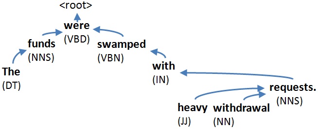
Dependency parsing of a sentence is one form of grammatical-reasoning of text. Given a sentence the goal is to output a directed-tree over the words, where an edge from one word to another indicate a dependency relation between the words. The output of dependency parsing is more complex than of shallow-parsing, in which the output is a sequence of grammatical roles per sentence, and is similar to the output defined by a context-free grammar. Concretely, given a sentence of length the goal is to connect each word to some other word or a special word called root, that is the labels are the words of that input sentence or the root. In other words, all words depended exactly in some other words (called head), yet an head may have many dependents. Exactly one word must depend in the root, and all other words depend on it directly of indirectly. As our goal is to construct a parse tree over sentences there is one global constraint: the graph induced must by acyclic with no loops. That is, a word can not be dependent of another word, which in turn is a dependent of the first word, or a word the is a dependent of it (directly or indirectly). Formally a parse tree for a sentence with words is a relation , where the special index indicates the root of the tree. For each word the set is of size (a function). The set is of size , as only a single word is connected to the root. Finally, the induced graphs has no loops.
An illustration of a dependency parse is shown in Fig. 1 .
We use a unified notation for both sequential labeling and dependency parsing (as well as other problems) and define a scoring function which assign a real scalar value scoring how well the complex label should be the label of the input . Given such a function a prediction is defined to be the labeling with maximal score, that is,
| (1) |
where are all possible labelings of the input , e.g. all possible parse trees for a given sentence .
In this work, we restrict ourself to linear functions of some parameters [Collins,2002, Crammer, Dredze, and Kulesza,2009], that is,
| (2) |
where is a joint feature mapping of an instance and a labeling into a common vector space. Features are derived from combinations of words (unigrams or n-grams), part-of-speech, orthographic features such as capital letters, hyphens and so on. The vector parameterize the function , where is chosen by a learning algorithm such that for all sentences in the training set, the label output by the system is close or similar to the correct label (or gold label) of these sentences, that is
| (3) |
should be close to the best label.
A brute-force approach for computing the best label is not feasible as, typically, the size of the set grows very fast with the size of the input . For example, in sequence labeling there are possible labeling of a sentence of length , and there are directed acyclic trees over words (or nodes).
We thus employ common approach and factor the scoring function by factoring the appropriate feature function . For sequence labeling we allow only functions over a single label or pairs of consecutive labels,
| (4) |
Such factorization allows to perform the search for the best labeling time linear in and quadratic in using the Viterbi dynamic-programming algorithm.

For dependency parsing we build on MSTParser of [McDonald et al.,2005] and focus on non-projective parsing (tree edges may cross) with non-typed (unlabeled) edges. MSTParser factors the score for each parse to be a sum of the score over its edges, that is,
where as mentioned above every pair represents a single edge between word and word . Example features are the distance between the two words, words identity and words part-of-speech. Using this factorization, the search for the best tree can be computed efficiently by first constructing a full directed graph over the words of the sentence with weighted edges and then outputting the maximal spanning tree (MST) of the graph, which can be computed for dense graphs in quadratic time in the length of the sentence using Chu-Liu-Edmonds (CLE) algorithm [Chu and Liu,1965, Edmonds, J.,1967, Tarjan, R. E.,1977].
3 Confidence Estimation
Many large-margin-based training algorithms maintain and output linear models in the form of Eq. (3). Linear models are easy to train, yet in the end-of-the-day such models are designed merely to make a prediction which is a single labeling given an input , with no additional information about the quality or correctness of that prediction. This behavior assumes that the predicted labeling will be used ignoring the quality of each specific output (as opposed to global quality of the system, such as average accuracy, precision or recall).
| Margin | Marginal | K-Best | K-Alternatives | |
| Based | Probability | Alternatives | by Stochastic | |
| Models | ||||
| Absolute | No | Yes | Yes | Yes |
| confidence score | (only relative) | |||
| Hyper-parameters | ||||
| tuning | No | Yes | Yes | Yes |
| Complexity | ||||
| Sequences | ||||
| Complexity | ||||
| Parsing | - |
There are situations for which additional information per labeling is useful, for example when the user of the prediction system has the option to ignore , or when using erroneous is worse than not using it at all. One possible scenario is when the output is used as an input of another system that integrates various input sources or is sensitive to the correctness of the specific prediction. In such cases, additional confidence information about the correctness of these feeds for specific input can be used to improve the total output quality. For example, data mining systems use NER predictors as sub-components. Such systems may use few NER predictors which all provide confidence information about their output, and allow the data-mining system to integrate better the output from all NER predictors, and overcome possible mistakes.
Another case where confidence information is useful, is when there is an additional agent that validates the output (as was done in building RCV1 [Lewis et al.,2004]). Confidence information associated with output can be used to direct the agent to small subset of “suspect” outputs rather than use a random sample or evaluate all outputs.
We now describe three methods to compute confidence in prediction of the form of a single number per prediction. One method only provide relative confidence information. This numeric information can be only used to compare two outputs and decide which is of better quality. One use of such relative confidence information is to rank all predictions or outputs according to their confidence numeric-score, and validate the output of the outputs which are assigned with the most low-confident score values. One property of this relative score is that any monotonic transformation of the confidence values yields equivalent confidence information (and ranking).
Other two methods described below provide absolute numeric confidence information in the prediction. Conceptually, the numeric confidence information is given as the probability of a prediction to be correct. We interpret these probabilistic outputs in a frequentists approach. A large set of events (predictions) all assigned with similar probability confidence value of being correct, indeed should contain about fraction of the predictions of that group correct. Clearly, any absolute information is relative as well, as two absolute confidence values may also be compared to each other to determine which output is of better quality.
In Sec. 3.1 we describe our relative confidence method which is based on extending the notion of margin originally used to design support-vector machines in the context of binary-classification [Boser, Guyon, and Vapnik,1992, Bartlett et al.,2000]. Intuitively, we define the confidence in a prediction to be the difference between the score of the (best) labeling , and an additional prediction.
Next, in Sec. 3.2 we define a probability distribution by using the score values as arguments of a suitable-function yielding non-negative values which sum to unit, and then compute the marginals induced from this distribution. Such method is used for example in conditional-random fields (CRF) [Lafferty, McCallum, and Pereira,2001b].
Finally, our third approach, which output absolute confidence information as well, is described in Sec. 3.3. This method generates few alternative outputs additional to , and evaluates the confidence by computing the agreement between the output and the alternatives. We use two methods to generate the alternatives: one deterministic based on extension of the prediction algorithms to produce -best predictions, and one stochastic based on sampling models. A comparison of the confidence estimation methods properties is summarized in Table 1 , each row is described in details in the appropriate place below.
3.1 A Margin-Based Method

Our first method extends the notion of margin known mainly in the context of support vector machines [Bartlett et al.,2000]. Originally, margin is a geometrical concept and is defined to be the distance of an input point embedded in some vector space to the separating hyperplane. Later (e.g. [Bredensteiner and Bennet,1999, Crammer and Singer,2001, Har-Peled, Roth, and Zimak,2002, Weston and Watkins,1999, Taskar, Guestrin, and Koller,2003]) it was extended in the context of multiclass problems. For example, in sequential labeling it is defined to be the difference between the best scoring labeling and the second best,
This definition is too crude for our purpose as we need a measure of confidence per unit, or word in our tasks. Thus, we refine the above definition and define the margin of the p word to be the difference in the score of the best labeling score and the score of the best labeling where we set the label of that word to anything but the label with the highest score. Formally, as before we define the best labeling , then the margin of the p word is defined to be,
| (5) |
where is the labeling of the p word according to the labeling of the entire input. Since labeling of consecutive words are dependent according to the model the labeling of additional words may change from by the restriction that the labeling of the p word is not its labeling according to the best labeling . In parsing, for example, changing the parent of a single word in a parse tree may cause a loop in the graph that require changing the parents of additional words to resolve the loop.
We refer to this method as Delta where the confidence information is the margin which is a difference or delta between two score values. Clearly, the absolute margin value provides confidence score that is only relative and not absolute, namely it can be used to compare the confidence in two labeling, yet there is no semantics defined over the scores as it is not calibrated to be in .
An illustration of the margin method is given in Fig. 2 for the sentence fragment Mr Smith founder of Smith Inc.. The top row of both panels shows the highest scoring labeling which attains a score of in our case. The second row of each panel shows the best labeling where the label of some word is restricted. The top panel shows the best labeling where the label of the word founder is restricted not to be N - its labeling according to . Clearly its score of is not higher than the score of the best labeling, as the operator is performed over a strict subset of possible labelings . The bottom panel shows similar process for the word of where its labeling is restricted from being N, and the one that has the highest score is Misc, the difference in score is which is defined to be the confidence value. Thus, in our example, the confidence in the labeling of the word of is higher than the confidence in the labeling of the word founder.
A straightforward implementation of the Delta method requires repeating the inference process times, once per word of the input, each time with a single constraint over the labeling, that is, the label is not allowed for the p word - the word for which the confidence is being evaluated. Such implementation costs . We used this approach for dependency parsing task, and thus the computation complexity is which is cubic in .
For the sequence labeling task the computation of Delta confidence can be improved by using the forward-backward-Viterbi algorithm (similar to standard forward-backward algorithm [Rabiner,1989]). This dynamic programming algorithm allows to efficiently compute the score of the best sequence labeling that includes a specific label constraint, therefore the computation of the Delta confidence scores can performed in , the same complexity as the standard Viterbi algorithm used for sequence labeling prediction.
3.2 Marginal-Probability Method
The second method we describe is based on specific function converting score values into probabilities.We follow the same modeling of conditional random fields (CRF) [Lafferty, McCallum, and Pereira,2001b] and define the conditional probability,
| (6) |
where is a normalization factor over all possible labeling to the input ,
| (7) |
and is a scaling parameter. While in some learning algorithms, such as CRFs, the model parameters are trained to maximize the log-likelihood of data using the above conditional probability, this is not the case for other algorithms such as ones that are based on large-margin such as the passive-aggressive [Crammer et al.,2006] algorithm or the confidence-weighted algorithm [Dredze, Crammer, and Pereira,2008, Crammer, Dredze, and Pereira,2008], both described below. For this reason the coefficient is used to allow tuning of the model score to confidence score.
We define the confidence in a prediction of the p word to be the marginal probability of that prediction, that is,
Using the dynamic-programming forward-backward algorithm [Rabiner,1989] for sequence labeling the marginal probability can be efficiently computed in for all assigned labels and . It is common to refer to the quantities computed by the forward-backward algorithm by , so we also refer to this method as Gamma. We report the results of this method only in the context of sequence labeling and not dependency parsing, as we found empirically that it is was shown not to perform well compared to Delta described above and some of the methods we describe next.
An illustration of this process appear in Fig. 3 where the best labeling appears in the top row, and the marginals for two words appear in the following rows. In this example the confidence in the prediction of the word founder is defined to be and the confidence in the prediction for the word of is defined to be , the marginal value in both cases. One notable property is that the confidence values are close to , this is because of the exponent-function used to convert scores to probabilities, a phenomena that was shown to appear in other contexts [Malkin and Bilmes,2009].
3.3 Confidence by Alternatives

This method works in two stages. First, a set of alternative labeling for a given input sentence are generated, where the predicted labeling is not necessarily one of the labeling. Then, the confidence in the predicted labeling is computed by evaluating the agreement (or disagreement) between and the alternatives. In other words, the confidence in the prediction for a specific word is defined to be the proportion of labeling which are consistent with the predicted label. Formally, let for be the labeling for some input , and let be the actual prediction for the input. (We do not assume that for some ). The confidence in the label of word is defined to be
| (8) |
The process is illustrated in Fig. 4. The input is given in the top row and the prediction is given in the next row. The example output includes a person name Mr Smith and a company name Smith Inc. In the next five rows there are five alternative labelings to the input sentence. Numeric confidence scores are given in the bottom line, and are the fraction of alternatives which agree with the labeling of the output. For example, in the alternative just after the output only the word Mr is part of the person name while the following word Smith is labeled as a none entity. The confidence for the word founder is as in three alternatives out of five the labeling of it (None) agrees with the labeling of the output. The confidence for the word of is as all alternatives agree with the labeling of the output (None).
We tried two major approaches to generate possible alternatives: deterministic and stochastic.
3.3.1 K-Best Predictions
The inference procedures are returning the labeling that achieves the highest score in Eq. (1), . We modify the inference algorithm to return not a single labeling but the best distinct labelings with highest score. Formally, we pick the top- distinct labelings that satisfy,
By definition we have that the first labeling is the predicted output and that all labelings differ from each other for . Specifically, we use the k-best Viterbi algorithm [Chow and Schwartz,1989] to find the k-best sequence labeling in , and for dependency parsing we used the k-best Maximum Spanning Trees algorithm [Hall,2007, Camerini, Fratta, and Maffioli,1980] to produce the parse trees with the highest score in .
We use two variants of this approach. The first variant assigns uniform importance to each of the labelings ignoring the actual score values. We call this method KB, for -best. The second variant assigns a specific importance weight to each labeling , and evaluate confidence using the weights, where we set the weights to be their score value clipped at zero from below . (In practice, top scores were always positive.) We call this method WKB for weighted -best. Eq. (8) is naturally extended to a weighted set,
| (9) |
3.3.2 Stochastic Models
Previous method used a single model to generate few alternatives. This approach is complimentary, we use a single model to generate (stochastically) few additional models, each is used to generate a single alternative (best according to itself) labeling. Concretely, given a model learned by some algorithm we induce a probability distribution over weight-vectors given , denoted by . We then draw a set of weight-vectors , and use each to output a best labeling according to it to get a set of alternatives,
| (10) |
Again we use two variants of this approach. The first variant is more generic we define the probability distribution over weights to be Gaussian with an isotropic covariance matrix, for some positive scale information , that is we have that, where are the parameters returned by the learning algorithm. The value of was tuned on the training set. We denote this method KD-Fix for -draws with fixed standard deviation. This method is especially appealing, since it can be used in combination with training algorithms that do not maintain confidence information, such as the Perceptron or PA.
The second variant is used with classifiers that not only maintain a single weight vector but also a distribution weight vectors. For example, the confidence weighted classifier (CW) described below in Sec. 4 maintains by definition a Gaussian distribution over weights, . We proceed as the previous variant, given an input the algorithm draws alternative weight vectors according the distribution maintained by CW scaled by scalar , that is , and output the best labeling with respect to each weight vector. Again the value of was tuned on the training set. We denote this method KD-PC for -draws by parameter confidence.
We stress that the two variants generating the set of alternatives are inherently different from each other. The first deterministic approach generates few labelings from the same model, all of the labelings are different from each other, and one of them is always the prediction . Additionally, although different from each other the labelings are close (or similar) to each other (in term of Hamming difference), as all attain very close (to the best) score values, because the score over sequences decompose to scores over words and pairs of adjacent words. The second stochastic approach generates one alternative per sampled model. With high probability these models differ from the model used to make the prediction, and thus the output labeling may be different from each of the alternatives. However, if the covariance matrix is close to zero, the sampled weight-vectors are likely to be close (in terms of Euclidean distance) to and thus produce similar labeling to , that is, there may be overlap between alternative labeling.
Using the stochastic models approach the alternative predictions are generated by executing the inference algorithm times, each time with different sampled model, therefore the computing complexity is , that is for parsing and for sequence labeling.
4 Learning
The algorithms described above to compute confidence are designed for linear models decomposed over units, and work with any algorithm in such setting. We evaluate the confidence estimation methods described in Sec. 3 using online learning algorithms [Cesa-Bianchi and Lugosi,2006]. These algorithms are fast, efficient, simple to implement and work well in practice. The passive-aggressive (PA) algorithms [Crammer et al.,2006] were shown to achieve state-of-the-art performance in many tasks such as NP chunking [Shimizu and Haas,2006], dependency parsing [McDonald, Crammer, and Pereira,2005b], learning preferences [Wick et al.,2009] and text segmentation [McDonald, Crammer, and Pereira,2005a]. Recently, confidence weighted (CW) algorithms were introduced for binary classification [Dredze, Crammer, and Pereira,2008, Crammer, Dredze, and Pereira,2008] and multi-class problems [Crammer, Dredze, and Kulesza,2009] and were shown to outperform many competitors. We next describe both PA and CW algorithms for structured prediction. Both versions are reductions from structured problems to binary classification in a manner similar to the reduction performed for parsing using the Perceptron algorithm [Collins,2002].
Online algorithms work in rounds. On the i round the online algorithm receives an input and applies its current rule to make a prediction , it then receives the correct label and suffers a loss . At this point, the algorithm updates its prediction rule with the pair and proceeds to the next round. A summary of online algorithms can be found in the book written by [Cesa-Bianchi and Lugosi,2006]. As noted above, in structured prediction we assume a joint feature representation, for (see Eq. (2) and the text after it).
Input:
- •
Joint feature mapping
- •
Tradeoff parameter
Initialize:
- •
For
- •
Get input
- •
Predict best labeling
- •
Get correct labeling
- •
Define
- •
Compute (from Eq. (12))
- •
Set
Output: Weight vector
Passive-Aggressive Learning
We first review a version of the passive-aggressive (PA) algorithms for structured prediction [Crammer et al.,2006, Sec. 10]. The algorithm maintains a weight vector and updates it on each round using the current input and label , by optimizing:
| s.t. | (11) |
where the loss is taken as the Hamming distance between the two labeling which is number of incorrect edges in the parse tree or incorrect labels in the sequence labeling tasks, and controls the tradeoff between optimizing the current loss and being close to the old weight vector. To solve Eq. (11) we define the difference between the feature vector associated with the true labeling and the feature vector associated with some labeling to be, and in particular, when we use the current model’s prediction we get,
The update of Eq. (11) can be computed analytically to get a structured version of PA-I :
| (12) |
The algorithm is summarized in Alg. 1. The theoretical properties of this algorithm were analyzed by [Crammer et al.,2006], and it was demonstrated on a variety of tasks (e.g. [Chechik et al.,2009]).
Confidence-Weighted Learning
Online confidence-weighted (CW) learning [Dredze, Crammer, and Pereira,2008, Crammer, Dredze, and Pereira,2008] generalizes the passive-aggressive (PA) update principle to multivariate Gaussian distributions over the weight vectors - . Originally, it was designed for binary classification and later was extended to multi-class problems [Crammer, Dredze, and Kulesza,2009], speech recognition [Crammer,2010] and sequence prediction [Mejer and Crammer,2010]. We now sketch a generalization for structured problems which contains all previous versions as special cases.
The mean contains the current estimate for the best weight vector, whereas the diagonal Gaussian covariance matrix captures the confidence in this estimate. More precisely, the diagonal elements capture the confidence in the value of the corresponding weight ; the smaller the value of is, the more confident is the model in the value of . Full matrices are not feasible as the dimension is in the order of millions.
CW classifiers are trained according to a PA rule that is modified to track differences in Gaussian distributions. At each round, the new mean and covariance of the weight vector distribution is chosen to be the solution of the following optimization problem,
| (13) |
where is the cumulative function of the normal distribution and controls the tradeoff between adjusting the model according to last example and being close to the old weight vector distribution. The larger the loss is, the larger probability we require for the event .
The solution for the CW updates is of the form,
| (14) |
where return a diagonal matrix which equals to the diagonal elements of the matrix . The two scalars and are computed using the mean and variance of the margin,
| (15) |
and are,
| (16) |
The method presented here is called 1-best binary reduction since the binary example for the update step at each round was generated as the difference between a single prediction, the model’s best prediction, and the true labeling. There are variants of this method that at each round utilize multiple predictions, usually the n-best predictions, to generate multiple binary examples for updating the model. Please see [Crammer, Mcdonald, and Pereira,2005, McDonald, Crammer, and Pereira,2005b] for more details.
Finally, we used parameter averaging with both algorithms. That is, during test time we are not using the final parameter vector , but instead using its average . It was shown to improve performance in other settings, and for us it either improved performance a bit, or did not make it worse.
5 Data
| Dataset | Sentences | Words | Features |
|---|---|---|---|
| NP chunking | 11.0 K | 259.0 K | 1.35 M |
| NER English | 17.5 K | 250.0 K | 1.76 M |
| NER Spanish | 10.2 K | 317.6 K | 1.85 M |
| NER Dutch | 21.0 K | 271.5 K | 1.76 M |
| Dataset | Sentences | Words | Features |
|---|---|---|---|
| Arabic | 1.5 K | 54.3 K | 1.03 M |
| Bulgarian | 12.8 K | 190.2 K | 2.64 M |
| Chinese | 56.0 K | 337.1 K | 4.92 M |
| Czech | 72.7 K | 1,249.0 K | 12.69 M |
| Danish | 5.2 K | 94.3 K | 1.22 M |
| Dutch | 13.3 K | 195.0 K | 2.36 M |
| English | 39.8 K | 950.0 K | 7.00 M |
| German | 39.2 K | 699.6 K | 6.99 M |
| Japanese | 17.4 K | 151.4 K | 0.85 M |
| Portuguese | 9.0 K | 206.6 K | 2.50 M |
| Slovene | 1.5 K | 28.7 K | 0.55 M |
| Spanish | 3.3 K | 89.3 K | 1.40 M |
| Swedish | 11.0 K | 191.4 K | 2.50 M |
| Turkish | 5.0 K | 57.5 K | 1.10 M |
We evaluated our algorithms on two types of structured predictions problems: sequence labeling and dependency parsing. For the sequence labeling experiments we used four large sequential classification datasets taken from the CoNLL-2000, 2002 and 2003 shared tasks: noun-phrase (NP) chunking [Kim, Buchholz, and Sang,2000], and named-entity recognition (NER) in Spanish, Dutch [Tjong and Sang,2002] and English [Tjong, Sang, and Meulder,2003]. The properties of the four datasets are summarized in Table 2 For the task of NP chunking we used the BIO system of labeling marking the first word (beginning) of a phrase (B), additional words of a phrase (in a phrase; I) and other words (O). For NER problems we used the same system for the four categories ending up with nine possible labels. Eight labels are the beginning of a name-entity (B) or being in it (I) for every the four categories: Location, Organization, Person and Miscellaneous. The ninth label is marking O(ther) words.
We followed previous feature generation process [Sha and Pereira,2003]. For NP chunking we used word and part-of-speech over a window of size (5) centered at the word to be labeled. For NER we used word and standard sub-word features including word, part-of-speech, suffix and prefix identity as well as standard orthographic features (e.g. word is capitalized), with all features over a window of size five (5) centered around the word at investigation.
To evaluate the task of dependency parsing we used datasets: languages used in CoNLL 2006 shared task (Arabic, Bulgarian, Chinese, Czech, Danish, Dutch, German, Japanese, Portuguese, Slovene, Spanish, Swedish and Turkish 11 1 See http://nextens.uvt.nl/~conll/ for details, and the English Penn Treebank. The properties of the datasets are summarized in Table 3 The feature representation of edges between words is generated as a combination of the connected words, the part-of-speech of the words and their local context, that is words before, after and between the connected words, the direction of the dependency (left or right) and the distance between the words (for more details see [McDonald, Crammer, and Pereira,2005b]). For dependency parsing evaluation we used a single split of training, development and testing sets for each language. The number of sentences in the training datasets is ranging between , with an average of sentences, words and features. The test sets contain sentences and words for all datasets, except English with sentences and words.
| CW | 5-best PA | Perceptron | |
|---|---|---|---|
| NP chunking | 0.947 | 0.946 | **0.944 |
| NER English | 0.877 | * 0.870 | * 0.862 |
| NER Dutch | 0.787 | 0.784 | * 0.761 |
| NER Spanish | 0.774 | 0.773 | * 0.756 |
6 Prediction Performance Evaluation
Our primary goal is developing new methods to estimate confidence in prediction, not prediction perse. Yet prediction itself is the end goal of learning. Furthermore, we could not find published performance evaluation of CW on structured prediction tasks, and the results below are among such first results. We thus briefly report for completeness the performance of CW comparing it with previous state-of-the-art online algorithms. Below we report in details the results of our evaluation of various confidence estimation algorithms. Our goal was to evaluate whether CW improves performance for these structured prediction tasks as it does for binary classification [Dredze, Crammer, and Pereira,2008, Crammer, Dredze, and Pereira,2008] and multiclass prediction [Crammer, Dredze, and Kulesza,2009]. As our goal is confidence and not achieving the best accuracy we note that the performance results we report now are not necessarily the best published in the literature as they are obtained by using existing tools, and specifically MSTParser ”out of the box” not incorporating recent parsing advancements.
We compared the performance of CW Alg. 2 with the passive-aggressive algorithm, which was shown to be a state-of-the art in both tasks. Specifically, we used -best PA (the value of five was shown to be optimal for various tasks [Crammer, Mcdonald, and Pereira,2005]) for sequence labeling and -best PA which is the training algorithm MSTParser uses for non-projective parsing [McDonald et al.,2005]. Additionally, we include the performance of the Averaged-Perceptron algorithm on the sequence prediction tasks to show various properties of all algorithms. It is omitted for parsing as it was shown to be inferior to PA [McDonald et al.,2005]. We ran CW with a diagonal covariance matrix, as full matrix is not feasible. Specifically, we used the update rule for full matrices and then removed the off-diagonal elements22 2 This was shown to perform the best compared with two other alternatives: update a full inverse and remove its off-diagonal elements, and compute an exact update for a diagonal covariance matrix.. We used parameter averaging with all methods, including CW, as it improved performance for all algorithms, especially on parsing.
We used 10-fold cross validation for sequence labeling and existing split of data into training, development and test set for parsing. Hyper-parameters ( for CW, for PA) were tuned for each sequence prediction task using a single run over a random split of the data into a three-fourths training set and a one-fourth test set and using a development set with sentences per language for parsing. All algorithms were executed for ten (10) iterations over the training set.
6.1 Sequence Labeling Performance Evaluation
The F-measure of all algorithms after 10 iterations is summarized in Table 4. In all four datasets CW algorithm outperforms PA that outperforms the Perceptron algorithm. The difference between CW and the Perceptron is statistically significant using paired t-test over the 10 folds, and between CW and PA it is significant in one dataset.
We further investigate the convergence properties of the algorithms in Fig. 5 in which we plot the recall and precision evaluated after each training round averaged across the folds. Each panel summarizes the results for a single dataset, and in each panel a single set of connected points corresponds to one algorithm. Points in the left-bottom of the plot correspond to early iterations and points in the right-top correspond to later iterations. Long segments indicate a big improvement in performance between two consecutive iterations.
High (in the y-axis) values indicate better precision and right (in the x-axis) values indicate better recall. The performance of all algorithms is converging in about iterations as indicated by the fact the points in the top-right of the plot are close to each other. The long segments in the bottom-left for the Perceptron algorithm indicate that this algorithm benefits more from more than one pass compared with the other algorithms. Interestingly, in NER Dutch and NER Spanish (two bottom panels), PA achieves slightly better recall than CW but is paying in terms of precision and overall F-measure performance.
6.2 Dependency Parsing Performance Evaluation
| Edge Accuracy | Complete Trees | |||
| Dataset | CW | 1-best PA | CW | 1-best PA |
| Arabic | 0.777 | 0.772 | 0.110 | 0.123 |
| Bulgarian | 0.899 | 0.898 | 0.410 | 0.397 |
| Chinese | 0.901 | 0.900 | 0.739 | 0.737 |
| Czech | 0.845 | 0.844 | 0.340 | 0.323 |
| Danish | 0.878 | 0.871 | 0.326 | 0.304 |
| Dutch | 0.830 | 0.831 | 0.282 | 0.282 |
| English | 0.888 | 0.889 | 0.292 | 0.287 |
| German | 0.886 | 0.888 | 0.412 | 0.409 |
| Japanese | 0.936 | 0.940 | 0.769 | 0.779 |
| Portuguese | 0.863 | 0.863 | 0.302 | 0.302 |
| Slovene | 0.782 | 0.777 | 0.266 | 0.256 |
| Spanish | 0.820 | 0.813 | 0.189 | 0.180 |
| Swedish | 0.865 | 0.866 | 0.404 | 0.391 |
| Turkish | 0.781 | 0.776 | 0.281 | 0.276 |
| Average | 0.854 | 0.852 | 0.366 | 0.360 |
Predicted edges accuracy of PA and CW are summarized in Table 5. The accuracy ranges from on Arabic to on Japanese, with an average of . Training the parser with CW algorithm compared to PA yield a small accuracy improvement in 8 of 14 languages, with maximal improvement of for Danish and Spanish and maximal degradation of for Japanese. The accuracy averaged over all the languages using CW is compared to achieved by PA. The percentage of , that is sentences where the parse tree was completely correct, was also improved by CW compared to PA in of languages, and averaged over all the languages the parser trained with CW got complete trees compared to .
We investigate the convergence results of the two algorithm in Fig. 6 where we plot the accuracy results (averaged over all the language) evaluated using the test set after each training iteration. After a single pass over the training data CW algorithm performs better than PA, achieving higher accuracy on 11 of 14 datasets and average accuracy of compared to . With additional passes over training data the performance gap is reduced, until finally after ten iteration PA closes most of the gap and achieves average accuracy lower than CW by only .
To conclude, in all tasks of sequence labeling and most tasks of dependency parsing, CW slightly improves over PA; which is also reflected in its averaged performance which is slightly better than the averaged performance of PA. Additionally, CW obtain high-performance after a single round, and benefit less from multiple iterations over data, as opposed to both PA and the Perceptron algorithm. This relation are consistent with previous evaluation of CW on both binary classification [Dredze, Crammer, and Pereira,2008, Crammer, Dredze, and Pereira,2008], multi-class prediction [Crammer, Dredze, and Kulesza,2009] and phoneme-recognition [Crammer,2010]. Yet, in all these previous work the improvement of CW over both PA and Perceptron was higher than the improvement we found here for sequence labeling and parsing. Currently, it is not clear why CW improves more over PA in the context of multi-class and binary prediction, and less in the context of structured prediction. One possible explanation is that implicitly CW exploits feature statistics. In the former simple problems the features are orthogonal per class, while in structured prediction, the features are sum over parts (as in Eq. (4)) and thus may have different statistical properties, such as dependencies.
7 Confidence Estimation Methods Evaluation
We now report an evaluation of the confidence estimation methods mentioned above. We trained a classifier using the CW algorithm running for ten (10) iterations on the training set and applied it to the testing set to obtain an initial labeling, the hype-parameter was set to its optimal value obtained in the experiments reported in Sec. 6. We then applied each of the confidence estimation methods on all the testing set labels. For sequences, a single split of four-fifths of the data was used as training set and the remaining one-fifth as testing set. For parsing we used the given split of the data into a training set and a test set as described above. For sequences, the fraction of words for which the trained model made a mistake ranges between (for NER Dutch) to (for NER Spanish). While for parsing the fraction of incorrect edges is between (for Arabic) to (for Japanese), with an average of .
Six algorithms and one baseline were evaluated. The baseline is random confidence scores for all the labels. The margin based method called Delta described in Sec. 3.1. The marginal based method called Gamma described in Sec. 3.2, and four methods based on alternatives described in Sec. 3.3. Two of these methods are based on top-K best prediction defined in Sec. 3.3.1, one using the output of the prediction algorithm as is called KB (-best) defined in Eq. (8), and the other is based on weighting its output called WKB (weighted -best) defined in Eq. (9). The other two alternatives-based methods are using stochastic models both described in Sec. 3.3.2. The first by inducing a Gaussian distribution over weights with covariance called KD-Fix for draws with fixed covariance, and the second by using the scaled covariance matrix learned by CW called KD-PC for -draws by parameter confidence.
For the KD-PC algorithm we note that the predictions of the CW algorithm are based solely on the mean weight vector and are invariant to initial scale of the covariance (as was noted elsewhere [Crammer, Dredze, and Pereira,2008]). Nevertheless, for the purpose of confidence estimation the scale of the covariance has a huge impact. Small eigenvalue of yield that all the samples of in Eq. (10) will be the same, while large values yield almost complete random vectors, ignoring the mean.
One possible simple option is to run CW few times with few possible initializations of the covariance and choose one copy based on the confidence evaluated on the training set. However, since the actual predictions of all these versions is the same and all the resulting covariance matrices will be proportional to each other [Crammer, Dredze, and Pereira,2008, Lemma 3] in practice we run the algorithm only once initializing the covariance with . Then, after training is completed, we pick the best covariance matrix of the form for a positive scalar where is the covariance output with initialization , and choose the best value using the training set.
The parameters of the confidence estimation methods: size of of the number of labelings used in the four first methods (KD-PC, KD-Fix, KB, WKB), the weighting scalar used in KD-PC and KD-Fix, and the coefficient of the Gamma method were tuned for each dataset on a development set according to the best measured average precision achieved in the task of incorrect prediction detection, described in Sec. 7.1.
We tried values in the range to for the parameter . For the number of labeling the values in were used. For the K-Draws methods, larger generally improved performance up to about with flat performance beyond that, so was set for all datasets (see also Sec. 7.3). The K-Best and WK-Best methods are more sensitive to value of and values between to were used across the different datasets. Performance degraded significantly for larger values of . For the parameter of Gamma method values between to were tried.
We evaluate the algorithms in two aspects of confidence: relative confidence (Sec. 7.1) and absolute confidence (Sec. 7.2) and two application: precision-recall tradeoff (Sec. 8.1) and active learning (Sec. 8.2).
7.1 Relative Confidence
In this experiment confidence estimation methods are evaluated in accordance to their ability to rank all the words in the test set (per dataset) having words for which there is a prediction mistake in the top and the correct predictions in the bottom. Conceptually, this task can be thought of as a retrieval task of the erroneous words. All words were ranked from low to high according to the confidence score in the prediction associated with each word by the various confidence methods. Then their performance in the task was evaluated in a few ways. We split the results according to the task type.
7.1.1 Sequence Labeling
The average precision for ranking the words of the test-set according the confidence in the prediction for the seven methods in sequence labeling is summarized in the left panel of Fig. 7 when training with CW. The algorithms are ordered from left-to-right: KD-Fix, KD-PC, Delta, Gamma, WKB, KB and random ordering. The average precision is computed by averaging the individual precision values computed at all ranks of erroneous words.
From the plot we observe that when having a random ordering the average precision is about the frequency of erroneous word, and clearly random ordering achieves the lowest (worst) average precision. The next two best methods are these based on K-Best predictions , where the weighted approach WKB outperforms the non-weighted version KB. Thus, using the actual score value into consideration improves the ability to detect erroneous words. Next in performance are Gamma and Delta, the margin-based and marginal-probabilities methods that outperform the K-best methods in all four datasets. Delta is better than Gamma in two of the dataset and equal in the other two. The two best performing methods are KD-Fix and KD-PC, where the former is better in three out of four datasets. The relative success of KD-Fix compared to KD-PC is surprising, as KD-Fix does not take into consideration the actual uncertainty in the parameters learned by CW, and in fact replaces it with a fixed value across all features.
Except for KD-PC that takes the parameter confidence information into consideration, all the other confidence estimation methods do not assume a confidence-based learning approach. We thus repeated the experiment using the passive-aggressive algorithm (PA) rather than CW for training the model. The results appear in the right panel of Fig. 7 and basically tell the same story: KD-Fix outperforms the margin-based and marginal-probabilities methods Delta and Gamma, and the K-Best Viterbi based methods, KB and WKB achieve lowest performance with the weighted version better than the non-weighted. Note that in general CW is slightly better than PA in the prediction task (Sec. 6) and thus retrieval of erroneous words on the set labeled by the PA model is slightly an easier task, this may explain some of the bars in the right panel are higher than their corresponding bars in the left panel.
Average precision does not tell the whole story - it encapsulates the detection of all the incorrect edges into a single number. More refined analysis is described via precision-recall (PR) plots showing the precision as more incorrect labels are detected. PR plots for model trained with CW algorithm are shown in Fig. 8. The plots for KD-PC and KB are omitted for clarity, KD-PC curve is very similar to KD-Fix and KB is worse than all the rest. The plots present the incorrect-labels detection precision in different recall values from to . We observe that the advantage of the K-Draws methods over other methods is consistent throughout the entire retrieval process. Interestingly, for low recall values of around , in NER in Dutch and Spanish, WKB performed better than Delta and Gamma, yet its performance quickly degraded for higher recall values.
To illustrate the effectiveness of the incorrect labels detection process Table 6 presents the number of incorrect labels detected vs. number of labels inspected for English NER dataset. The test set for this task includes words and the classifier made mistake on only words, that is, accuracy of . We show the number of incorrect labels detected after inspecting , and labels which are and of all labels. When using random inspection, the number of incorrect labels detected is, as expected, and of all mislabeled words. Yet when inspecting the labels according to the ranking induced by KD-Fix method, and of all mislabeled words were detected for the same effort.
| Words inspected | KD-Fix | Delta | Random |
|---|---|---|---|
| (% of total) | |||
| 500 (1%) | 336 (20%) | 278 (17%) | 15 (0.9%) |
| 2,500 (5%) | 1,148 (70%) | 1,003 (61%) | 83 (5%) |
| 5,000 (10%) | 1,415 (86%) | 1,310 (79%) | 164 (9.9%) |
7.1.2 Dependency Parsing
We applied the same methodology for evaluating the confidence estimation methods in the task of dependency parsing. Here, all predicted edges were ranked according to their confidence score ordered from low to high, and ideally, erroneous edges by the parser are ranked at the top. A summary of the average precision, computed at all ranks of erroneous edges, evaluated for all confidence estimation methods and all the datasets is summarized in Table 7.
The average precision achieved by random ordering is lower than all the methods and is about equal to the error rate for each dataset. Next are the K-Best methods, where the weighted version performs better than the non-weighted version. The margin-based Delta method improves significantly over the the K-Best methods. Finally, KD-fix and KD-PC methods achieve the best performance with KD-Fix a little better than KD-PC, and both K-Draws methods outperform Delta method on average and in of datasets. These results are consistent with the results observed for sequence labeling.
The Precision-Recall (PR) plots for several datasets are shown in Fig. 9 and provide deeper insight of the mistakes detection precision as more incorrect-edges are detected. (KD-PC plots are very similar to KD-Fix and omitted for clarity.) We observe that in most datasets KD-Fix performs significantly better than Delta in the early detection stage (first of the incorrect edges), while Delta performs better in late detection stages - the last of the incorrect edges. The second and third rows of Table 8 summarizes the precision obtained by all methods after detecting only incorrect edges and after detecting of the incorrect edges, averaged over all the datasets. (The first row of Table 8 summarized the average-precision averaged over all languages, and is copied from the last row of Table 7 for easier reference.) For example, in three datasets (Czech, Slovene and Portuguese) of Fig. 9, we observe an advantage of KD-Fix for low recall and an advantage of Delta in high recall. This observation is consistent with most other dataset not shown in these plots. Yet, in few languages, Arabic for example, KD-Fix outperforms or equal to Delta along the entire range of recall values. This phenomena was not observed for sequence labeling tasks where we found the K-Draws method to outperform the other methods throughout the entire retrieval process.
This phenomena emerges from the different properties of the two algorithms. KD-Fix assigns at most distinct confidence values to each edge - the number of models that agreed on that particular edge. As is, there is no mechanism to break ties (in each of the levels) and thus edges that are assigned with the same confidence level are ordered randomly relative to each other. Furthermore, in most datasets large fraction of the edges, , are assigned to one of the top-three possible confidence scores (i.e. ). As a results, the precision performance of KD-Fix drops sharply for recall values of and above. This can be seen by the fast decrease of the line with circle markers in three of plots in Fig. 9, except Arabic. On the other hand, we hypothesize that the low precision values obtained by Delta at low recall values (diamond in Fig. 9) is because Delta takes into account only two parses, the margin between the highest scoring edge (the predicted edge) and the second best edge, ignoring information about additional edges with score close to the highest score. In contrast, KD-Fix integrates scores of parse tress. In other words, Delta is more sensitive to small perturbations of score values compared with KD-Fix.
Based on this observation we propose combining both KD-Fix and Delta. The new method sets the confidence score of an edge to be a weighted mean of the score values of KD-Fix and Delta, with weights a and 1-a, respectively, for a value of . If the confidence value of two edges according to KD-Fix is different, the contribution of the score outputted by Delta is negligible, and the final score is very close to the score of only KD-Fix. On the other hand, if the score of KD-Fix is the same, as happen for large recall values, then Delta breaks arbitrary ties. In other words, when ordering all edges according to the new method, we first order edges according to confidence score of KD-Fix, then a secondary order is employed according to the confidence values of Delta among edges assigned same confidence score by KD-Fix. Not surprisingly, we name this method KD-Fix+Delta.
This new method enjoys the good of the two methods. As the results show in Table 8 it achieves the highest average-precision averaged over the datasets. It improves average-precision over KD-Fix in of datasets and over Delta in all datasets. From the second and third row of Table 8, we see that it has Precision very close to KD-Fix for recall of ( vs. ), and very close to Delta for recall of ( vs. ). Moving to Fig. 9, we observe that the curve associated with the new method (red ticks) is in general as high as the curves associated with KD-Fix for low values of recall, and as high as the curves associated with Delta for large values of recall.
Finally, similar to sequence labeling task, in dependency parsing all confidence estimation methods, except for KD-PC, can be used with a model that does not maintain parameters confidence information. We repeated the experiment but now training a model with the passive-aggressive algorithm, rather than CW. The results appear in the fourth row of Table 8. The results based on PA are consistent with the results based on CW, KD-Fix outperforms the margin-based and the K-Best trees methods, and combining KD-Fix and Delta improves the performance.
| KD-Fix | KD-PC | Delta | WKB | KB | KD-Fix | Random | |
| + Delta | |||||||
| Arabic | 0.621 | 0.623 | 0.565 | 0.373 | 0.366 | 0.622 | 0.223 |
| Bulgarian | 0.491 | 0.466 | 0.463 | 0.257 | 0.238 | 0.494 | 0.102 |
| Chinese | 0.465 | 0.466 | 0.452 | 0.190 | 0.150 | 0.473 | 0.102 |
| Czech | 0.539 | 0.548 | 0.506 | 0.301 | 0.290 | 0.555 | 0.152 |
| Danish | 0.502 | 0.497 | 0.460 | 0.303 | 0.280 | 0.499 | 0.124 |
| Dutch | 0.534 | 0.536 | 0.527 | 0.370 | 0.358 | 0.544 | 0.167 |
| English | 0.489 | 0.459 | 0.477 | 0.291 | 0.278 | 0.496 | 0.112 |
| German | 0.426 | 0.418 | 0.469 | 0.254 | 0.232 | 0.472 | 0.114 |
| Japanese | 0.512 | 0.525 | 0.535 | 0.235 | 0.151 | 0.541 | 0.064 |
| Portuguese | 0.586 | 0.570 | 0.559 | 0.323 | 0.311 | 0.606 | 0.143 |
| Slovene | 0.561 | 0.573 | 0.555 | 0.345 | 0.332 | 0.581 | 0.218 |
| Spanish | 0.637 | 0.634 | 0.592 | 0.351 | 0.342 | 0.644 | 0.184 |
| Swedish | 0.528 | 0.533 | 0.496 | 0.289 | 0.273 | 0.527 | 0.137 |
| Turkish | 0.603 | 0.590 | 0.589 | 0.372 | 0.342 | 0.609 | 0.221 |
| Average | 0.535 | 0.531 | 0.518 | 0.304 | 0.282 | 0.547 | 0.147 |
| KD-Fix | KD-PC | Delta | WKB | KB | KD-Fix | Random | |
| + Delta | |||||||
| Avg-Prec | 0.535 | 0.531 | 0.518 | 0.304 | 0.282 | 0.547 | 0.147 |
| Prec @10% | 0.729 | 0.723 | 0.644 | 0.470 | 0.441 | 0.724 | 0.145 |
| Prec @90% | 0.270 | 0.279 | 0.351 | 0.157 | 0.151 | 0.348 | 0.147 |
| Avg-Prec (PA) | 0.539 | - | 0.513 | 0.305 | 0.278 | 0.548 | 0.149 |
7.2 Absolute Confidence
| KD-Fix | KD-PC | Gamma | WKB | Random | |
| NER English | 0.036 | 0.021 | 0.053 | 0.108 | 0.548 |
| NER Dutch | 0.049 | 0.024 | 0.046 | 0.104 | 0.559 |
| NER Spanish | 0.034 | 0.030 | 0.049 | 0.046 | 0.543 |
| NP Chunking | 0.022 | 0.020 | 0.019 | 0.056 | 0.557 |
| Average | 0.035 | 0.024 | 0.042 | 0.078 | 0.552 |
| KD-Fix | KD-PC | WKB | Random | |
| Arabic | 0.076 | 0.057 | 0.175 | 0.402 |
| Bulgarian | 0.037 | 0.223 | 0.093 | 0.492 |
| Chinese | 0.044 | 0.024 | 0.223 | 0.497 |
| Czech | 0.087 | 0.024 | 0.109 | 0.451 |
| Danish | 0.119 | 0.095 | 0.068 | 0.476 |
| Dutch | 0.098 | 0.105 | 0.094 | 0.441 |
| English | 0.041 | 0.144 | 0.059 | 0.483 |
| German | 0.090 | 0.094 | 0.102 | 0.481 |
| Japanese | 0.064 | 0.039 | 0.122 | 0.524 |
| Portuguese | 0.099 | 0.107 | 0.085 | 0.465 |
| Slovene | 0.156 | 0.137 | 0.151 | 0.404 |
| Spanish | 0.083 | 0.028 | 0.123 | 0.429 |
| Swedish | 0.023 | 0.031 | 0.114 | 0.465 |
| Turkish | 0.105 | 0.142 | 0.127 | 0.404 |
| Average | 0.080 | 0.089 | 0.117 | 0.458 |
A second aspect of confidence prediction is the individual confidence values outputted by the various methods, rather than only comparing pairs of values. As before, suitable confidence estimation methods were applied on the entire set of predicted labels 33 3 The output of the Delta method can not be interpreted on their own, only relatively. In the context of binary classification there are few methods to generate absolute confidence from relative one [Platt,1998] using a sigmoid function. Yet, it could not be tuned properly in our setting since we tuned all methods according to their performance in relative confidence scenario (average-precision for ranking), where all parameters of Platt’s method perform equally good. . For every dataset and every algorithm we grouped the words according to the value of their confidence. Specifically, we used twenty (20) bins dividing uniformly the confidence range into intervals of size . For each bin, we computed the fraction of words predicted correctly from the words assigned to that bin. Ultimately, the value of the computed frequency should be about the center value of the interval of the bin. Formally, bin indexed contains words with confidence value in the range for . Let be the center value of bin , that is . The frequency of correct words in bin , denoted by is the fraction of words with confidence that their assigned label is correct. Ultimately, these two values should be the same, , meaning that the confidence information is a good estimator of the frequency of correct predictions. Methods for which are too pessimistic, predicting too high frequency of erroneous predictions, while methods for which are too optimistic, predicting too low frequency of erroneous words.
The results for sequence labeling are summarized in Fig. 10 and for dependency parsing in Fig. 12. Each panel in each figure summarizes the results for a single task (or language in parsing), where the value of the center-of-bin is plotted vs. the frequency of correct prediction , connecting the points associated with a single algorithm. Best performance is obtained when the resulting line is close to the line . Four algorithms are shown: KD-Fix, KD-PC, Gamma and WK-Best. The results of the K-Best method were inferior to all other methods and omitted for clarity.
For sequence labeling we observe from the plots that WKB is too pessimistic as its corresponding line is above the line . Gamma method tracks the line pretty closely in NP-Chunking and NER-Spanish datasets but it is too optimistic in the other two with its corresponding line is below the line . The KD-Fix method is too pessimistic on NER-Dutch and too optimistic on NER-English. The best method is KD-PC which tracks the line pretty closely in all four datasets.
For dependency parsing, in most languages KD-Fix and KD-PC methods perform very similarly. The distribution of this qualitative behavior of the KD methods among the datasets is: too optimistic in datasets, too pessimistic in and close to the line in datasets. The confidence scores produced by the WKB method are in general worse than KD-Fix and are too pessimistic with the line above . In quite a few datasets we observe that WKB is too optimistic in some confidence range and too pessimistic in another range. In most plots both in Fig. 10 and in Fig. 12 the curves on the left (low bin-values) are far from the line and with more fluctuation compared with the right area curves. This is because the left (low confidence) bins are less populated and thus the estimates are noisier.
Fig. 11 shows the distribution of the words in the bins according to confidence scores assigned by KD-Fix method on the four sequence labeling datasets. Blue bars represent the distribution of all the labels in the bins as percentage of total number of labels, green and red bars represent the distribution of correct/incorrect labels as percentage of the correct/incorrect labels. We see that of the labels populate the highest confidence bin, another populate the second highest bin and the rest of the bins are lightly populated. Among the correct labels even higher percentage is concentrated at the highest confidence bin, while the incorrect labels are distributed more evenly over many of the lower confidence bins.
| KD-Fix | KD-PC | Gamma | WKB | Random | |
| Sequences CW | 0.035 | 0.024 | 0.042 | 0.078 | 0.552 |
| Sequences PA | 0.031 | - | 0.039 | 0.080 | 0.543 |
| Parsing CW | 0.080 | 0.089 | - | 0.117 | 0.458 |
| Parsing PA | 0.068 | - | - | 0.122 | 0.456 |
The predicted vs. actual accuracy plots do not reflect the fact that different bins are not populated uniformly . We thus compute for each method the root mean-square error (RMSE) in predicting the bin center value given by
where is the number of words in the j bin. The computed RMSE values are presented in Table 11 both sequence labeling and parsing averaged over datasets. We observed a similar trend to the one appeared in the bins plots. For sequences, when using CW for training (top row in Table 11) , WKB is the least-performing method (after Random), then Gamma and KD-Fix, where each was better than the other in two datasets, and on average KD-Fix achieved lower RMSE. KD-PC performed best where it achieved lowest RMSE in three of four datasets and on average. Similar results, obtained when training with PA, appear in the second row of the table. KD-Fix achieved lowest RMSE in three of four datasets and on average, and WKB performs worst.
For parsing Table 11 presents the RMSE results averaged over all languages, for parser trained with CW (third row) and with PA (fourth row). For CW, both K-Draws methods perform better than WK-Best. KD-Fix yield lower RMSE than KD-PC in seven of the languages and higher in the other seven, and on average KD-Fix performed better than KD-PC (Table 10 presents results for all languages). This is in oppose to the results observed for sequences where KD-PC performed better than KD-Fix in all four datasets. When using PA for training, we also see that KD-Fix performed better than WK-Best method.
To conclude, both KD-Fix and KD-PC outperform all other methods in both settings and most datasets. The former is slightly better than the later, except in absolute evaluation for sequence labeling.
7.3 Effect of value on K-Draws methods performance
One of the two parameters that need to be tuned for the K-Draws methods is , the number of alternative labeling. As discussed above, for each word in each sentence these methods eventually output a single value between zero and one, interpreted as the probability of the prediction being correct. Conceptually, for every word we associate a coin with probability . Our goal is to estimate these probabilities up to a satisfying level, denoted by . These methods are used to estimate the coin’s bias by sampling from it, as defined in Eq. (8), Applying the inequality of [Chernoff,1952] and of [Hoeffding,1963] we have,
| (17) |
Denote by the total number of words in the test set, using the union bound we have,
Let be some confidence level. Then upper bounding the right-hand-side of the last inequality with and solving for we get,
Note that if we set to be the length of a confidence bin, then by setting the value of to be above the lower bound, we bound the probability that a word will not fall in the correct bin, or one of its two closet neighbors.
Concretely, we used bins, thus we set . Additionally, we set , and (see Table 2 and Table 3) we get, .
This estimate is pessimistic in many aspects. First, it is based on the assumption that the estimates of are independent, yet this is clearly not the case since features that tie the prediction for few words are used. In the extreme case, where the prediction of all words in a sentence are completely tied (that is, knowing the labeling of one word, induces a deterministic labeling of all other words), then the number of all words should be replaced with the number of all sentences a typical value of about , which yields a value of .
The discussion above is pessimistic in another sense. It assumes we need that all estimates will be close to their correct values . However, we are often not interested in estimating the bias values per-se, but estimating confidence for a practical purpose. For example, in the task of incorrect prediction detection, a good separation between the labels with high and low values is sufficient and error on the absolute value is acceptable. Therefore we can take the actual value of into consideration. Using the inequality of [Bernshtein,1946] (see also [J.V.Uspensky,1937]) we have,
| (18) |
For values close to the error is small which allows effective detection of high confidence labels. Comparing the right-hand-side of the last equation to we solve for the error interval and get a dependent error interval
where . In other words, for each value we get a different error interval such that with probability greater than all estimates falls within the interval .
The left plot of Fig. 13 presents error intervals for all estimated using KD-Draws method with different number of samples with probability greater than . For values of far from the intervals are low, compared with values of close to . The right plot presents for each value of the interval where its estimate may fall with high-probability using (Blue) and (Red) for confidence level . The two horizontal lines mark (with high-probability) the lowest possible estimate for , the lower and upper lines for and respectively. We see that for words with may have their corresponding estimate greater than words with , while when using only words with may have the corresponding estimate greater than labels with . This means, for example, that if we are interested in words that their prediction is with high-confident, then when using and picking all words with with high probability we will pick only words with . As expected, greater values of yield better error estimates so the choice of should be guided by the application of the confidence scores and the sensitivity to the estimate accuracy. Additionally, we observed in Fig. 11 that most (more than ) words have estimates . So for most words the estimates is pretty close to the correct values, which will not affect much the average precision or f-measure.
Although theoretically about is expected to yield good results, still this value is large for reasonable purposes. We evaluated the affect of for various values of and empirically found that for our practical purposes relatively small values of are sufficient and increasing beyond these values does not improve performance. Indeed, as mentioned above, for the K-Draws methods we set the value of by picking a best value of on a development set evaluating average precision in the task of incorrect prediction detection. Eventually we set a single value of for all datasets. Indeed, this value is one order of magnitude smaller than the most optimistic estimate above. One explanation is that the bounds are worst-case in the sense that we assumed that the estimate will be smaller than for all words with high-confidence and larger than for all words with low-confidence. Yet, there is no reason that this will happen in practice for all such words, only for a small fraction of them, and thus smaller values of yield in practice accurate estimates.
Fig. 14 presents average precision results achieved on the test sets using the KD-Fix method with different values of from to for all sequence labeling tasks and several dependency parsing tasks (the rest of the languages follow the same trend and omitted from the plot for clarity). We observe that even with , only two samples per sentence, the average precision results are better than random ranking in all tasks. As is increased to the performance is greatly improved. For , despite the very large theoretical estimation error, the results are better than the K-best methods for all tasks and for the NER tasks even better than Gamma and Delta. As is further increased the results continue to improve, yet at a more moderate rate, until reaching maximal results at for most tasks and results remain steady for larger values of up to 80. These curves can be used to tradeoff performance (average precision) with time, as the time complexity of this method is linear in .
8 Applications
Additionally of confidence estimation being useful by itself in some contexts, it is also useful for solving other problems. The next two sections present two example applications built on top of the algorithms presented so far. The first application is using the confidence information to trade-off precision and recall. In Sec. 8.1 we describe a modification of an NER system, allowing it to label less words as named-entities, but ask that the labeling will be with high precision. The second application, presented in Sec. 8.2, is performing active leaning in the context of sequence labeling, using the confidence information as a tool to choose which sentences should be labeled by the annotator.
8.1 Precision-Recall Tradeoff

Labeling all words with a specific tag yields maximal recall for that tag, as all words occurrence of that tag are labeled correctly, yet with the price of low precision, as many words are tagged wrongly. On the other hand, not labeling even one word (or labeling all word with the special tag of no tag) yields maximal precision for all tags, as there is not even a single word that is labeled mistakenly by some tag, yet the precision is zero as none of the words that should be tagged are indeed tagged. Clearly, one can move from the second extreme to the first by labeling or tagging more and more words with some tag. In various information extraction systems it is desirable to have the ability to control the tradeoff between high precision or high recall. In some scenarios a user may prefer that the system may label fewer words with a tag (low recall) yet to have the labeled words be tagged correctly (high precision), and in another scenarios the opposite is preferred, that is, labeling more words with some tag, yet at the price of low precision.
We propose the ability to perform such a system based on the confidence information outputted by various algorithms. We demonstrate the system using the task of named entity recognition. First, a NER algorithm produces a labeling for a given sentence, and then a confidence algorithm is used to output additional confidence score for each label. The system uses a tradeoff parameter to shift between the two extremes of high-recall and high-precision. The label of all words labeled with some tag, such as Per or Loc that their confidence is below the threshold is replaced by the N label indicating that no tag is associated with that word. The larger the value of is, the tag of more words that were labeled as named entities will be modified to a no-tag and the recall would be reduced. The lower the value of is, the lower number of words for which their tag is modified, and the recall is higher. In the optimal case, with a perfect confidence estimation algorithm, only the tag of words labeled with incorrect tag would been changed, yielding higher precision with no decrease of recall. Fig. 15 illustrates such NER system. The words Morgan Stanley are first labeled as Person with low confidence score of , the word Google is labeled as Organization with high confidence score of and the rest of the words are labeled with confidence score as N indicating they are not part of named entity. In this example the tradeoff threshold is set to , so the labels of Morgan Stanley that have confidence score below the threshold are replaced by N while the label of Google is not replaced as it has confidence score above the threshold. In this example, indeed Morgan Stanley was incorrectly labeled as Person instead of Organization so the replacement operation improves the system’s precision.
The left column of Fig. 16 shows the NER precision, recall and f-measure as the confidence threshold value increases from to which causes increasingly more tags such as Per to be replaced to a non-tag N. Each plot presents two sets of curves when using the confidence scores output by the KD-Fix algorithm and Gamma algorithm. The performance of KD-PC plot is similar to that of KD-Fix and of WKB is worse. Thus, both methods omitted for clarity. Delta is omitted since its output is not in the desired range of absolute confidence prediction. The top, middle and bottom curves for each of the two algorithms are precision, f-measure and recall respectively.
For English we observe a similar trend for both algorithms. For confidence threshold lower than no labels are replaced and the precision and recall scores remains constant. For larger confidence threshold values the precision score increases as we expected, yet the recall score drops. This indicates that both correct and incorrect NE tags are being replaced with a non-tag N. For confidence threshold values between the f-measure score remains about constant while precision score increases from to and recall score drops from to . This is a successful trade-off between recall and precision for the optimal f-measure value. For larger confidence threshold values the precision score continues to increase up to , yet at the price of significant drop in the recall score to and the f-measure score drops as well.
For NER in Spanish, we observe that for confidence thresholds up to , both methods allow similar balanced precision recall tradeoff such that the f-measure score is steady. Yet, for threshold values greater than the tradeoff based on KD-Fix confidence scores improves precision at cost of decreased recall more aggressively compared to tradeoff based on Gamma. The maximal precision score achieved using KD-Fix is compared to only with Gamma. In Spanish NER we also observe that when using Gamma for confidence, the precision score starts to drop along with recall scores for threshold values greater than . This indicates that more correct NE tags are replaced with a no-tag N compared with incorrect NE tags, which clearly is undesirable. A similar behavior of more aggressive tradeoff between precision and recall for KD-Fix than for Gamma is observed for Dutch. Here, the maximal precision score achieved using KD-Fix is compared to only with Gamma. Determining which behavior is preferable, aggressive or passive tradeoff, is application specific, yet for any given precision score having higher recall score is clearly preferable. For NP-chunking we observed similar trend (plots omitted) yet as precision starts from very high score of the increase was less significant compared to the NER cases.
An alternative view of the same tradeoff is shown using the standard precision-recall curves in the plots in the right column of Fig. 16. Each of the plots shows the precision vs. recall for four confidence estimation methods algorithms: KD-Fix, KD-PC, Gamma and WKB, one plot for each dataset. The bottom-right point of each curve reflects the precision and recall before using our algorithms to filter or reduce tags. (In fact, all curves coincide at this point as the same model is used to make label or tag the test data.)
As the confidence threshold value increases precision score improves and recall score decreases, yet each method goes via different route of trading-off precision and recall. An optimal confidence estimation method distinguishes between correct and incorrect NE tags labels, and thus improves precision while maintaining a constant recall values. Such optimal behavior is reflected by a vertical curve at the right area of the plots.
For all datasets WKB confidence score yields poor performance where the precision gain is small compared to the loss in recall. Furthermore, at some point precision drops as well. Additionally, KD-Fix and to some extent KD-PC allow the system to achieve higher-values of precision (curve ends with high value). Gamma achieves similar or slightly better precision values for high-recall, yet is not able to improve precision compared with KD-Fix (NER English and NER Dutch), or even the precision drops together with recall (NER Spanish).
We experimented also in performing tradeoff in the opposite direction: trading precision for higher recall. We used similar approach as described above. For words labeled with a no-tag N and with confidence score lower than some threshold , we replaced the N with some tag, which had the second highest score value according to the prediction model. By construction, a tag of some NE (such as Per) will by chosen. This tradeoff task is harder than trading-off recall and precision as described above, as even if a word that is incorrectly labeled with a no-tag N is identified, still the algorithm is required to choose what tag should it be labeled with. We observed that our confidence estimation methods detect effectively incorrect no-tag labels N. Using KD-Fix method the average confidence score of all the words labeled incorrectly with a no-tag N is , and respectively in NER English, Spanish and Dutch. These values are low compared to the high average confidence scores of , and respectively, of all words assigned correctly with a no-tag N (Fig. 11 illustrates the low overlapping in the distribution of confidence scores between the correct and incorrect labels). Yet choosing the correct tag for a word is a hard task. Eventually recall values for all three languages improved at most by while precision score dropped by .
We therefore made the task easier by merging the four NE categories (Person, Location, Organization, Misc) to a single NE category. A word that is labeled with low confidence as no-tag N can now be tagged as NE without committing to a specific category. The results are presented in Fig. 17. We see that using a single NE category improves the base precision and recall scores in all three datasets, the f-measure scores for English, Spanish and Dutch improve from , , to , , respectively (these f-measure scores are close to the score achieved for NP chunking task which also has just a single tag category).
For English when using KD-Fix confidence scores to tradeoff we observe that for confidence threshold lower than no labels are replaced. Then for confidence threshold values between the f-measure score remains about constant (even slightly improves) while recall score increases from to and precision score drops from to . This is a balanced trade-off between recall and precision for the optimal f-measure value. For confidence threshold values greater than the recall score increases a little more almost to but the precision score drops to and the f-measure score drops as well. Using Gamma confidence score for this dataset allows similar improvement in recall, but the precision scores drops significantly even for low confidence threshold values and falls to . Similar quantitative behavior was observed both for NER in Spanish and Dutch.
The right column of Fig. 17 present the precision-recall curves using all the confidence estimation methods algorithms: KD-Fix, KD-PC, Gamma and WKB, one plot for each dataset. The top-left point of each curve reflects the precision and recall before labeling any low confidence no-tags words as NE. As the confidence threshold value increases recall score improves and precision score decreases.
For all datasets KD-Fix and KD-PC perform better than the other methods by maintaining higher precision score for the same recall scores, and in Spanish and Dutch datasets they also allow the system to achieve higher recall values. In English WKB allowed achieving the highest recall value yet at cost of very low precision.
Finally, we note that such an experiment is not relevant in the context of parsing, as each word is assigned to another word (with an edge), and the asymmetry in NER labels of having tags and no-tags does not exist.
8.2 Active Learning
| Dataset | Random | KD-Fix | Effort reduction |
|---|---|---|---|
| NER English | 38K | 25K | 34% |
| NER Spanish | 80K | 60K | 25% |
| NER Dutch | 35K | 23K | 34% |
| NP chunking | 62K | 43K | 30% |
In active learning, algorithms choose which example would be labeled and be included in the training set. The rational is that the algorithm would choose to label examples which their label contribute the most to the learning process. Other examples, often the easy ones, will not be chosen for labeling as they are not adding to the learning process.
In a typical active learning setting there exists a large set of unlabeled data and a small set of labeled data. Learning is performed in iterations. On each iteration the current set of labeled data used to build a model, which is then used to choose a subset of examples to be labeled from remaining unlabeled examples. Many active learning algorithms differ in the way this subset is chosen. We use the confidence estimation methods for this purpose.
The experimental protocol we used is as follows. The initial set of labeled examples contains annotated sentences, and the initial set of unlabeled examples contains sentences. Evaluation is performed using an additional test set of sentences. Learning is performed using CW and then the resulting model and the confidence methods are applied to the set of remaining unlabeled sentences, yielding a rank over these sentences. Indeed, in standard binary or even multiclass prediction, many active learning algorithms are making a prediction for each and every example that is not labeled yet. For sequence prediction problems, labeling sentences is time consuming. Thus, on each iteration the algorithm first selects random sentences and a prediction (and confidence estimation) is performed only to this set. The algorithm then picks the sentences with the least confident value, which are then annotated and accumulated to the set of labeled data examples. Every such iterations (that is adding sentences) the performance of the resulting model is evaluated using the evaluation set. The process is repeated until sentences are labeled.
The experiments reported above were focused in estimating confidence for individual words. If for example, the output is given to a human, it is realistic to ask the human to verify the tagging of individual words as indeed most words are labeled correctly by the model. When moving to active learning, the situation changes. Now, all the words in a sentence are not labeled, thus if a human is required to label a single word, she may need to label adjacent words as well, having additional effort. We thus focused in active learning in the sentence level rather than the word level. We defined the confidence in a prediction of a sentence to be the minimal confidence score over words in that sentence. Then the algorithm is ranking sentences according to their confidence, breaking ties by favoring short sentences (assuming short sentences contains a larger fraction of informative words to be labeled than long sentences).
We evaluated scoring sentences using the confidence score of few methods, KD-Fix, KD-PC, Delta and Gamma44 4 We [Mejer and Crammer,2010] used two additional methods before, yet their performance was lower or about the same, and thus we omit them here for clarity.. As a baseline we used random sentences selection.
The averaged cumulative f-measure vs. number of words labeled is presented in Fig. 18 (as above KD-PC curves are close to KD-Fix curves and omitted for clarity). Left panels summarizes the results for a short horizon (small number of total-words). In two datasets random selection has the lowest performance, while Gamma is worse in Spanish. There is not clear winner among the other methods: KD-Fix is the best for NP-Chunking while Gamma is best for Dutch. The right panels show the results for more than training words, in log scale. In this scale, random selection performs the worst in all cases, and then again all the other methods performs about the same, except NER English where Gamma achieves lower performance.
As the goal of active learning is reducing the annotation effort, we compare the number of words required to be annotated when applying the proposed selection method using KD-Fix in order to achieve the same performance level as by random picking of sentences. The results are summarized in Table 12 For NER English dataset only words are required to achieve the same level of performance obtained by training on random words - a effort reduction. Similarly for Spanish, Dutch and Chunking about words have to be annotated to achieve the same performance of random labeling, a effort reduction.
9 Related Work
Confidence estimation methods for structured predication in NLP were investigated in previously and applied to tasks such as POS tagging, information extraction, machine translation, and automatic speech recognition (ASR).
[Culotta and McCallum,2004] propose several methods for confidence estimation for single and multi-word fields, and for entire records in a CRF based information extraction system. They describe a constrained forward-backwards algorithm that defines confidence as the ratio of total probability of any labeling for a given sentence with the total probability given a labeling constraint which is taken as the extracted field. The constrained forward-backwards yields same confidence scores as Gamma a for single token yet when extended to multi-word field it performed better. Additionally, they used an external maximum entropy classifier to classify fields as correct or incorrect based of set of features describing the extracted fields. The resulting posterior probability of the ”correct” label is used as the confidence measure. This method performed equally to the constrained forward-backwards method. [Kristjansson et al.,2004] shows how to improve interactive information extraction system accuracy by high-lighting low confidence fields, computed using these confidence scores, for the user to inspect and correct.
[Scheffer, Decomain, and Wrobel,2001] estimate confidence of single token label in HMM based information extraction system by a method similar to the Delta method we use. The label confidence score is the difference in the marginal probabilities of the best and second best label to the token. They use the single token confidence score to rank the labels and use this ranking for active learning.
[Ma, Randolph, and Drish,2001] describe HMM based ASR system where word marginal score and difference in scores between the two best alternatives are used to compute per-word confidence measures, similar to Gamma and Delta methods we use. They train SVM based on these features for deciding which word candidates to reject.
[Ueffing and Ney,2007] propose several methods for word level confidence estimation for the task of machine translation based on K-best translations. These methods are similar to the weighted and non-weighted K-best methods (KB and WKB) we use. They show the utility of the confidence scores for detecting incorrect translated words and for re-scoring candidate translations among the K-best alternatives and show improvement in translation quality.
[Gandrabur, Foster, and Guy,2006] describe using a neural network as a dedicated confidence estimation layer and evaluate it for ASR and for machine translation tasks. Both the ASR and translation systems provide a probabilistic score to their outputs, yet the dedicated confidence estimation layer can combine features and account for addition information that is not available to the prediction system and thus provide more useful confidence scores. They show the advantage of using a dedicated layer in ASR for the single word level and in the concept-level (semantic phrases) by rejecting incorrect recognitions. In context of interactive machine translation system with sequences of 1-4 words they gain advantage by avoiding incorrect translation suggestions.
About a decade ago, [Argamon-Engelson and Dagan,1999] used committee voting to evaluate the uncertainty in an example in a HMM based POS tagger. The committee of HMM taggers are sampled from the trained model in a manner similar to KD-PC method we use. Each HMM parameter is independently sampled from normal distribution with mean value equal to the trained parameter value and with per-parameter standard deviation according to the number of examples the parameter value was estimated by and multiplied by a ”temperature” coefficient. The committee of taggers were then used to produce a set of POS predictions and the uncertainty in each label is computed according to the disagreement among the committee predictions regarding that label. They used the uncertainty measure for guiding sample selection (active learning) and show that indeed this method reduces the required labeling effort compared to random or entire corpus labeling. However they did not evaluate directly the relative or absolute per-label confidence score for purpose such as detecting incorrect labels.
Confidence estimation was used in various additional setting of NLP applications such as binary and multi-class classification. For example, [Delany et al.,2005] describe confidence estimation method in an email spam filtering system based on combination of k-Nearest Neighbors features such as agreement among the neighbors and distance to closest same and opposite prediction. [Platt,1998] describes how to fit a sigmoid function to compute class posterior probabilities, that can serve as confidence scores, from the non-calibrated output score provided by the SVM in text classification tasks. [Xu et al.,2002] use confidence estimation in a question answering system by mixture of few heuristic correctness indicators and show that these confidence scores are useful for selecting between alternative answer sources. [Bennett, Dumais, and Horvitz,2002] use confidence scores, referred to as reliability-indicators, for combining predictions of different types of document classifiers. They show that confidence scores allows better aggregation of the prediction votes compared to other alternatives.
Finally, there has been much work on active learning for NLP applications including structured prediction tasks. For example [Thompson, Califf, and Mooney,1999] use minimal confidence in the extraction rules of a rules-based information extraction system to select instances for annotation. [Shen et al.,2004] use minimal margin of SVM along with considerations of instances representativeness and diversity in a NER system, and [Baldridge and Osborne,2004] (see also [Osborne and Baldridge,2004]) apply active learning for parsers.
10 Summary and Conclusions
We have studied few methods to estimate the per-word confidence in structured predictions. These algorithms were evaluated both in a relative settings and in a absolute setting. We also used the confidence score of these methods in two applications: increasing precisions while decreasing recall, and active learning. All-in-all we found that the two methods using sampling alternative models KD-PC and KD-Fix yield the best results. The former is induced from the CW algorithms, while the later can be used with any linear model. Generally KD-Fix performed a little better except for sequential labeling in absolute setting where KD-PC was better.
These methods were also found useful in increasing precision vs recall in sequence labeling tasks. Additionally, we showed that when combining these methods with active learning, one can reduce annotating effort by at least compared to random sampling. Understanding the theoretical properties of the problem and our algorithms remains an open problem to be addressed in the future.
acknowledgments
This research was supported in part by the Israeli Science Foundation grant ISF-1567/10. Koby Crammer is a Horev Fellow, supported by the Taub Foundations.
References
- [Argamon-Engelson and Dagan,1999] Argamon-Engelson, Shlomo and Ido Dagan. 1999. Committee-based sample selection for probabilistic classifiers. Journal of Artificial Intelligence Research, 11:335–360.
- [Baldridge and Osborne,2004] Baldridge, J. and M. Osborne. 2004. Active learning and the total cost of annotation. In EMNLP.
- [Bartlett et al.,2000] Bartlett, P.J., B. Schölkopf, D. Schuurmans, and A. J Smola, editors. 2000. Advances in Large Margin Classifiers. MIT Press.
- [Bennett, Dumais, and Horvitz,2002] Bennett, Paul N., Susan T. Dumais, and Eric Horvitz. 2002. Probabilistic combination of text classifiers using reliability indicators: models and results. In Micheline Beaulieu, Ricardo Baeza-Yates, Sung Hyon Myaeng, and Kalervo Järvelin, editors, Proceedings of SIGIR-02, 25th ACM International Conference on Research and Development in Information Retrieval, pages 207–214, Tampere, FI. ACM Press, New York, US.
- [Bernshtein,1946] Bernshtein, S.N. 1946. Probability theory (Russian). Moscow-Leningrad.
- [Boser, Guyon, and Vapnik,1992] Boser, B. E., I. M. Guyon, and V. N. Vapnik. 1992. A training algorithm for optimal margin classifiers. In Proceedings of the Fifth Annual ACM Workshop on Computational Learning Theory, pages 144–152.
- [Bredensteiner and Bennet,1999] Bredensteiner, E. J. and K. P. Bennet. 1999. Multicategory classification by support vector machines. Computational Optimizations and Applications, 12:53–79.
- [Camerini, Fratta, and Maffioli,1980] Camerini, P. M., L. Fratta, and F. Maffioli. 1980. The best spanning arborescences of a network. Networks, 10(2):91–110.
- [Cesa-Bianchi and Lugosi,2006] Cesa-Bianchi, N. and G. Lugosi. 2006. Prediction, Learning, and Games. Cambridge University Press, New York, NY, USA.
- [Chechik et al.,2009] Chechik, G., V. Sharma, U. Shalit, and S. Bengio. 2009. An online algorithm for large scale image similarity learning. In NIPS.
- [Chernoff,1952] Chernoff, H. 1952. A measure of asymptotic efficiency for tests of a hypothesis based on a sum of observations. Ann. Math. Statist., 23:493–507.
- [Chow and Schwartz,1989] Chow, Yen-Lu and Richard Schwartz. 1989. The -best algorithm: an efficient search procedure for finding top sentence hypotheses. In Proc. DARPA Speech & Natural Language Worksh., pages 199–202.
- [Chu and Liu,1965] Chu, Y. J. and T. H. Liu. 1965. On the shortest arborescence of a directed graph. Sci. Sin., Ser. A, 14:1396–1400.
- [Collins,2002] Collins, M. 2002. Discriminative training methods for hidden markov models: Theory and experiments with perceptron algorithms. In EMNLP.
- [Crammer et al.,2006] Crammer, K., O. Dekel, J. Keshet, S. Shalev-Shwartz, and Y. Singer. 2006. Online passive-aggressive algorithms. JMLR, 7:551–585.
- [Crammer, Dredze, and Kulesza,2009] Crammer, K., M. Dredze, and A. Kulesza. 2009. Multi-class confidence weighted algorithms. In EMNLP.
- [Crammer, Dredze, and Pereira,2008] Crammer, K., M. Dredze, and F. Pereira. 2008. Exact confidence-weighted learning. In NIPS 22.
- [Crammer, Kulesza, and Dredze,2009] Crammer, K., A. Kulesza, and M. Dredze. 2009. Adaptive regularization of weighted vectors. In NIPS 23.
- [Crammer, Mcdonald, and Pereira,2005] Crammer, K., R. Mcdonald, and F. Pereira. 2005. Scalable large-margin online learning for structured classification. Tech. report, Dept. of CIS, U. of Penn.
- [Crammer and Singer,2001] Crammer, K. and Y. Singer. 2001. On the algorithmic implementation of multiclass kernel-based vector machines. Jornal of Machine Learning Research, 2:265–292.
- [Crammer,2010] Crammer, Koby. 2010. Efficient online learning with individual learning-rates for phoneme sequence recognition. In IEEE Int. Conf. on Acoustics, Speech, and Signal Processing (ICASSP).
- [Culotta and McCallum,2004] Culotta, A. and A. McCallum. 2004. Confidence estimation for information extraction. In HLT-NAACL, pages 109–112.
- [Delany et al.,2005] Delany, Sarah Jane, Padraig Cunningham, Dónal Doyle, and Anton Zamolotskikh. 2005. Generating estimates of classification confidence for a case-based spam filter. In Héctor Muñoz-Avila and Francesco Ricci, editors, ICCBR, volume 3620 of Lecture Notes in Computer Science, pages 177–190. Springer.
- [Dredze, Crammer, and Pereira,2008] Dredze, M., K. Crammer, and F. Pereira. 2008. Confidence-weighted linear classification. In ICML.
- [Edmonds, J.,1967] Edmonds, J. 1967. Optimum branchings. J. Res. Nat. Bur. Standards, B71:233–240.
- [Gandrabur, Foster, and Guy,2006] Gandrabur, Simona, George Foster, and Lapal Guy. 2006. Confidence estimation for nlp applications. ACM Trans. Speech Lang. Process., 3:1–29, October.
- [Hall,2007] Hall, Keith. 2007. k-best spanning tree parsing. In In Proceedings of the 45th Annual Meeting of the Association for Computational Linguistics.
- [Har-Peled, Roth, and Zimak,2002] Har-Peled, S., D. Roth, and D. Zimak. 2002. Constraint classification for multiclass classification and ranking. In Advances in Neural Information Processing Systems 15.
- [Hoeffding,1963] Hoeffding, W. 1963. Probability inequalities for sums of bounded random variables. Journal of the American Statistical Association, 58(301):13–30, March.
- [J.V.Uspensky,1937] J.V.Uspensky. 1937. Introduction to Mathematical Probability. McGraw-Hill Book Company.
- [Kim, Buchholz, and Sang,2000] Kim, E.F. Tjong, S. Buchholz, and K. Sang. 2000. Introduction to the conll-2000 shared task: Chunking.
- [Kristjansson et al.,2004] Kristjansson, T., A. Culotta, P. Viola, and A. McCallum. 2004. Interactive information extraction with constrained conditional random fields. In AAAI, pages 412–418.
- [Lafferty, McCallum, and Pereira,2001a] Lafferty, J., A. McCallum, and F. Pereira. 2001a. Conditional random fields: Probabilistic models for segmenting and labeling sequence data.
- [Lafferty, McCallum, and Pereira,2001b] Lafferty, John D., Andrew McCallum, and Fernando C. N. Pereira. 2001b. Conditional random fields: Probabilistic models for segmenting and labeling sequence data. In Proceedings of the Eighteenth International Conference on Machine Learning, ICML ’01, pages 282–289.
- [Lewis et al.,2004] Lewis, David D., Yiming Yang, Tony G. Rose, and Fan Li. 2004. Rcv1: A new benchmark collection for text categorization research. Journal of Machine Learning Research (JMLR), 5:361–397.
- [Ma, Randolph, and Drish,2001] Ma, Changxue, Mark A. Randolph, and Joe Drish. 2001. A support vector machines-based rejection technique for speech recognition. In Proceedings of ICASSP’01, pages 381–384.
- [Malkin and Bilmes,2009] Malkin, Jon and Jeff Bilmes. 2009. Multi-layer ratio semi-definite classifiers. In Proc. IEEE Intl. Conf. on Acoustics, Speech, and Signal Processing, Taipei, Taiwan.
- [McDonald, Crammer, and Pereira,2005a] McDonald, R.T., K. Crammer, and F. Pereira. 2005a. Flexible text segmentation with structured multilabel classification. In HLT/EMNLP.
- [McDonald, Crammer, and Pereira,2005b] McDonald, Ryan T., Koby Crammer, and Fernando C. N. Pereira. 2005b. Online large-margin training of dependency parsers. In ACL.
- [McDonald et al.,2005] McDonald, Ryan T., Fernando C. N. Pereira, Kiril Ribarov, and Jan Hajic. 2005. Non-projective dependency parsing using spanning tree algorithms. In HLT/EMNLP.
- [Mejer and Crammer,2010] Mejer, A. and K. Crammer. 2010. Confidence in structured-prediction using confidence-weighted models. In EMNLP.
- [Osborne and Baldridge,2004] Osborne, M. and J. Baldridge. 2004. Ensemble-based active learning for parse selection. In HLT-NAACL.
- [Platt,1998] Platt, J. C. 1998. Probabilistic outputs for support vector machines and comparisons to regularized likelihood methods. In P.J. Bartlett, B. Schölkopf, D. Schuurmans, and A. J Smola, editors, Advances in Large Margin Classifiers. MIT Press.
- [Rabiner,1989] Rabiner, Lawrence R. 1989. A tutorial on hidden markov models and selected applications in speech recognition. In Proceedings of the IEEE, pages 257–286.
- [Scheffer, Decomain, and Wrobel,2001] Scheffer, Tobias, Christian Decomain, and Stefan Wrobel. 2001. Active hidden markov models for information extraction. In IDA, pages 309–318, London, UK. Springer-Verlag.
- [Sha and Pereira,2003] Sha, Fei and Fernando Pereira. 2003. Shallow parsing with conditional random fields. In Proc. of HLT-NAACL, pages 213–220.
- [Shen et al.,2004] Shen, Dan, Jie Zhang, Jian Su, Guodong Zhou, and Chew Lim Tan. 2004. Multi-criteria-based active learning for named entity recognition. In ACL, pages 589–596.
- [Shimizu and Haas,2006] Shimizu, N. and A. Haas. 2006. Exact decoding for jointly labeling and chunking sequences. In COLING/ACL, pages 763–770.
- [Tarjan, R. E.,1977] Tarjan, R. E. 1977. Finding optimum branchings. Networks, 7:25–35.
- [Taskar, Guestrin, and Koller,2003] Taskar, B., C. Guestrin, and D. Koller. 2003. Max-margin markov networks. In nips.
- [Thompson, Califf, and Mooney,1999] Thompson, Cynthia A., Mary Elaine Califf, and Raymond J. Mooney. 1999. Active learning for natural language parsing and information extraction. In Proc. 16th International Conf. on Machine Learning, pages 406–414. Morgan Kaufmann, San Francisco, CA.
- [Tjong, Sang, and Meulder,2003] Tjong, E.F., K. Sang, and F. De Meulder. 2003. Introduction to the conll-2003 shared task: Language-independent named entity recognition. In CoNLL, pages 142–147.
- [Tjong and Sang,2002] Tjong, Erik F. and K. Sang. 2002. Introduction to the conll-2002 shared task: Language-independent named entity recognition. In CoNLL.
- [Ueffing and Ney,2007] Ueffing, Nicola and Hermann Ney. 2007. Word-level confidence estimation for machine translation. Comput. Linguist., 33(1):9–40.
- [Weston and Watkins,1999] Weston, J. and C. Watkins. 1999. Support vector machines for multi-class pattern recognition. In Proceedings of the Seventh European Symposium on Artificial Neural Networks, April.
- [Wick et al.,2009] Wick, M., K. Rohanimanesh, A. Culotta, and A. McCallum. 2009. Samplerank: Learning preferences from atomic gradients. In NIPS Workshop on Advances in Ranking.
- [Xu et al.,2002] Xu, Jinxi, Ana Licuanan, Jonathan May, Scott Miller, and Ralph M. Weischedel. 2002. TREC 2002 QA at BBN: Answer selection and confidence estimation. In TREC.