Wyner-Ziv Coding Based on Multidimensional Nested Lattices

For a set of $n$ linearly independent basis vectors $\{\mathbf{m}_{1},\mathbf{m}_{2},\ldots,\mathbf{m}_{n}\}$, an $n$-dimensional lattice $\Lambda$ is composed of all integral combinations of the basis vectors:

where $\mathbf{M}=[\mathbf{m}_{1},\mathbf{m}_{2},\ldots,\mathbf{m}_{n}]$ is the generator matrix and $\mathbb{Z}=\{0,\pm 1,\pm 2,\ldots\}$ is the set of integers. For a vector $\mathbf{x}=[x_{1},x_{2},\ldots,x_{n}]^{T}$, the nearest-neighbor quantizer associated with $\Lambda$ is $Q_{\Lambda}(\mathbf{x})=\arg\min_{\mathbf{l}\in\Lambda}||\mathbf{x}-\mathbf{l}||$. The basic Voronoi cell of $\Lambda$, defined by $\mathcal{V}=\{\mathbf{x}:Q_{\Lambda}(\mathbf{x})=\mathbf{0}\}$, specifies the nearest-neighbor decoding region. Important quantities for $\mathcal{V}$ include the cell volume $V=\int_{\mathcal{V}}d\mathbf{x}$, the second moment $\sigma^{2}=\frac{1}{nV}\int_{\mathcal{V}}||\mathbf{x}||^{2}d\mathbf{x}$ and the normalized second moment $G(\Lambda)=\sigma^{2}/V^{\frac{2}{n}}$. The minimum of $G(\Lambda)$ of all the $n$-dimensional lattices is denoted as $G_{n}$. From [13], $G_{n}\geq 1/2\pi e,\forall n$ and $\lim_{n\to\infty}G_{n}=1/2\pi e$.

Let $\Lambda_{F}$ be a fine lattice with a generator matrix $\mathbf{M}_{F}$. Similarly, let $\Lambda_{C}$ be a coarse lattice with a generator matrix $\mathbf{M}_{C}$. A pair of $n$-dimensional lattices $(\Lambda_{F},\Lambda_{C})$ is nested in the sense of $\Lambda_{C}\subset\Lambda_{F}$, if $\mathbf{M}_{C}=\mathbf{M}_{F}\cdot\mathbf{P}$, where $\mathbf{P}$ is an $n\times n$ integer matrix with determinant greater than one (in absolute value). We define the nesting ratio $N=V_{C}/V_{F}$, where $V_{F}$ and $V_{C}$ are the cell volumes of the fine and coarse lattice, respectively.

There is one special case where $\Lambda_{C}$ is geometrically similar to $\Lambda_{F}$, which means that $\Lambda_{C}$ can be obtained from $\Lambda_{F}$ by applying a similarity transform [8] including a rotation, change of scale and possibly a reflection. $\Lambda_{C}$ is strictly similar to $\Lambda_{F}$ when reflection is not used. We also refer to $\Lambda_{C}$ as a similar sublattice to $\Lambda_{F}$.

Throughout the paper, we follow the high-resolution assumption in [7], which means $V_{F}$ is sufficiently small such that the probability density function (pdf) of $Z$ is approximately constant over each Voronoi cell of the fine lattice $\Lambda_{F}$.

The encoding and decoding scheme is the same as in [7], which is simplified from [5] under the high-resolution assumption. The scheme is described as follows:

• •

  The encoder quantizes $\mathbf{x}$ to $\mathbf{x}_{Q_{\Lambda_{F}}}=Q_{\Lambda_{F}}(\mathbf{x})$, compute the coset leader $\mathbf{s}=\mathbf{x}_{Q_{\Lambda_{F}}}-Q_{\Lambda_{C}}(\mathbf{x}_{Q_{\Lambda_{F}}})$, and transmits the index corresponding to $\mathbf{s}$.

• •

  The decoder receives $\mathbf{s}$ and reconstructs $\mathbf{x}$ as $\widehat{\mathbf{x}}=\mathbf{s}+Q_{\Lambda_{C}}(\mathbf{y}-\mathbf{s})$.

Under this formulation, the rate per dimension is given by $R=\frac{1}{n}\log_{2}(\frac{V_{C}}{V_{F}})$. In our practical design, we also use minimum MSE estimation as described in [7].

The development of this paper is heavily based on the theta series. Given a lattice $\Lambda$, the theta series [13] is defined as

where $q=e^{j\pi\tau}$ ($\Im(\tau)>0$). Using the change of variable $j\tau\rightarrow\tau$ ($\tau>0$ real), it can alternatively be expressed as

Theta series of some standard lattices are given in [13]. In general, theta series are not easy to evaluate, and their derivatives are even more complex to calculate. Fortunately, there is a class of lattices for which the computation of such functions is tractable, the even unimodular lattices. A detailed description of such lattices can be found in [14].

A lattice $\Lambda$ is unimodular [13] if $\Lambda$ is integral, i.e., $\mathbf{M^{T}M}$ is an integer matrix, and $|\det\Lambda|=1$ or equavlently $\Lambda$ is equal to its dual $\Lambda^{*}$, i.e., $\Lambda=\Lambda^{*}$. If $\Lambda$ is integral, then $\|\mathbf{l}\|^{2}$ is necessarily an integer for all $\mathbf{l}\in\Lambda$. Further, if $\|\mathbf{l}\|^{2}$ is an even integer for all $\mathbf{l}\in\Lambda$, then $\Lambda$ is called an even unimodular lattice. Many exceptional lattices such as the Gosset lattice $E_{8}$ or the Leech lattice $\Lambda_{24}$ are even unimodular.

We introduce now the three Jacobi theta functions [13],

Now, consider the Eisenstein series,

where $\zeta\left(s\right)$ is the Riemann zeta function,

We can relate $E_{4}\left(q\right)$ and the Jacobi theta functions through the relation,

Another fundamental series is the so-called modular discriminant defined as,

which is also related to the three Jacobi theta functions through the identity

Remarkably, theta series of all even unimodular lattices can be expressed as polynomials in the two variables $E_{4}$ and $\Delta$:

We present an accurate calculation of the rate-distortion, based on the high-resolution assumption.

To compute (10), we need to enumeration all lattice points $\mathbf{l}_{C}\in\Lambda_{C}$, and those points $\mathbf{l}_{F}\in\mathcal{V}_{C}$. The latter may be done by checking all points $\mathbf{l}_{F}$ within the covering radius of $\Lambda_{C}$: $\mathbf{l}_{F}\in\mathcal{V}_{C}$ if and only if $\mathbf{l}_{F}$ is decoded to $0$ in $\Lambda_{C}$.

In Fig. 1, we give the rate-distortion performance of fine lattice $\mathbb{Z}^{8}$ and $E_{8}$. The sublattice is generated from the expand-rotate method described in the next Section. We also give the corresponding lower bound in [7] for comparison. From Fig. 1 we can see in dimension eight, the lower bound in [7] is tight for the best quantization lattice $E_{8}$ in this dimension, but has a gap to our theoretical calculation for the $\mathbb{Z}^{8}$ lattice. We find this is also true for other dimensions.

Albeit accurate under the high-resolution assumption, the method in the preceding subsection unfortunately does not lend much insight into the selection criterion of a good coarse lattice. Let us reexamine the $D_{C}$ component in (8)

which should be minimized. Of course, this problem itself is not tractable due to the integration over the basic Voronoi region.

To deal with this problem, the common approach is to choose a coarse lattice to maximize $P(\mathbf{z}\in\mathcal{V}_{C})$, which is reduced to the standard approach to channel coding. However, this standard approach does not quite capture the essence of Wyner-Ziv coding, since the metric in (12) is clearly different. Alternatively, one could derive either the upper or lower bound by using the covering or packing radius, the latter of which has already been done by Liu et al. [7]. Again, in addition to the computational complexity, it is not insightful.

Here, we propose a new upper bound using the the derivative of the theta series.

Now the problem reduces to that of finding a coarse lattice which maximizes the derivative of the theta series (note that its derivative is negative). We formalize this new criterion as the following Proposition:

As the theta series of even unimodular lattices are polynomial in $E_{4}$ and $\Delta$, it is enough to find the derivatives of these two series. The Ramanujan system [16] gives the answer. It expresses the derivatives of $E_{2}$, $E_{4}$ and $E_{6}$ as functions of themselves:

As we are interested in the functions $E_{k}\left(e^{-2\pi\tau}\right)$ for $k=4,6$, we get

and so, combining (6), (16) and (17), we obtain the derivative of the modular discriminant with respect to $\tau$:

This means that, using (7), (16) and (18), we are able to get the derivative of the theta series of an even unimodular lattice as a function of $E_{2}$, $E_{4}$ and $E_{6}$.

Recall that a clean similar sublattice means the boundary of its Voronoi cell does not touch any fine lattice points [8]. It is known that clean similar sublattices perform better than non-clean ones [7]. In this subsection we aim to find clean similar sublattices. A similar technique was used in solving multiple-description problem [17]. In a multiple-description framework proposed in [18], a number of clean similar sublattice constructions were given by extending the result in [8]. We will form our own constructions to be suitably used in nested lattices based on their constructions.

In the two-dimensional case, we introduce a complex-valued multiplying factor $\xi=a+bi$, $a,b\in\mathbb{Z}$, which is multiplied to the fine lattice points to obtain the coarse lattice points [18]. For various $\xi$, this calculation should generate both clean and non-clean similar sublattices. The clean similar sublattices were addressed in [18], where the authors proved the sublattice $\xi\mathbb{Z}^{2}$ is clean if and only if the nesting ratio $a^{2}+b^{2}$ is odd, and the sublattice $\xi A_{2}$ is clean if and only if $a$ and $b$ are relatively prime.

Next, we give the nested lattice construction based on $\mathbb{Z}^{4}$. We use the ring of Lipschitz integer quaternions $\mathbb{H}_{0}=\{a+bi+cj+dk,a,b,c,d\in\mathbb{Z}\}$, where $i$,$j$,$k$ are unit quaternions. Let an arbitrary point in a four-dimensional fine lattice $\Lambda_{F}$ be denoted as $\mathbf{l}_{F}=x+yi+zj+wk$. Then set the multiplying factor $\xi$ as $\xi=a+bi+cj+dk$. Multiplying $\xi$ with the fine lattice points $\mathbf{l}_{F}$ gives the coarse lattice points $\mathbf{l}_{C}$. The calculated $\mathbf{l}_{C}$ is equivalent to the product shown below:

So if the generator matrix of the fine lattice is the identity matrix, the first matrix above can be seen as the generator matrix of the coarse lattice.

More generally, it was shown in [18] that for lattices $\Lambda=\mathbb{Z}^{4l},l=1,2,3\dots$, if there exists a geometrically similar sublattice of nesting ratio $N$, then $N$ should be of the form $m^{n/2}$ for some integer $m$, where $n=4l$ is the dimension. From [18], the nesting ratio $N$ must be odd to make sure the similar sublattices are clean. From our simulation, the nesting ratios which are odd perfect squares indeed give better performance than others. The simulation results are shown in Fig. 3.

In this subsection, we present a more general method to obtain sublattices by scaling and rotation of the fine lattice. The obtained sublattices are not necessarily clean. We set a parameter, $\beta$, as the expanding factor. The way to generate the similar coarse lattice is as follows:

• •

  First expand the fine lattice by multiplying the expanding factor $\beta$, such that the lattice points with the smallest norm greater than zero in the fine lattice become the outermost points in the basic Voronoi cell of the coarse lattice. When $\beta$ is an integer, there is always a less (or equal) number of coarse lattice points on each shell (formed by points of equal norm) of the coarse lattice than in the fine lattice. This requirement can be fulfilled by using integer expanding factors.

• •

  For non-integer expanding factors, some expanded lattice points may not be a subset of the fine lattice. This case does not only happen to only one point, but also to a group of points with the same norm. The angle between these points and their fine lattice counterparts can be detected and calculated. Due to symmetry, these angles for points with the same norm are the same. So we can rotate the expanded lattice points by this angle, to match the positions of those fine lattice points. Also, the rotation for all the norms should be the same since the expanded lattice is similar to the fine one; so the rotated coarse lattice remains the similar shape as the original fine lattice.

The values of $\beta$ giving rise to sublattices are those norms of the fine lattices. So $\beta$ is not necessarily an integer. By exploiting tables of theta series in [13], we can find a sublattice.

Using this method, we now give the simulation results of the rate-distortion performance for nested lattice Wyner-Ziv coding for $D_{n}$, $E_{8}$ and $\Lambda_{24}$.

In the three-dimensional case, we implement the scheme using both $D_{3}$ and $D_{3}^{\ast}$. The rate-distortion performance is shown in Fig. 5. Compared to the one- and two-dimensional case, the three-dimensional scheme gives less distortion. Also notice NLC using $D_{3}^{\ast}$ is better than the one using $D_{3}$.

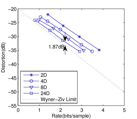
The simulation results using $D_{4}$ and $E_{8}$ are similar, and are both better than the three-dimensional case. At rate $1.5$ bits per sample, their distortion gaps to the Wyner-Ziv limit are $2.52$ dB and $1.07$ dB, respectively.

Moreover, for $\Lambda_{24}$, our scheme gives distortion performance closer to the Wyner-Ziv limit than the SWC-NQ scheme proposed in [7], especially at low rates. Results in [7] show a gap of distortion $1.53$ dB from the Wyner-Ziv limit while our gap is less than $1.28$ dB at rate less than three bits per sample for $\Lambda_{24}$. See Fig. 6.

One can also see that the “increasing gap” between the rate-distortion curve of NLC and the Wyner-Ziv limit [7] indeed exists in concrete implementation. Nonetheless, from Fig. 6, this widening gap as rate increases can be handled by increasing the dimension. In the meantime, the rate can not be too high in sensor network applications. So the gap is acceptable with $8$- or $24$-dimensional lattices. By increasing the dimension of NLC as the rate increases, a constant gap from the Wyner-Ziv limit can be maintained.

Code designs above are restricted to those proposed in [13]. Although they have acceptable performance and low complexity, it is better to have a scheme existing in any dimensions. Hence, we use the ensemble of good nested lattice codes proposed in [9] based on the concept of random lattices. The random lattice ensemble in [9] can be generated as follows.

• •

  Take $p$ to be prime.

• •

  Define a $k\times n$ generator matrix $M$, where $M_{i,j}$ is uniformly distributed on $(0,\dots,p-1),i=1,\dots,k;j=1,\dots,n$.

• •

  Apply Construction A in [9] to obtain the lattice $\Lambda_{F}^{\prime}$.

The $n$-dimensional cubic lattice $\mathbb{Z}^{n}$ can be viewed as a sublattice of the random lattice $\Lambda_{F}^{\prime}$ [9]. Hence, for any dimension, various nested lattices can be obtained by simply applying different linear transformations $\mathbf{G}$ to both $\mathbb{Z}^{n}$ and $\Lambda_{F}^{\prime}$. Obviously, the resultant sublattice is not necessarily similar. The nest ratio $N=p^{n-k}$.

To make the nested ensemble good for the Wyner-Ziv problem, the fine lattice should be good for source coding and the coarse lattice good for channel coding. This is proved in [19] by extending the results in [9]. Also, both the coarse lattice $\mathbf{G}\mathbb{Z}^{n}$ and the fine lattice $\mathbf{G}\Lambda_{F}^{\prime}$ should be good for quantization. To make $\mathbf{G}\mathbb{Z}^{n}$ good for quantization, $\mathbf{G}$ should be the generator matrix of a good quantizing lattice [13], e.g., the hexagonal lattice in dimension two and $E_{8}$ in dimension eight.

However, such lattices are not easy to decode. We use the sphere decoding algorithm described in [20] for the quantization to the random lattices, whose speed is tolerable if $n\leq 24$.

Examples for dimensions $2$, $4$, $8$ and $24$ are given in Fig. 7. The rate-distortion performance approaches the Wyner-Ziv limit as dimension increases and the gap is only $1.87$ dB within the limit for dimension twenty-four. The performance is very close to explicit lattices like the Leech lattice.

Since the elements of $\mathbf{M}$ are uniformly distributed over $\mathbb{Z}_{p}$ for large $p$ and since the decoding is not easy, this ensemble is of theoretic value only.

References

- [1] Z. Xiong, A. D. Liveris, and S. Cheng, “Distributed source coding for sensor networks,” IEEE Signal Processing Magazine, vol. 21, no. 5, pp. 80–94, 2004.
- [2] D. Slepian and J. Wolf, “Noiseless coding of correlated information sources,” IEEE Trans. Inform. Theory, vol. 19, no. 4, pp. 471–480, 1973.
- [3] A. Wyner and J. Ziv, “The rate-distortion function for source coding with side information at the decoder,” IEEE Trans. Inform. Theory, vol. 22, no. 1, pp. 1–10, 1976.
- [4] R. Zamir and S. Shamai, “Nested linear/lattice codes for Wyner-Ziv encoding,” Proc. Inform. Theory Workshop, Killarney, Ireland, pp. 92–93, June 1998.
- [5] R. Zamir, S. Shamai, and U. Erez, “Nested linear/lattice codes for structured multiterminal binning,” IEEE Trans. Inform. Theory, vol. 48, no. 6, pp. 1250–1276, 2002.
- [6] S. D. Servetto, “Lattice quantization with side information,” Proc. IEEE Data Compression Conference (DCC), 2000.
- [7] Z. Liu, S. Cheng, A. D. Liveris, and Z. Xiong, “Slepian-Wolf coded nested lattice quantization for Wyner-Ziv coding: High-rate performance analysis and code design,” IEEE Trans. Inform. Theory, vol. 52, pp. 4358–4379, 2006.
- [8] J. H. Conway, E. M. Rains, and N. J. A. Sloane, “On the existence of similar sublattices,” Canad. J. Math., vol. 51, pp. 1300–1306, 1999.
- [9] U. Erez and R. Zamir, “Achieving (1/2) log(1+SNR) on the AWGN channel with lattice encoding and decoding,” IEEE Trans. Inform. Theory, vol. 50, no. 10, pp. 2293–2314, 2004.
- [10] P. D. Fiore, “Scale-recursive lattice-based multiple-access symbol constellations,” IEEE Trans. Inform. Theory, vol. 56, no. 1, pp. 211–223, 2010.
- [11] M. Sartipi and F. Fekri, “Distributed source coding using short to moderate length rate-compatible LDPC codes: The entire Slepian-Wolf rate region,” IEEE Trans. Commun., vol. 56, no. 3, pp. 400–411, 2008.
- [12] Y. Yang, S. Cheung, Z. Xiong, and W. Zhao, “Wyner-Ziv coding based on TCQ and LDPC codes,” IEEE Trans. Commun., vol. 57, no. 2, pp. 376–387, 2009.
- [13] J. H. Conway and N. J. A. Sloane, Sphere Packings, Lattices and Groups. Springer-Verlag, 1998.
- [14] F. Oggier, P. Solé, and J.-C. Belfiore, “Lattice codes for the wiretap Gaussian channel: Construction and analysis,” Mar. 2011. [Online]. Available: http://arxiv.org/abs/1103.4086
- [15] W. Ebeling, Lattices and Codes. Vieweg, 1994.
- [16] S. Ramanujan, “On certain arithmetical functions,” Trans. Cambridge Philos. Soc., vol. 22, p. 159–184, 1916.
- [17] S. D. Servetto, V. A. Vaishampayan, and N. J. A. Sloane, “Multiple description lattice vector quantization,” Data Compression Conference, pp. 13–22, 1999.
- [18] S. N. Diggavi, N. J. A. Sloane, and V. A. Vaishampayan, “Asymmetric multiple description lattice vector quantizers,” IEEE Trans. Inform. Theory, vol. 48, no. 1, pp. 174–191, 2002.
- [19] D. Krithivasan and S. S. Pradhan, “Lattices for distributed source coding: Jointly Gaussian sources and reconstruction of a linear function,” IEEE Trans. Inform. Theory, vol. 55, no. 12, pp. 5628–5651, 2009.
- [20] C. P. Schnorr and M. Euchner, “Lattice basis reduction: Improved practical algorithms and solving subset sum problems,” Math. Program., vol. 66, pp. 181–191, 1994.