1Introduction

MPP-2011-62

Hard-Thermal-Loop Corrections in Leptogenesis II:
Solving the Boltzmann Equations

Clemens P. Kießig¹¹ 1 E-mail: ckiessig@mpp.mpg.de, Michael Plümacher²² 2 E-mail: pluemi@mpp.mpg.de

Max-Planck-Institut für Physik (Werner-Heisenberg-Institut),
Föhringer Ring 6, D-80805 München, Germany

Abstract

We investigate hard-thermal-loop (HTL) corrections to the final lepton asymmetry in leptogenesis. To this end we solve the Boltzmann equations with HTL-corrected rates and $C\!P$ asymmetries, which we calculated in paper I of this series. We pay special attention to the influence of the two leptonic quasiparticles that arise at non-zero temperature. We include only decays and inverse decays and allow for the lepton modes to be either decoupled from each other, or to be in chemical equilibrium by some strong interaction, simulating the interaction with gauge bosons. In two additional cases, we approximate the full HTL lepton propagators with zero-temperature propagators, where we replace the zero-temperature mass by the thermal mass of the leptons $m_{\ell}(T)$ or the asymptotic mass $\sqrt{2}\,m_{\ell}(T)$ . We compare the final lepton asymmetries of the four thermal cases and the zero-temperature case for zero, thermal and dominant initial neutrino abundance. The final lepton asymmetries of the thermal cases differ considerably from the vacuum case and from each other in the weak washout regime for zero initial neutrino abundance and in the intermediate regime for dominant initial neutrino abundance. In the strong washout regime, the final lepton asymmetry can be enhanced by a factor of two in the case of strongly interacting lepton modes.

1 Introduction

The question of the origin of all things was always essential to mankind and has driven them to search for answers in science, among others. Physics as the science of nature and within physics, cosmology as the science of the order and the evolution of the universe, address this question and have their own formulation of it. What is the origin of the matter that is the building block of all things we observe, including ourselves?

The matter in nature consists of leptons and the much heavier baryons, which are in turn made up of quarks. According to the standard model of particle physics (SM), matter particles, quarks or leptons, can only be created in pairs together with their antiparticles, that is, antiquarks and antileptons, at least in perturbation theory. If we assume that the early universe was indeed without form and void , that is in the language of particle physics, there was no excess of one particle species over the other, there would have to be an equal amount of particles and antiparticles today. More specifically, since annihilation of particles and antiparticles proceeds at fast rates, no structures like atoms, molecules, galaxies, stars, planets, DNA, cells and finally living organisms could have formed and we would observe a universe populated almost exclusively by photons and the slowly interacting neutrinos. This scenario is obviously not realised. If we believe in inflation, we cannot assume a sizeable matter-antimatter asymmetry as an initial condition of the universe because that asymmetry would be diluted by inflation, not even mentioning the highly unsatisfactory character of such an approach from a scientific point of view. Therefore we have to employ a baryogenesis theory, a mechanism that creates a baryon asymmetry dynamically and explains the value of

\displaystyle\eta\equiv\left.\frac{n_{B}-n_{\bar{B}}}{n_{\gamma}}\right|_{0}=(6.16\pm 0.16)\times 10^{-10}\,.

(1)

This value has been inferred from the WMAP seven-year cosmic microwave background (CMB) anisotropy data [1], where $n_{B}$ , $n_{\bar{B}}$ , and $n_{\gamma}$ are the number densities of baryons, antibaryons, and photons, respectively, and the subscript 0 implies present cosmic time. The value agrees with the abundance of light elements inferred from big bang nucleosynthesis.

Leptogenesis [2] is a very attractive baryogenesis theory, since it simultaneously explains the creation of the baryon asymmetry and the smallness of neutrino masses via the seesaw mechanism [3, 4, 5, 6, 7, 8]. We add three heavy right-handed neutrinos $N_{i}$ to the SM, which are assumed to have rather large Majorana masses $M_{i}$ , close to the scale of some possibly underlying grand unified theory (GUT) [9], $E_{\rm GUT}\sim 10^{15\ldots 16}\,{\rm GeV}$ . The interaction with the SM neutrinos suppresses their mass when we integrate out the heavy neutrinos. In the early universe, the heavy neutrinos decay into leptons and Higgs bosons and create a lepton asymmetry, which is lateron converted to a baryon asymmetry by the anomalous sphaleron processes [10, 11]. The three Sakharov conditions [12] that are necessary for a baryogenesis theory are fulfilled, that is lepton number $L$ and $B-L$ are violated, $C\!P$ symmetry is violated in the decays and the decays can be out of equilibrium.

Ever since the development of the theory 25 years ago, the calculations of leptogenesis dynamics have become more refined and many effects and scenarios that have initially been neglected have been considered³³ 3 For an excellent review of the development in this field, we refer to reference[13].. Notably the question how the hot and dense medium of SM particles influences leptogenesis dynamics has received increasing attention over the last years [14, 15, 16, 17, 18, 19, 20, 21]. At high temperature, particles show a different behaviour than in vacuum due to their interaction with the medium: they acquire thermal masses, modified dispersion relations and modified helicity properties. All these properties can be summed up by viewing the particles as thermal quasiparticles with different behaviour than their zero-temperature counterparts, much like the large zoo of single-particle and collective excitations that are known in high density situations in solid-state physics. At high temperature, notably fermions can in the hard-thermal-loop-limit (HTL) occur in two distinct states with a positive or negative ratio of helicity over chirality and different dispersion relations than at zero temperature, where these dispersion relations do not break the chiral symmetry as a zero-temperature mass does.

Thermal effects have been considered by references [14, 15, 16, 17, 18, 19, 20, 21]. Notably reference [15] performs an extensive analysis of the effects of thermal masses that arise by resumming propagators using the HTL resummation within thermal field theory (TFT). However, the authors approximated the two fermionic helicity modes with one simplified mode that behaves like a vacuum particle with its zero-temperature mass replaced by a thermal mass⁴⁴ 4 Moreover, an incorrect thermal factor for the ${C\!P}$ -asymmetry was obtained, as has been pointed out in reference [22].. Due to their chiral nature, there are serious consequences to assigning a chirality breaking mass to fermions, hence the effects of abandoning this property should be examined. Moreover, it seems questionable to completely neglect the negative-helicity fermionic state which, according to TFT, will be populated at high temperature. We argue in this study that one should include the effect of the fermionic quasiparticles in leptogenesis calculations and possibly in other early universe dynamics, since they behave differently from zero-temperature states with thermal masses, both conceptually and regarding their numerical influence on the final lepton asymmetry. We do this by analysing the dynamics of a leptogenesis toy model that includes only decays and inverse decays of neutrinos and Higgs bosons, but takes into account all HTL corrections to the leptons and Higgs bosons, paying special attention to the two fermionic quasiparticles. In a slightly different scenario, we assume chemical equilibrium among the two leptonic modes, thereby simulating a scenario where the modes interact very fast. As a comparison, we calculate the dynamics for two models where we approximate the lepton modes with ordinary zero-temperature states and modified masses, the thermal mass $m_{\ell}(T)$ and the asymptotic mass of the positive-helicity mode, $\sqrt{2}\,m_{\ell}(T)$ .

This paper is the second part of a two-paper series, where we have calculated the HTL-corrections to $C\!P$ -asymmetries in the first part [23]. The topic of this work is solving the Boltzmann equations with HTL-corrected rates and $C\!P$ -asymmetries. It is structured as follows: In section 2, we briefly review the imaginary time formalism of thermal field theory (TFT) and discuss the hard thermal loop (HTL) resummation. In section 3, we summarise and present our previous calculations of interaction rates and $C\!P$ -asymmetries in references[24], [25] and [23]. Section 4 deals with the evaluation of the Boltzmann equations. We derive the equations and compare our four thermal scenarios, wich are the decoupled and strongly coupled two-mode approach and the one-mode approach with thermal and asymptotic mass, to the vacuum case. We show the evolution of the abundances for three different initial conditions for the neutrinos, that is, zero, thermal and dominant abundance. We explain the dynamics of the different cases in detail and find considerable differences both of the thermal approaches to the vacuum case and of the two-mode cases to the one-mode cases. We summarise the main insights of this work in the conclusions and give an outlook on future work and prospects. In appendix B, we derive Boltzmann equations at zero temperature, while in appendix C, we explicitly perform the subtraction of on-shell propagators for our cases.

2 Propagators at Finite Temperature

When going to finite temperature [26], one has to employ ensemble weighted expectation values of operators rather than the vacuum expectation values, so for an operator $\hat{A}$ we get

\displaystyle\langle 0|\hat{A}|0\rangle\rightarrow\langle\hat{A}\rangle_{\rho}\equiv{\rm tr}(\rho\hat{A})\,.

(2)

There are two formalisms for calculating Green’s functions at finite temperature, the imaginary time formalism and the real time formalism. Both are equivalent and we employ the imaginary time formalism, where the $k_{0}$ -integration is replaced by a sum over discrete energies, the so-called Matsubara frequencies.

Naive perturbation theory at finite temperature can lead to serious conceptual problems, such as infrared divergent [27, 28] and gauge dependent [29, 30] results and results that are not complete to leading order. In order to cure these shortcomings, the hard thermal loop (HTL) resummation technique has been invented [31, 32]. One distinguishes between hard momenta of order $T$ and soft momenta of order $gT$ , where $g$ is the coupling constant of the corresponding theory. In a strict sense, this is only possible in the weak coupling limit where $g\ll 1$ . If all external momenta are soft, then the bare thermal propagators have to be replaced by resummed propagators. The self-energies that are resummed are the HTL self-energies, for which all internal momenta are hard. For a scalar field with a HTL-self-energy $\Pi$ , the resummed effective HTL-propagator $\Delta^{*}$ follows from the Dyson-Schwinger equation in figure 1 as

	$\displaystyle{\rm i}\,\Delta^{*}$	$\displaystyle={\rm i}\,\Delta+{\rm i}\,\Delta\left(-{\rm i}\,\Pi\right){\rm i}\,\Delta+\dots$
		$\displaystyle=\frac{{\rm i}}{\Delta^{-1}-\Pi}=\frac{{\rm i}}{K^{2}-m_{0}^{2}-\Pi}\,,$		(3)

where $\Delta$ is the bare propagator, $K$ the momentum and $m_{0}$ the zero-temperature mass of the scalar.

Refer to caption — Figure 1: The resummed scalar propagator.

The dispersion relation for this effective excitation is given by the pole of the propagator as

\displaystyle k_{0}^{2}=k^{2}+m_{0}^{2}+\Pi\,,

(4)

so we get an effective mass of $m_{\rm eff}^{2}=m_{0}^{2}+m_{S}^{2}$ where the thermal mass of the scalar is given by the self-energy, which is proportional to $gT$ , $m_{S}^{2}=\Pi\propto(gT)^{2}$ . It is possible to neglect the zero-temperature mass if $m_{S}\gg m_{0}$ .

For fermions with negligible zero-temperature mass, the general expression for the self-energy in the rest frame of the thermal bath is given by [33]

\displaystyle\Sigma(P)=-a(P)\not{P}-b(P)\not{u}\,,

(5)

where $u^{\alpha}=(1,0,0,0)$ is the four-velocity of the heat bath. The factors $a$ and $b$ are given by

	$\displaystyle a(P)$	$\displaystyle=\frac{1}{4p^{2}}\left[{\rm tr}\left(\not{P}\Sigma\right)-p_{0}{\rm tr}\left(\gamma_{0}\Sigma\right)\right]\,,$		(6)
	$\displaystyle b(P)$	$\displaystyle=\frac{1}{4p^{2}}\left[P^{2}{\rm tr}\left(\gamma_{0}\Sigma\right)-p_{0}{\rm tr}\left(\not{P}\Sigma\right)\right]\,.$

In the HTL limit, the traces are given by [26]

	$\displaystyle T_{1}\equiv{\rm tr}\left(\not{P}\Sigma\right)$	$\displaystyle=4\,m_{F}^{2}\,,$
	$\displaystyle T_{2}\equiv{\rm tr}\left(\gamma_{0}\Sigma\right)$	$\displaystyle=2\,m_{F}^{2}\frac{1}{p}\ln\frac{p_{0}+p+{\rm i}\,\epsilon}{p_{0}-p+{\rm i}\,\epsilon}\,,$		(7)

where the effective thermal fermion mass $m_{F}\propto gT$ depends on the interaction that gives rise to the fermion self-energy.

The resummed fermion propagator is then written as

\displaystyle S^{*}(K)=\frac{1}{\not{K}-\Sigma_{\rm HTL}(K)}\,.

(8)

It is convenient to rewrite this propagator in the helicity-eigenstate representation [34, 35],

\displaystyle S^{*}(K)=\frac{1}{2}\Delta_{+}(K)(\gamma_{0}-\hat{\bf k}\cdot\boldsymbol{\gamma})+\frac{1}{2}\Delta_{-}(K)(\gamma_{0}+\hat{\bf k}\cdot\boldsymbol{\gamma}),

(9)

where $\hat{\bf k}={\bf k}/k$ , and

\displaystyle\Delta_{\pm}(K)=\left[-k_{0}\pm k+\frac{m_{F}^{2}}{k}\left(\pm 1-\frac{\pm k_{0}-k}{2k}\ln\frac{k_{0}+k}{k_{0}-k}\right)\right]^{-1}\,.

(10)

This propagator has two poles, the zeros of the two denominators $\Delta_{\pm}$ . The poles can be seen as the dispersion relations of single-particle excitations of the fermions that interact with the hot plasma,

\displaystyle k_{0}=\omega_{\pm}(k)\,.

(11)

We have presented an analytical expression for the two dispersion relations making use of the Lambert $W$ function in reference [24]. The dispersion relations are shown in figure 2.

Note that even though the dispersion relations resemble the behaviour of massive particles and $\omega=m_{F}$ for zero momentum $k$ , the propagator $S^{*}(K)$ (9) does not break chiral invariance like a conventional mass term. Both the self energy $\Sigma(K)$ (5) and the propagator $S^{*}(K)$ anticommute with $\gamma_{5}$ . The Dirac spinors that are associated with the pole at $k_{0}=\omega_{+}$ are eigenstates of the operator $(\gamma_{0}-\hat{\bf k}\cdot\boldsymbol{\gamma})$ and they have a positive ratio of helicity over chirality, $\chi=+1$ . The spinors associated with $k_{0}=\omega_{-}$ , on the other hand, are eigenstates of $(\gamma_{0}+\hat{\bf k}\cdot\boldsymbol{\gamma})$ and have a negative helicity-over-chirality ratio, $\chi=-1$ . At zero temperature, fermions have $\chi=+1$ . The introduction of a thermal bath gives rise to fermionic modes which have $\chi=-1$ . These modes have been called plasminos since they are new fermionic excitations of the plasma and have first been noted in references [33, 36].

We can introduce a spectral representation for the two parts of the fermion propagator (10) [37],

\displaystyle\Delta_{\pm}(K)=\int_{-\infty}^{\infty}{\rm d}\omega\frac{\rho_{\pm}(\omega,k)}{\omega-k_{0}-{\rm i}\,\epsilon}\,,

(12)

where the spectral density $\rho_{\pm}(\omega,k)$ [34, 38] has two contributions, one from the poles,

\displaystyle\rho^{\rm pole}_{\pm}(\omega,k)=Z_{\pm}(\omega,k)\,\delta(\omega-\omega_{\pm}(k))+Z_{\mp}(\omega,k)\,\delta(\omega+\omega_{\mp}(k))\,,

(13)

and one discontinuous part,

\displaystyle\rho^{\rm disc}_{\pm}(\omega,k)=\frac{\frac{1}{2}\,m_{F}^{2}(k\mp\omega)}{\left\{k(\omega\mp k)-m_{F}^{2}\left[Q_{0}(x)\mp Q_{1}(x)\right]\right\}^{2}+\left[\frac{1}{2}\,\pi\,m_{F}^{2}(1\mp x)\right]^{2}}\times\theta(k^{2}-\omega^{2})\,,

(14)

where $x=\omega/k$ , $\theta(x)$ is the heaviside function and $Q_{0}$ and $Q_{1}$ are Legendre functions of the second kind,

\displaystyle Q_{0}(x)=\frac{1}{2}\ln\frac{x+1}{x-1}\,,\hskip 28.45274ptQ_{1}(x)=x\,Q_{0}(x)-1\,.

(15)

The residues of the quasi-particle poles are given by

\displaystyle Z_{\pm}(\omega,k)=\frac{\omega_{\pm}^{2}(k)-k^{2}}{2\,m_{F}^{2}}\,,\quad{\rm where}\quad Z_{+}+Z_{-}=1\,.

(16)

One can describe the non-standard dispersion relations $\omega_{\pm}$ by momentum-dependent effective masses $m_{\pm}(k)$ which are given by

\displaystyle m_{\pm}(k)=\sqrt{\omega_{\pm}^{2}(k)-k^{2}}=\sqrt{2\,Z(\omega,k)}\,m_{F}\,.

(17)

These masses are shown in figure 3.

Considering gauge theories, one might also have to use HTL-corrected effective vertices that are related to the propagators by Ward identities [26]. We do not consider these vertices since we are only looking at Yukawa vertices. In the HTL framework, it is sufficient to use bare propagators if at least one of the external legs is hard. However, it is always possible to resum self-energies and thus capture effects which arise from higher-order loop diagrams and take into account the appearance of thermal masses and modified dispersion relations in a medium. In fact, since the effective masses we encounter do typically not satisfy the condition $m_{\rm eff}\ll T$ but are rather in the range $m_{\rm eff}/T\sim 0.1$ – $1$ , the effect of resummed propagators is noticeable even when some or all external momenta are hard. In summary, we always resum the propagators of particles that are in equilibrium with the thermal bath, which are the Higgs bosons and the leptons in our case, in order to capture the effects of thermal masses, modified dispersion relation and modified helicity structures. This approach is justified a posteriori by the sizeable corrections it reveals, similar to the treatment of meson correlation fuctions in reference [39].

In leptogenesis, the leptons and Higgs bosons acquire thermal masses that have been calculated in references [33, 36, 40, 41] and are given by

	$\displaystyle m_{\phi}^{2}(T)$	$\displaystyle=\left(\frac{3}{16}g_{2}^{2}+\frac{1}{16}g_{Y}^{2}+\frac{1}{4}y_{t}^{2}+\frac{1}{2}\lambda\right)T^{2}\,,$
	$\displaystyle m_{\ell}^{2}(T)$	$\displaystyle=\left(\frac{3}{32}g_{2}^{2}+\frac{1}{32}g_{Y}^{2}\right)T^{2}.$		(18)

The couplings denote the SU(2) coupling $g_{2}$ , the U(1) coupling $g_{Y}$ , the top Yukawa coupling $y_{t}$ and the Higgs self-coupling $\lambda$ , where we assume a Higgs mass of about $115$ GeV. The other Yukawa couplings can be neglected since they are much smaller than unity and the remaining couplings are renormalised at the first Matsubara mode, $2\pi T$ , as explained in reference [15] and in reference [42] in more detail. The heavy neutrinos $N_{1}$ do acquire a thermal mass, but since the Yukawa couplings are much smaller than unity, this effective mass can be neglected compared to the zero-temperature mass.

3 HTL Corrections to Decays and $\boldsymbol{C\!P}$ -Asymmetries

3.1 Decay and inverse decay rates

The additional terms for the right-handed neutrinos in the Lagrangian are

\displaystyle{\cal L}={\rm i}\;\bar{N}_{i}\partial_{\mu}\gamma^{\mu}N_{i}-\lambda_{i\alpha}\bar{N_{i}}(\phi^{a}\epsilon_{ab}\ell_{\alpha}^{b})-\frac{1}{2}\sum_{i}M_{i}\bar{N}_{i}N_{i}^{c}+{\rm h.c.}\,,

(19)

where the Higgs doublet $\phi$ is normalised such that its vacuum expectation value (vev) in

\langle\phi\rangle=\begin{pmatrix}0\\ v\end{pmatrix}

(20)

is $v\simeq 174\,{\rm GeV}$ and $\lambda_{i\alpha}$ is the Yukawa coupling connecting the Higgs doublet, the lepton doublet and the heavy neutrino singlet. The indices $a$ and $b$ denote doublet indices and $\epsilon_{ab}$ is the two-dimensional total antisymmetric tensor that ensures antisymmetric $SU(2)$ -contraction.

We have discussed the HTL corrections to neutrino decays $N_{1}\to HL$ in detail in reference [24]. When the temperature is so high that $m_{\phi}>M_{1}$ , the neutrino decay is kinematically forbidden in the HTL-approximation⁵⁵ 5 It has been shown in reference [17], that the decay is still allowed if one considers the effect of collinear external momenta., but the decay of Higgs bosons into neutrinos and leptons becomes possible⁶⁶ 6 The lepton decay is not possible, since $m_{\phi}>m_{\ell}$ for all temperatures [23]. We have briefly shown the Higgs boson decay rate in reference [25] and explain the calculation in more detail in a separate work [23]. The basic idea is to calculate the rate via the optical theorem by cutting the neutrino self-energy with resummed propagators as in figure 4.

Using this method, we describe the particles that are affected by thermal corrections, the Higgs boson and the lepton, by thermal propagators, whereas the external particle is not affected thermally since the couplings are small. According to finite-temperature cutting rules [43, 44], the interaction rate for a neutrino with momentum $P$ reads

\displaystyle\Gamma(P)=-\frac{1}{2p_{0}}\;{\rm tr}[(\not{P}+M_{1})\;{\rm Im}\;\Sigma(p_{0}+{\rm i}\,\epsilon,{\bf p})].

(21)

Integrating over neutrino momenta $\bf p$ , we can write the decay density in a familiar form that is corrected for the statistical distribution of the particles,

\displaystyle\gamma(N_{1}\to HL)=\int{\rm d}\tilde{p}_{N_{1}}{\rm d}\tilde{p}_{H}{\rm d}\tilde{p}_{L}(2\pi)^{4}\delta^{4}(p_{N_{1}}-p_{L}-p_{H})\left|\mathcal{M}_{h}\right|^{2}f_{N_{1}}^{\rm eq}(1-f_{L}^{\rm eq})(1+f_{H}^{\rm eq})

(22)

and in the same way for the Higgs boson decays

\displaystyle\gamma(H\to N_{1}L)=\int{\rm d}\tilde{p}_{N_{1}}{\rm d}\tilde{p}_{H}{\rm d}\tilde{p}_{L}(2\pi)^{4}\delta^{4}(p_{N_{1}}+p_{L}-p_{H})\left|\mathcal{M}_{h}\right|^{2}(1-f_{N_{1}}^{\rm eq})(1-f_{L}^{\rm eq})f_{H}^{\rm eq}\,,

(23)

where ${\rm d}\tilde{p}={\rm d}^{3}p/[(2\pi)^{3}2E]$ , we have $E_{H}^{2}=p_{H}^{2}+m_{\phi}^{2}$ , $E_{L}=\omega_{h}(p_{L})$ and $h=\pm 1$ denotes the helicity-over-chirality ratio of the lepton. The inverse processes $HL\to N_{1}$ and $N_{1}L\to H$ can be written in the same way with the appropriate statistical factors. The matrix element for neutrino and Higgs boson decays turns out to be the same, like at zero temperature,

\displaystyle\left|\mathcal{M}_{h}(P,K)\right|^{2}=4\,(\lambda^{\dagger}\lambda)_{11}P_{\mu}K_{h}^{\mu}=4\,(\lambda^{\dagger}\lambda)_{11}Z_{h}\omega_{h}(p_{0}-h\,{\bf p}\cdot\hat{\bf k}),

(24)

where we have introduced a chirally invariant four-momentum $K_{h}^{\mu}=Z_{h}(k)\omega_{h}(k)(1,h\,\hat{\bf k})$ for the lepton and $\hat{\bf k}={\bf k}/k$ . From this matrix element, one can derive a multiplication rule for the HTL lepton spinors,

\displaystyle u_{\ell}^{\pm}(K)\overline{u}_{\ell}^{\pm}(K)=Z_{\pm}\omega_{\pm}(\gamma_{0}\mp\hat{\bf k}\cdot\boldsymbol{\gamma})\,,

(25)

and the antiparticle spinors,

\displaystyle v_{\ell}^{\pm}(K)\overline{v}_{\ell}^{\pm}(K)=-Z_{\pm}\omega_{\pm}(\gamma_{0}\pm\hat{\bf k}\cdot\boldsymbol{\gamma})\,.

(26)

These rules make it easy to calculate processes that involve HTL-corrected leptons as external particles.

In figure 5, we compare our consistent HTL calculation to the one-mode approximation adopted by reference [15], while we add quantum-statistical distribution functions to their calculation, which equals the approach of using an approximated lepton propagator $1/(\not{K}-m_{\ell})$ [45]. In addition, we show the one-mode approach for the asymptotic mass $\sqrt{2}\,m_{\ell}$ . We evaluate the decay rates for $M_{1}=10^{10}$ GeV and normalise the rates by the effective neutrino mass $\widetilde{m}_{1}=(\lambda^{\dagger}\lambda)_{11}v^{2}/M_{1}$ , where $v=174$ GeV is the vacuum expectation value of the Higgs field. This effective mass is often taken as $\widetilde{m}_{1}=0.06\;{\rm eV}$ , inspired by the mass scale of the atmospheric mass splitting.

The decay densities are analysed in detail in reference [23]. Summarising, we can distinguish five different thresholds for the thermal decay rates. Going from low temperature to high temperature, these are given by the following conditions:

$\displaystyle T_{+}^{N}:\quad M_{1}$	$\displaystyle=\sqrt{2}\,m_{\ell}+m_{\phi}\,,$
$\displaystyle T_{0}^{N}:\quad M_{1}$	$\displaystyle=m_{\ell}+m_{\phi}\,,$
$\displaystyle T_{c}:\quad M_{1}$	$\displaystyle=m_{\phi}\,,$
$\displaystyle T_{0}^{\phi}:\quad m_{\phi}$	$\displaystyle=m_{\ell}+M_{1}\,,$
$\displaystyle T_{+}^{\phi}:\quad m_{\phi}$	$\displaystyle=\sqrt{2}\,m_{\ell}+M_{1}\,.$	(27)

These thresholds correspond to three different thermal lepton masses, the asymptotic mass of the $(+)$ -mode, $\sqrt{2}\,m_{\ell}$ , the naive thermal mass $m_{\ell}$ , which is the effective mass for zero lepton momentum, and the vanishing asymptotic mass of the $(-)$ -mode.

3.2 $\boldsymbol{C\!P}$ -asymmetries

The $C\!P$ -asymmetry in neutrino decays at zero temperature is defined as

\displaystyle\epsilon_{0}=\frac{\Gamma(N\rightarrow\phi\ell)-\Gamma(N\rightarrow\bar{\phi}\bar{\ell})}{\Gamma(N\rightarrow\phi\ell)+\Gamma(N\rightarrow\bar{\phi}\bar{\ell})}\,.

(28)

At finite temperature, we have to calculate the ${C\!P}$ -asymmetry via the integrated decay rates,

\displaystyle\epsilon_{h}(T)=\frac{\gamma^{T>0}(N\rightarrow\phi\ell_{h})-\gamma^{T>0}(N\rightarrow\bar{\phi}\bar{\ell_{h}})}{\gamma^{T>0}(N\rightarrow\phi\ell_{h})+\gamma^{T>0}(N\rightarrow\bar{\phi}\bar{\ell_{h}})},

(29)

where we define the ${C\!P}$ -asymmetry for each lepton mode, denoted by $h$ . The $C\!P$ -asymmetry arises as an interference between tree level and one-loop diagrams in neutrino and, at high temperature, Higgs boson decays, shown in figures 6 and 7.

In order to calculate the interference, one has to take the imaginary part of the relevant one-loop diagram. At zero temperature, this can be done by cutting through the diagram and determining the discontinuity via the optical theorem and the Cutkosky rules. Kinematically, it is only possible to put the lepton propagator and the Higgs boson propagator in the loop on-shell, so there is one possible cutting for the self-energy graph and one possible cutting for the vertex correction graph.

At finite temperature, there exist cutting rules for the RTF. In the ITF, it is possible to isolate terms with certain momentum relations that correspond to certain cuttings, while a direct relation to the RTF cutting rules is not straightforward. Since we can exchange energy with the heat bath, also terms that correspond to cutting through the $N_{2}$ in the loop are possible [15, 22, 21, 23]. In the hierarchical limit $M_{2}\gg M_{1}$ , which we assume here, these terms are suppressed, so again the cuts through the lepton and the Higgs boson in the loop survive. Due to the two possibilities for lepton and Higgs doublets in the loop, the $C\!P$ -asymmetry from the self-energy graph is exactly twice as large as the $C\!P$ -asymmetry from the vertex correction graph in the hierarchical limit. We can therefore distinguish four contributions to the $C\!P$ -asymmetry, taking into account the two lepton modes in the loop and two modes for the external leptons.

The differences in neutrino decay rates, that is $\Delta\gamma=\gamma(N\to\phi\ell)-\gamma(N\to\bar{\phi}\bar{\ell})$ , are shown in figure 8 and compared to the two one-mode approaches with masses $m_{\ell}$ and $\sqrt{2}\,m_{\ell}$ .

The same is shown for Higgs boson decays in figure 9.

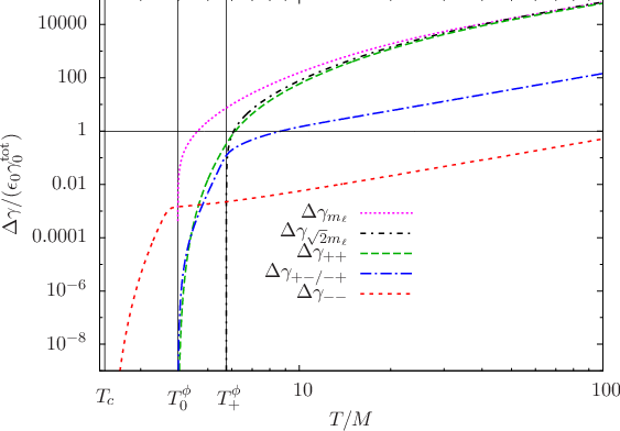
We discuss these $C\!P$ -asymmetries in detail in reference [23].

4 Boltzmann Equations

We calculate the Boltzmann equations for leptogenesis. We include decays and inverse decays involving neutrinos, leptons and Higgs bosons. We neglect all scatterings, expect the on-shell contribution of the $\Delta L=2$ scatterings, which we have to take into account for consistency reasons. We take into account thermal dispersion relations, but assume distributions close enough to equilibrium that we can use Boltzmann equations. For the distribution functions, we use the full quantum statistics, that is, Fermi-Dirac and Bose-Einstein statistics, but assume the kinetic equilibrium approximation $f_{i}=n_{i}/n_{i}^{\rm eq}f_{i}^{\rm eq}$ . It has been shown by reference [46] that this is a good approximation. The Boltzmann equations at zero temperature are derived in appendix B.

4.1 Low Temperature

Neutrino evolution

The formulation of the Boltzmann equations we need is given by equation (134) in appendix A. The equation for the evolution of the lightest right-handed neutrino reads

	$\displaystyle\frac{{\rm d}n_{N_{1}}}{{\rm d}z}=-\frac{z}{HM_{N_{1}})}$	$\displaystyle\left[\gamma(N_{1}\rightarrow\phi\ell_{+})+\gamma(N_{1}\to\bar{\phi}\bar{\ell}_{+})-\gamma(\phi\ell_{+}\to N_{1})-\gamma(\bar{\phi}\bar{\ell}_{+}\to N_{1})\right.$
	$\displaystyle+$	$\displaystyle\left.\gamma(N_{1}\rightarrow\phi\ell_{-})+\gamma(N_{1}\to\bar{\phi}\bar{\ell}_{-})-\gamma(\phi\ell_{-}\to N_{1})-\gamma(\bar{\phi}\bar{\ell}_{-}\to N_{1})\right]$		(30)

where $\ell_{\pm}$ denote the two lepton modes. We neglect scatterings since they are of higher order in the coupling constant. We will from now on omit the subscript 1 for the neutrino and write $N$ . The $CP$ -asymmetry in the matrix element is not relevant for neutrino decay, so we calculate the matrix element, which is the same for the above processes and define

\displaystyle\left|\mathcal{M}^{0}_{\pm}\right|^{2}\equiv\left|\mathcal{M}(N\to HL_{\pm})\right|^{2}=\left|\mathcal{M}(HL_{\pm}\to N)\right|^{2},

(31)

where now $HL_{\pm}$ denotes the sum of leptons and Higgs doublets, $\ell_{\pm}$ and $\phi$ , and their charge conjugated states $\bar{\ell}_{\pm}$ and $\bar{\phi}$ . The matrix elements are, however, different for the different lepton modes and also the momentum-conserving delta functions differ from each other. The subscript $\pm$ means ( $+$ ) or ( $-$ ), not the sum. When summing an expression $A_{\pm}$ that is dependent on the kind of lepton dispersion relation over the lepton modes, we write $\sum_{\pm}A_{\pm}$ . We have

\displaystyle\frac{{\rm d}n_{N}}{{\rm d}z}=-\frac{z}{H(M_{N})}\sum_{\pm}\left[\gamma(N\rightarrow HL_{\pm})-\gamma(HL_{\pm}\to N)\right]

(32)

For each of the two lepton modes, we have now

$\displaystyle\gamma(N\rightarrow HL_{\pm})-\gamma(HL_{\pm}\rightarrow N)$	$\displaystyle=\int{\rm d}\tilde{p}_{N_{1}}{\rm d}\tilde{p}_{L\pm}{\rm d}\tilde{p}_{H}(2\pi)^{4}\delta^{4}(p_{N}-p_{H}-p_{L\pm})$
	$\displaystyle\times\left[\left\|\mathcal{M}(N\rightarrow HL_{\pm})\right\|^{2}f_{N}(1+f_{H})(1-f_{L\pm})\right.$
	$\displaystyle-\left.\left\|\mathcal{M}(HL_{\pm}\rightarrow N)\right\|^{2}(1-f_{N})f_{H}f_{L\pm}\right].$	(33)

The term in square brackets in equation (33) reduces to

\left|\mathcal{M}^{0}_{\pm}\right|^{2}\left[f_{N}(1+f_{H})(1-f_{L\pm})-(1-f_{N})f_{H}f_{L\pm}\right]=\left|\mathcal{M}^{0}_{\pm}\right|^{2}\left[c_{N\rightarrow HL\pm}-c_{HL\pm\rightarrow N}\right],

(34)

where

	$\displaystyle c_{N\rightarrow HL\pm}$	$\displaystyle=f_{N}(1+f_{H})(1-f_{L\pm})\,,$
	$\displaystyle c_{HL\pm\rightarrow N}$	$\displaystyle=(1-f_{N})f_{H}f_{L\pm}\,.$		(35)

Throughout this section, we make the kinetic equilibrium assumption, that is, the phase space densities can be written as

f_{i}=\frac{n_{i}}{n_{i}^{\rm eq}}f_{i}^{\rm eq}=x_{i}f_{i}^{\rm eq},

(36)

where $x_{i}\equiv n_{i}/n_{i}^{\rm eq}$ , and $n^{\rm eq}$ and $f^{\rm eq}$ are the equilibrium number densities and distributions. For the neutrino evolution, we can assume that the Higgs bosons are in equilibrium since they couple very strongly to the thermal bath, $f_{H}=f_{H}^{\rm eq}$ . The lepton distributions of the two modes are, strictly speaking, out of equilibrium since leptons and antileptons are created asymmetrically. However, the leptons are much closer to equilibrium than the neutrinos, so the neutrino evolution is not influenced by the lepton asymmetry. Therefore we approximate the lepton densities with their equilibrium density, $f_{L\pm}=f_{L\pm}^{\rm eq}$ . We will relax this assumption in the section on the lepton asymmetry evolution.

Using the relation

f_{N}^{\rm eq}(1+f_{H}^{\rm eq})(1-f_{L\pm}^{\rm eq})=(1-f_{N}^{\rm eq})f_{L\pm}^{\rm eq}f_{H}^{\rm eq},

(37)

we can write

	$\displaystyle c_{N\rightarrow HL\pm}$	$\displaystyle=x_{N}f_{N}^{\rm eq}(1+f_{H}^{\rm eq})(1-f_{L\pm}^{\rm eq})=(x_{N}-x_{N}f_{N}^{\rm eq})f_{H}^{\rm eq}f_{L\pm}^{\rm eq}\,,$
	$\displaystyle c_{HL\pm\rightarrow N}$	$\displaystyle=(1-x_{N}f_{N}^{\rm eq})f_{H}^{\rm eq}f_{L\pm}^{\rm eq}\,,$		(38)

and

\displaystyle c_{N\rightarrow HL\pm}-c_{N\rightarrow HL\pm}

\displaystyle=(x_{N}-1)f_{H}^{\rm eq}f_{L\pm}^{\rm eq}.

(39)

The decay densities are

$\displaystyle\gamma(N\rightarrow HL_{\pm})-\gamma(HL_{\pm}\rightarrow N)$	$\displaystyle=\int{\rm d}\tilde{p}_{N}{\rm d}\tilde{p}_{L\pm}{\rm d}\tilde{p}_{H}(2\pi)^{4}\delta^{4}(p_{N}-p_{H}-p_{L\pm})$
	$\displaystyle\times\left\|\mathcal{M}_{\pm}^{0}\right\|^{2}(x_{N}-1)f_{H}^{\rm eq}f_{L\pm}^{\rm eq}$
	$\displaystyle=(x_{N}-1)\gamma_{D\pm}^{N},$	(40)

where

\displaystyle\gamma_{D\pm}^{N}=\int{\rm d}\tilde{p}_{N}{\rm d}\tilde{p}_{L\pm}{\rm d}\tilde{p}_{H}(2\pi)^{4}\delta^{4}(p_{N}-p_{H}-p_{L\pm})\left|\mathcal{M}_{\pm}^{0}\right|^{2}f_{H}^{\rm eq}f_{L\pm}^{\rm eq}.

(41)

Note that $\gamma_{D\pm}^{N}$ is not the same as the equilibrium decay density in equation (22), but differs from the latter through the thermal factor $f_{H}f_{L}$ . It is an effective decay density, which enters the Boltzmann equations. The Boltzmann equation for the neutrinos reads

\displaystyle\frac{{\rm d}n_{N}}{{\rm d}z}=-\frac{z}{H(M_{N})}(x_{N}-1)\gamma_{D}^{N},

(42)

where $\gamma_{D}^{N}\equiv\gamma_{+}+\gamma_{-}$ , or, in analogy to equation (146) in appendix B,

\displaystyle\frac{{\rm d}n_{N}}{{\rm d}z}=-D^{N}(n_{N}-n_{N}^{\rm eq}),

(43)

where

\displaystyle D^{N}=\frac{\gamma_{D}^{N}}{n_{N}^{\rm eq}}\frac{1}{Hz}

(44)

and we have used $H(M_{N})=Hz^{2}$ . Most conveniently, the number densities are normalised by the entropy density $s$ in order to factorise their dependence on the expansion of the universe. The entropy density scales as

\displaystyle s=g_{*}\frac{2\pi^{2}}{45}T^{3},

(45)

where $g_{*}$ counts the total number of effectively massless degrees of freedom and is defined as

\displaystyle g_{*}=\sum_{i={\rm bosons}}g_{i}\left(\frac{T_{i}}{T}\right)^{4}+\frac{7}{8}\sum_{i={\rm fermions}}g_{i}\left(\frac{T_{i}}{T}\right)^{4}\,,

(46)

where $i$ denotes species with mass $m_{i}\ll T$ and the factor $7/8$ arises from the difference in Fermi and Bose statistics [47]. At the temperature of leptogenesis, all SM particles have negligible masses, so $g_{*}=106.75$ . We define all number densities in terms of the entropy density as

\displaystyle Y_{i}\equiv\frac{n_{i}}{s},

(47)

then

\displaystyle x_{i}=\frac{Y_{i}}{Y_{i}^{\rm eq}}.

(48)

The Boltzmann equation reads

\displaystyle\frac{{\rm d}Y_{N}}{{\rm d}z}=-\frac{z}{sH_{1}}(x_{N}-1)\gamma_{D}^{N},

(49)

where

\displaystyle H_{1}\equiv H(T=M_{N})=\sqrt{\frac{4\pi^{3}g_{*}}{45}}\frac{M_{N}}{M_{\rm Pl}},

(50)

and the Planck mass is

\displaystyle M_{\rm Pl}=1.221\cdot 10^{19}\,{\rm GeV}.

(51)

Lepton asymmetry evolution

We set up evolution equations for the two different lepton modes separately and define the phase space density of the lepton asymmetry in the respective mode as

\displaystyle f_{\mathcal{L}h}=f_{\ell h}-f_{\bar{\ell}h}.

(52)

where $h=\pm 1$ denotes the helicity-over-chirality ratio of the leptons. The final lepton asymmetry is then $n_{\mathcal{L}}^{\rm fin}=n_{\mathcal{L}+}^{\rm fin}+n_{\mathcal{L}-}^{\rm fin}$ after evaluating the Boltzmann equations for each mode separately. The Boltzmann equations for leptons and antileptons read

$\displaystyle\frac{{\rm d}n_{\ell h_{1}}}{{\rm d}z}=-\frac{z}{H(M_{N})}\Big\{$	$\displaystyle\gamma(\ell_{h_{1}}\phi\rightarrow N)-\gamma(N\rightarrow\ell_{h_{1}}\phi)$
	$\displaystyle+\sum_{h_{2}}\left[\gamma(\ell_{h_{1}}\phi\rightarrow\bar{\ell}_{h_{2}}\bar{\phi})-\gamma(\bar{\ell}_{h_{2}}\bar{\phi}\rightarrow\ell_{h_{1}}\phi)\right]\Big\}\,,$
$\displaystyle\frac{{\rm d}n_{\bar{\ell}h_{1}}}{{\rm d}z}=-\frac{z}{H(M_{N})}\Big\{$	$\displaystyle\gamma(\bar{\ell}_{h_{1}}\bar{\phi}\rightarrow N)-\gamma(N\rightarrow\bar{\ell}_{h_{1}}\bar{\phi})$
	$\displaystyle+\sum_{h_{2}}\left[\gamma(\bar{\ell}_{h_{1}}\bar{\phi}\rightarrow\ell_{h_{2}}\phi)-\gamma(\ell_{h_{2}}\phi\rightarrow\bar{\ell}_{h_{1}}\bar{\phi})\right]\Big\},$	(53)

where we have $(h_{1},h_{2})=\pm 1$ to account for the second lepton involved in the scatterings and we have only included $\Delta L=2$ scatterings since the other two-by-two scatterings that involve only $N$ , $\ell$ and $\phi$ are negligible[15]. For the evolution of the lepton asymmetry, we have

	$\displaystyle\frac{{\rm d}n_{\mathcal{L}h_{1}}}{{\rm d}z}=$	$\displaystyle-\frac{1}{Hz}\Big\{\gamma(\ell_{h_{1}}\phi\to N)-\gamma(\bar{\ell}_{h_{1}}\bar{\phi}\to N)-\gamma(N\to\ell_{h_{1}}\phi)+\gamma(N\to\bar{\ell}_{h_{1}}\bar{\phi})$
		$\displaystyle+\sum_{h_{2}}\left[\gamma(\ell_{h_{1}}\phi\to\bar{\ell}_{h_{2}}\bar{\phi})-\gamma(\bar{\ell}_{h_{1}}\bar{\phi}\to\ell_{h_{2}}\phi)+\gamma(\ell_{h_{2}}\phi\to\bar{\ell}_{h_{1}}\bar{\phi})-\gamma(\bar{\ell}_{h_{2}}\bar{\phi}\to\ell_{h_{1}}\phi)\right]\Big\}\,.$		(54)

At leading order in the couplings, the $\Delta L=2$ scatterings are computed at tree level and are consequently $CP$ -conserving. However, from these scatterings we must subtract the $CP$ -violating contribution where an on-shell $N_{1}$ is exchanged in the $s$ channel, shown in figure 10. This is because in the Boltzmann equations the process is already taken into account by inverse decays with successive decays, $\ell\phi\to N\to\bar{\ell}\bar{\phi}$ [48, 15, 49].

We must therefore replace the scattering rate by the subtracted rate,

\gamma(\ell_{h_{1}}\phi\to\bar{\ell}_{h_{2}}\bar{\phi})\to\gamma^{\rm sub}(\ell_{h_{1}}\phi\to\bar{\ell}_{h_{2}}\bar{\phi})\equiv\gamma(\ell_{h_{1}}\phi\to\bar{\ell}_{h_{2}}\bar{\phi})-\gamma^{\rm on-shell}(\ell_{h_{1}}\phi\to\bar{\ell}_{h_{2}}\bar{\phi})

(55)

and $\gamma(\bar{\ell}_{h_{1}}\bar{\phi}\to\ell_{h_{2}}\phi)$ accordingly, where $\gamma^{\rm on-shell}$ is the on-shell contribution. The Boltzmann equations then read

$\displaystyle\frac{{\rm d}n_{\mathcal{L}h_{1}}}{{\rm d}z}=$	$\displaystyle-\frac{1}{Hz}\Big\{\gamma(\ell_{h_{1}}\phi\to N)-\gamma(\bar{\ell}_{h_{1}}\bar{\phi}\to N)-\gamma(N\to\ell\phi_{h_{1}})+\gamma(N\to\bar{\ell}_{h_{1}}\bar{\phi})$
	$\displaystyle+\sum_{h_{2}}\big[\gamma^{\rm sub}(\ell_{h_{1}}\phi\to\bar{\ell}_{h_{2}}\bar{\phi})-\gamma^{\rm sub}(\bar{\ell}_{h_{1}}\bar{\phi}\to\ell_{h_{2}}\phi)$
	$\displaystyle+\gamma^{\rm sub}(\ell_{h_{2}}\phi\to\bar{\ell}_{h_{1}}\bar{\phi})-\gamma^{\rm sub}(\bar{\ell}_{h_{2}}\bar{\phi}\to\ell_{h_{1}}\phi)\big]\Big\}\,.$	(56)

It is convenient to define a $CP$ -asymmetry in neutrino decays on amplitude level as

\epsilon^{N}_{h}=\frac{\left|\mathcal{M}(N\to\phi\ell_{h})\right|^{2}-\left|\mathcal{M}(N\to\bar{\phi}\bar{\ell}_{h})\right|^{2}}{\left|\mathcal{M}(N\to\phi\ell_{h})\right|^{2}+\left|\mathcal{M}(N\to\bar{\phi}\bar{\ell}_{h})\right|^{2}}

(57)

and $\left|\mathcal{M}(N\to\phi\ell_{h})\right|^{2}+\left|\mathcal{M}(N\to\bar{\phi}\bar{\ell}_{h})\right|^{2}=\left|\mathcal{M}_{0h}\right|^{2}$ , we write

	$\displaystyle\left\|\mathcal{M}(N\to\phi\ell_{h})\right\|^{2}=\left\|\mathcal{M}(\bar{\phi}\bar{\ell}_{h}\to N)\right\|^{2}$	$\displaystyle=\frac{1+\epsilon_{h}^{N}}{2}\left\|\mathcal{M}_{0h}\right\|^{2},$
	$\displaystyle\left\|\mathcal{M}(N\to\bar{\phi}\bar{\ell}_{h})\right\|^{2}=\left\|\mathcal{M}(\phi\ell_{h}\to N)\right\|^{2}$	$\displaystyle=\frac{1-\epsilon_{h}^{N}}{2}\left\|\mathcal{M}_{0h}\right\|^{2}.$		(58)

It is useful to write the decay rates for the above $1\leftrightarrow 2$ processes as in section 4.1,

\gamma({\rm process})=\int\prod_{j}{\rm d}\tilde{p}_{j}(2\pi)^{4}\delta^{4}\left(\sum p_{j}\right)c({\rm process}),

(59)

where $p_{j}$ denotes the relevant momenta $p_{N}$ , $p_{\ell h}=p_{\bar{\ell}h}$ and $p_{\phi}=p_{\bar{\phi}}$ and $\delta^{4}(\sum p_{j})$ the momentum conservation $\delta^{4}(p_{N}-p_{\ell h}-p_{\phi})$ . The information about the specific process is encoded in $c({\rm process})$ and we have

$\displaystyle c_{N\to\ell_{h}\phi}$	$\displaystyle=\left\|\mathcal{M}(N\to\phi\ell_{h})\right\|^{2}f_{N}(1-f_{\ell h})(1+f_{\phi})$
$\displaystyle c_{\ell_{h}\phi\to N}$	$\displaystyle=\left\|\mathcal{M}(\phi\ell_{h}\to N)\right\|^{2}(1-f_{N})f_{\ell h}f_{\phi}$
$\displaystyle c_{N\to\bar{\ell}_{h}\bar{\phi}}$	$\displaystyle=\left\|\mathcal{M}(N\to\bar{\phi}\bar{\ell}_{h})\right\|^{2}f_{N}(1-f_{\bar{\ell}h})(1+f_{\bar{\phi}})$
$\displaystyle c_{\bar{\ell}_{h}\bar{\phi}\to N}$	$\displaystyle=\left\|\mathcal{M}(\bar{\phi}\bar{\ell}_{h}\to N)\right\|^{2}(1-f_{N})f_{\bar{\ell}h}f_{\bar{\phi}}.$	(60)

Since we are looking at the lepton asymmetry, the lepton distributions have to be out of equilibrium,

$\displaystyle f_{\ell/\bar{\ell}h}$	$\displaystyle=x_{\ell/\bar{\ell}h}f_{\ell h}^{\rm eq},$
$\displaystyle f_{\mathcal{L}h}$	$\displaystyle=x_{\mathcal{L}.h}f_{\ell h}^{\rm eq},$
$\displaystyle f_{\ell h}+f_{\bar{\ell}h}$	$\displaystyle\approx 2f_{\ell h}^{\rm eq},$	(61)

while the Higgs bosons can be assumed to be in equilibrium.

As explained in appendix C, the scattering rates can be written as

$\displaystyle\sum_{h_{f}}\left[\gamma^{\rm sub}(\ell_{h_{i}}\phi\right.$	$\displaystyle\left.\to\bar{\ell}_{h_{f}}\bar{\phi})-\gamma^{\rm sub}(\bar{\ell}_{h_{i}}\bar{\phi}\to\ell_{h_{f}}\phi)\right]$
	$\displaystyle=\sum_{h_{f}}\left[\gamma^{\rm sub}(\ell_{h_{f}}\phi\to\bar{\ell}_{h_{i}}\bar{\phi})-\gamma^{\rm sub}(\bar{\ell}_{h_{f}}\bar{\phi}\to\ell_{h_{i}}\phi)\right]=$
	$\displaystyle=\int{\rm d}\tilde{p}_{N}{\rm d}\tilde{p}_{\ell h_{i}}{\rm d}\tilde{p}_{\phi}(2\pi)^{4}\delta^{4}(p_{N}-p_{\ell h_{i}}-p_{\phi})\epsilon_{h_{i}}^{N}\left\|\mathcal{M}_{h_{i}}^{0}\right\|^{2}f_{\ell h_{i}}^{\rm eq}f_{\phi}^{\rm eq}(1-f_{N}^{\rm eq}).$	(62)

so we define⁷⁷ 7 Note that our factor $c^{\rm sub}$ differs from reference [46], where they have the out-of-equilibrium distribution $(1-f_{N})$ instead of $(1-f_{N}^{\rm eq})$ . However, as derived in appendix C, we must employ $f_{N}^{\rm eq}$ , even if we had only one lepton mode, which also results in a Boltzmann equation for $(\ell-\bar{\ell})$ which is slightly different from reference [46].

\displaystyle c^{\rm sub}_{h}=2\epsilon_{h}^{N}\left|\mathcal{M}^{0}_{h}\right|^{2}f_{\ell h}^{\rm eq}f_{\phi}^{\rm eq}(1-f_{N}^{\rm eq})

(63)

and calculate the integrand for the right-hand side of the Boltzmann equation (154),

	$\displaystyle c(N\to\ell_{h}\phi)-c(\ell_{h}\phi\to N)-$	$\displaystyle c(N\to\bar{\ell}_{h}\bar{\phi})+c(\bar{\ell}_{h}\bar{\phi}\to N)+c^{\rm sub}_{h}=$
		$\displaystyle=x_{\mathcal{L}h}f_{\ell h}^{\rm eq}(f_{\phi}^{\rm eq}+x_{N}f_{N}^{\rm eq})-2\epsilon_{h}^{N}f_{\ell h}^{\rm eq}f_{\phi}^{\rm eq}\left(x_{N}-1\right)\left(1-2f_{N}^{\rm eq}\right).$		(64)

We can easily check that this term vanishes when the neutrinos are in equilibrium, $x_{N}=1$ , and there is no previous lepton asymmetry, $x_{\mathcal{L}h}=0$ .

The Boltzmann equation reads now

\displaystyle\frac{{\rm d}n_{\mathcal{L}h}}{{\rm d}z}=-\frac{1}{Hz}\left[-\epsilon^{N}_{\gamma h}\gamma_{\epsilon h}^{N}\left(x_{N}-1\right)+\frac{x_{\mathcal{L}h}}{2}\left(\gamma_{Wh}^{N}+x_{N}\gamma_{Nh}^{N}\right)\right],

(65)

where $\gamma_{Wh}^{N}=\gamma_{Dh}^{N}$ is defined in equation (41) and

$\displaystyle\gamma_{\epsilon h}^{N}$	$\displaystyle=\int{\rm d}\tilde{p}_{N}{\rm d}\tilde{p}_{\ell h}{\rm d}\tilde{p}_{\phi}(2\pi)^{4}\delta^{4}(p_{N}-p_{\phi}-p_{\ell h})\left\|\mathcal{M}_{0}\right\|^{2}f_{\phi}^{\rm eq}f_{\ell h}^{\rm eq}(1-2f_{N}^{\rm eq})$
$\displaystyle\gamma_{Nh}^{N}$	$\displaystyle=\int{\rm d}\tilde{p}_{N}{\rm d}\tilde{p}_{\ell h}{\rm d}\tilde{p}_{\phi}(2\pi)^{4}\delta^{4}(p_{N}-p_{\phi}-p_{\ell h})\left\|\mathcal{M}_{0}\right\|^{2}f_{\ell h}^{\rm eq}f_{N}^{\rm eq},$
$\displaystyle\epsilon_{\gamma h}^{N}$	$\displaystyle=\frac{1}{\gamma_{\epsilon h}}\int{\rm d}\tilde{p}_{N}{\rm d}\tilde{p}_{\ell h}{\rm d}\tilde{p}_{\phi}(2\pi)^{4}\delta^{4}(p_{N}-p_{\phi}-p_{\ell h})\epsilon_{h}^{N}\left\|\mathcal{M}_{0}\right\|^{2}f_{\phi}^{\rm eq}f_{\ell h}^{\rm eq}(1-2f_{N}^{\rm eq}).$	(66)

We see that the rates and the ${C\!P}$ -asymmetries that enter the Boltzmann equations have slightly different thermal factors than the equilibrium rate in equations (22), which employs the factor $f_{N}(1-f_{\ell})(1+f_{\phi})$ for $N$ decays.

We may also write

\displaystyle\frac{{\rm d}Y_{\mathcal{L}h}}{{\rm d}z}=-\frac{z}{sH_{1}}\left[-\epsilon^{N}_{\gamma h}\gamma_{\epsilon h}^{N}\left(x_{N}-1\right)+\frac{x_{\mathcal{L}h}}{2}\left(\gamma_{Wh}^{N}+x_{N}\gamma_{Nh}^{N}\right)\right]

(67)

or, corresponding to equation (154) in appendix B,

\displaystyle\frac{{\rm d}n_{\mathcal{L}h}}{{\rm d}z}=\epsilon_{\gamma h}^{N}D_{\epsilon h}^{N}(n_{N}-n_{N}^{\rm eq})-(W_{0h}^{N}+W_{Nh}^{N}x_{N})n_{\mathcal{L}h},

(68)

where

$\displaystyle D_{\epsilon h}^{N}$	$\displaystyle=\frac{1}{Hz}\frac{\gamma_{\epsilon h}^{N}}{n_{N}^{\rm eq}}$
$\displaystyle W_{0h}$	$\displaystyle=\frac{1}{Hz}\frac{\gamma_{Wh}^{N}}{2n_{\ell h}^{\rm eq}}$
$\displaystyle W_{Nh}$	$\displaystyle=\frac{1}{Hz}\frac{\gamma_{Nh}^{N}}{2n_{\ell h}^{\rm eq}}.$	(69)

4.2 High temperature

As discussed in section 3.1, the neutrino processes $N\leftrightarrow\ell\phi$ are forbidden when the thermal masses of the Higgs bosons and leptons become too large, that is, when $m_{\phi}>M_{N}$ . However, new processes with the Higgs as single initial or final state are then allowed, $\phi\leftrightarrow N\ell$ . These are the dominant contributions to the neutrino and lepton evolution and they can be $CP$ -violating as well, so they contribute to generating a lepton asymmetry. We derive the Boltzmann equations for this high temperature regime in the following.

Neutrino evolution

We derive the Boltzmann equation analogously to section 4.1,

\displaystyle\frac{{\rm d}n_{N}}{{\rm d}z}=-\frac{1}{Hz}\sum_{h}\left[\gamma(NL_{h}\rightarrow H)-\gamma(H\rightarrow NL_{h})\right].

(70)

We have

$\displaystyle\gamma(NL_{h}\rightarrow H)-\gamma(H\rightarrow NL_{h})$	$\displaystyle=\int{\rm d}\tilde{p}_{N}{\rm d}\tilde{p}_{Lh}{\rm d}\tilde{p}_{H}(2\pi)^{4}\delta^{4}(p_{H}-p_{N}-p_{Lh})$
	$\displaystyle\times\left[\left\|\mathcal{M}(NL_{h}\rightarrow H)\right\|^{2}f_{N}f_{Lh}(1+f_{H})\right.$
	$\displaystyle-\left.\left\|\mathcal{M}(H\rightarrow NL_{h})\right\|^{2}(1-f_{N})(1-f_{Lh})f_{H}\right].$	(71)

The tree-level matrix elements $\left|\mathcal{M}^{0}_{h}\right|^{2}$ are the same at high temperature for the Higgs-processes, just the kinematics differ. So we have

\displaystyle\left|\mathcal{M}^{0}_{h}\right|^{2}\equiv\left|\mathcal{M}(NL_{h}\rightarrow H)\right|^{2}=\left|\mathcal{M}(H\rightarrow NL_{h})\right|^{2}.

(72)

Again, we assume the Higgs bosons and leptons to be in equilibrium. We write

\displaystyle\left|\mathcal{M}_{0}\right|^{2}\left[f_{N}f_{Lh}(1+f_{H})-(1-f_{N})(1-f_{Lh})f_{H}\right]=\left|\mathcal{M}_{0}\right|^{2}\left[c(NL_{h}\rightarrow H)-c(H\rightarrow NL_{h})\right]\,.

(73)

Using the relation

\displaystyle f_{N}^{\rm eq}f_{Lh}^{\rm eq}(1+f_{H}^{\rm eq})=(1-f_{N}^{\rm eq})(1-f_{Lh}^{\rm eq})f_{H}^{\rm eq},

(74)

we get

\displaystyle c(NL_{h}\rightarrow H)-c(H\rightarrow NL_{h})=(x_{N}-1)(1-f_{Lh}^{\rm eq})f_{H}^{\rm eq}.

(75)

The Boltzmann equation then reads

\displaystyle\frac{{\rm d}n_{N}}{{\rm d}z}=-\frac{1}{Hz}(x_{N}-1)\gamma_{D}^{\phi},

(76)

\displaystyle\frac{{\rm d}Y_{N}}{{\rm d}z}=-\frac{z}{sH_{1}}(x_{N}-1)\gamma_{D}^{\phi},

(77)

\displaystyle\frac{{\rm d}n_{N}}{{\rm d}z}=-D^{\phi}(n_{N}-n_{N}^{\rm eq}),

(78)

where $\gamma_{D}^{\phi}=\gamma_{D+}^{\phi}+\gamma_{D-}^{\phi}$ ,

\displaystyle\gamma_{Dh}^{\phi}=\int{\rm d}\tilde{p}_{N}{\rm d}\tilde{p}_{Lh}{\rm d}\tilde{p}_{H}(2\pi)^{4}\delta^{4}(p_{H}-p_{N}-p_{Lh})\left|\mathcal{M}^{0}_{h}\right|^{2}f_{H}^{\rm eq}(1-f_{Lh}^{\rm eq})

(79)

and

\displaystyle D^{\phi}=\frac{\gamma_{D}^{\phi}}{n_{N}^{\rm eq}}\frac{1}{Hz}\,.

(80)

Lepton asymmetry evolution

The Boltzmann equations for leptons and antileptons read

$\displaystyle\frac{{\rm d}n_{\ell h_{1}}}{{\rm d}z}=-\frac{1}{Hz}\Big\{$	$\displaystyle\gamma(\ell_{h_{1}}N\rightarrow\bar{\phi})-\gamma(\bar{\phi}\rightarrow\ell_{h_{1}}N)$
	$\displaystyle+\sum_{h_{2}}\left[\gamma(\ell_{h_{1}}\phi\rightarrow\bar{\ell}_{h_{2}}\bar{\phi})-\gamma(\bar{\ell}_{h_{2}}\bar{\phi}\rightarrow\ell_{h_{1}}\phi)\right]\Big\},$	(81)
$\displaystyle\frac{{\rm d}n_{\bar{\ell h_{1}}}}{{\rm d}z}=-\frac{z}{H(M_{N})}\Big\{$	$\displaystyle\gamma(\bar{\ell}_{h_{1}}N\rightarrow\phi)-\gamma(\phi\rightarrow\bar{\ell}_{h_{1}}N)$
	$\displaystyle+\sum_{h_{2}}\left[\gamma(\bar{\ell}_{h_{1}}\bar{\phi}\rightarrow\ell_{h_{2}}\phi)-\gamma(\ell_{h_{2}}\phi\rightarrow\bar{\ell}_{h_{1}}\bar{\phi})\right]\Big\},$	(82)

combined we get

	$\displaystyle\frac{{\rm d}n_{\mathcal{L}h_{1}}}{{\rm d}z}=$	$\displaystyle-\frac{1}{Hz}\Big\{\gamma(\ell_{h_{1}}N\to\bar{\phi})-\gamma(\bar{\ell}_{h_{1}}N\to\phi)-\gamma(\bar{\phi}\to\ell_{h_{1}}N)+\gamma(\phi\to\bar{\ell}_{h_{1}}N)$
		$\displaystyle+\sum_{h_{2}}\left[\gamma(\ell_{h_{1}}\phi\to\bar{\ell}_{h_{2}}\bar{\phi})-\gamma(\bar{\ell}_{h_{1}}\bar{\phi}\to\ell_{h_{2}}\phi)+\gamma(\ell_{h_{2}}\phi\to\bar{\ell}_{h_{1}}\bar{\phi})-\gamma(\bar{\ell}_{h_{2}}\bar{\phi}\to\ell_{h_{1}}\phi)\right]\Big\}\,.$		(83)

At high temperature, there can be no on-shell neutrino in the $s$ -channel of the $\Delta L=2$ scatterings, but there can be an on-shell neutrino exchange in the $u$ -channel as shown in figure 11.

Again, we need to subtract the $\Delta L=2$ rates since the $u$ -channel on-shell neutrino exchange corresponds to a Higgs decay followed by an inverse decay, $\ell\phi\to\ell N\bar{\ell}\to\bar{\phi}\bar{\ell}$ . We replace

\displaystyle\gamma(\ell_{h_{1}}\phi\to\bar{\ell}_{h_{2}}\bar{\phi})\to\gamma^{\rm sub}(\ell_{h_{1}}\phi\to\bar{\ell}_{h_{2}}\bar{\phi})\equiv\gamma(\ell_{h_{1}}\phi\to\bar{\ell}_{h_{2}}\bar{\phi})-\gamma^{\rm on-shell}_{u}(\ell_{h_{1}}\phi\to\bar{\ell}_{h_{2}}\bar{\phi})

(84)

and get

	$\displaystyle\frac{{\rm d}n_{\mathcal{L}h_{1}}}{{\rm d}z}=$	$\displaystyle-\frac{1}{Hz}\Big\{\gamma(\ell_{h_{1}}N\to\bar{\phi})-\gamma(\bar{\ell}_{h_{1}}N\to\phi)-\gamma(\bar{\phi}\to\ell_{h_{1}}N)+\gamma(\phi\to\bar{\ell}_{h_{1}}N)$
		$\displaystyle+\sum_{h_{2}}\left[\gamma^{\rm sub}(\ell_{h_{1}}\phi\to\bar{\ell}_{h_{2}}\bar{\phi})-\gamma^{\rm sub}(\bar{\ell}_{h_{1}}\bar{\phi}\to\ell_{h_{2}}\phi)+\gamma^{\rm sub}(\ell_{h_{2}}\phi\to\bar{\ell}_{h_{1}}\bar{\phi})-\gamma^{\rm sub}(\bar{\ell}_{h_{2}}\bar{\phi}\to\ell_{h_{1}}\phi)\right]\Big\}\,.$		(85)

We define a $CP$ -asymmetry in Higgs decays on amplitude level as

\displaystyle\epsilon_{h}^{\phi}\equiv\frac{\left|\mathcal{M}(\bar{\phi}\to N\ell_{h})\right|^{2}-\left|\mathcal{M}(\phi\to N\bar{\ell}_{h})\right|^{2}}{\left|\mathcal{M}(\bar{\phi}\to N\ell_{h})\right|^{2}+\left|\mathcal{M}(\phi\to N\bar{\ell}_{h})\right|^{2}},

(86)

thus

	$\displaystyle\left\|\mathcal{M}(\bar{\phi}\to N\ell_{h})\right\|^{2}=\left\|\mathcal{M}(\bar{\ell}_{h}N\to\phi)\right\|^{2}=\frac{1+\epsilon_{h}^{\phi}}{2}\left\|\mathcal{M}_{h}\right\|^{2},$
	$\displaystyle\left\|\mathcal{M}(\phi\to N\bar{\ell}_{h})\right\|^{2}=\left\|\mathcal{M}(\ell_{h}N\to\bar{\phi})\right\|^{2}=\frac{1-\epsilon_{h}^{\phi}}{2}\left\|\mathcal{M}_{h}\right\|^{2}\,.$		(87)

As explained in appendix C, the scattering rates are written as

$\displaystyle\sum_{h_{f}}\left[\gamma^{\rm sub}(\ell_{h_{i}}\phi\right.$	$\displaystyle\left.\to\bar{\ell}_{h_{f}}\bar{\phi})-\gamma^{\rm sub}(\bar{\ell}_{h_{i}}\bar{\phi}\to\ell_{h_{f}}\phi)\right]$
	$\displaystyle=\sum_{h_{f}}\left[\gamma^{\rm sub}(\ell_{h_{f}}\phi\to\bar{\ell}_{h_{i}}\bar{\phi})-\gamma^{\rm sub}(\bar{\ell}_{h_{f}}\bar{\phi}\to\ell_{h_{i}}\phi)\right]$
	$\displaystyle=\int{\rm d}\tilde{p}_{N}{\rm d}\tilde{p}_{\ell h_{i}}{\rm d}\tilde{p}_{\phi}(2\pi)^{4}\delta^{4}(p_{N}-p_{\ell h_{i}}-p_{\phi})\epsilon_{h}^{\phi}\left\|\mathcal{M}_{h_{i}}^{0}\right\|^{2}f_{\ell h_{i}}^{\rm eq}(1+f_{\phi}^{\rm eq})f_{N}^{\rm eq}\,,$	(88)

\displaystyle c_{h}^{\rm sub}=2\epsilon^{\phi}_{h}\left|\mathcal{M}_{h}^{0}\right|^{2}f_{\ell h}^{\rm eq}(1+f_{\phi}^{\rm eq})f_{N}^{\rm eq}

(89)

and we get for the right-hand side of equation (85),

	$\displaystyle c(\ell_{h}N\to\bar{\phi})-$	$\displaystyle c(\bar{\ell}_{h}N\to\phi)-c(\bar{\phi}\to\ell_{h}N)+c(\phi\to\bar{\ell}_{h}N)+c_{h}^{\rm sub}$
		$\displaystyle=x_{\mathcal{L}h}f_{\ell h}^{\rm eq}(f_{\phi}^{\rm eq}+x_{N}f_{N}^{\rm eq})+2\epsilon^{\phi}_{h}(1-f_{\ell h}^{\rm eq})f_{\phi}^{\rm eq}\left(x_{N}-1\right)\left(1-2f_{N}^{\rm eq}\right).$		(90)

The Boltzmann equation reads now

\displaystyle\frac{{\rm d}n_{\mathcal{L}h}}{{\rm d}z}=-\frac{1}{Hz}\left[-\epsilon_{\gamma h}^{\phi}\gamma_{\epsilon h}^{\phi}\left(x_{N}-1\right)+\frac{x_{\mathcal{L}h}}{2}\left(\gamma_{Wh}^{\phi}+x_{N}\gamma^{\phi}_{Nh}\right)\right],

(91)

where

$\displaystyle\gamma^{\phi}_{\epsilon h}$	$\displaystyle=\int{\rm d}\tilde{p}_{N}{\rm d}\tilde{p}_{\ell h}{\rm d}\tilde{p}_{\phi}(2\pi)^{4}\delta^{4}(p_{N}-p_{\phi}+p_{\ell h})\left\|\mathcal{M}_{h}^{0}\right\|^{2}f_{\phi}^{\rm eq}(1-f_{\ell h}^{\rm eq})(1-2f_{N}^{\rm eq})$
$\displaystyle\gamma_{Wh}^{\phi}$	$\displaystyle=\int{\rm d}\tilde{p}_{N}{\rm d}\tilde{p}_{\ell h}{\rm d}\tilde{p}_{\phi}(2\pi)^{4}\delta^{4}(p_{N}-p_{\phi}+p_{\ell h})\left\|\mathcal{M}_{h}^{0}\right\|^{2}f_{\phi}^{\rm eq}f_{\ell h}^{\rm eq}$
$\displaystyle\gamma^{\phi}_{Nh}$	$\displaystyle=\int{\rm d}\tilde{p}_{N}{\rm d}\tilde{p}_{\ell h}{\rm d}\tilde{p}_{\phi}(2\pi)^{4}\delta^{4}(p_{N}-p_{\phi}+p_{\ell h})\left\|\mathcal{M}_{h}^{0}\right\|^{2}f_{\ell h}^{\rm eq}f_{N}^{\rm eq},$
$\displaystyle\epsilon^{\phi}_{\gamma h}$	$\displaystyle=\frac{1}{\gamma^{\phi}_{\epsilon h}}\int{\rm d}\tilde{p}_{N}{\rm d}\tilde{p}_{\ell h}{\rm d}\tilde{p}_{\phi}(2\pi)^{4}\delta^{4}(p_{N}-p_{\phi}+p_{\ell h})\epsilon^{\phi}_{h}\left\|\mathcal{M}_{h}^{0}\right\|^{2}f_{\phi}^{\rm eq}(1-f_{\ell h}^{\rm eq})(1-2f_{N}^{\rm eq}).$	(92)

Analogous to equation (154), we may also write

\displaystyle\frac{{\rm d}n_{\mathcal{L}h}}{{\rm d}z}=-\epsilon^{\phi}_{\gamma h}D^{\phi}_{\epsilon h}(n_{N}-n_{N}^{\rm eq})-(W^{\phi}_{0h}+W^{\phi}_{Nh}x_{N})n_{\mathcal{L}h},

(93)

where

$\displaystyle D^{\phi}_{\epsilon h}$	$\displaystyle=\frac{1}{Hz}\frac{\gamma^{\phi}_{\epsilon h}}{n_{N}^{\rm eq}}$
$\displaystyle W^{\phi}_{0h}$	$\displaystyle=\frac{1}{Hz}\frac{\gamma^{\phi}_{Dh}}{2n_{\ell h}^{\rm eq}}$
$\displaystyle W^{\phi}_{Nh}$	$\displaystyle=\frac{1}{Hz}\frac{\gamma^{\phi}_{\mathcal{L}Nh}}{2n_{\ell h}^{\rm eq}}.$	(94)

Normalised by the entropy density, the equation reads

\displaystyle\frac{{\rm d}Y_{\mathcal{L}h}}{{\rm d}z}=-\frac{z}{sH_{1}}\left[-\epsilon_{\gamma h}^{\phi}\gamma_{\epsilon h}^{\phi}\left(x_{N}-1\right)+\frac{x_{\mathcal{L}h}}{2}\left(\gamma_{Wh}^{\phi}+x_{N}\gamma^{\phi}_{Nh}\right)\right].

(95)

4.3 Interacting Modes

The Boltzmann equations in the previous sections were derived under the assumption that the only relevant interactions in which the leptons take part are the Yukawa interactions with Higgs bosons and heavy neutrinos, which have very small coupling constants $\lambda$ , while it is implicitly assumed that gauge interactions keep the leptons and the Higgs bosons in equilibrium. This scenario would imply that the two modes only interact with each other via intermediate neutrinos or Higgs bosons, where the distributions and also the asymmetries in each mode are to first approximation decoupled. In a more realistic model, the lepton modes will couple to each other via the $SU(2)$ and $U(1)$ gauge bosons $W^{a}_{\mu}$ and $B_{\mu}$ in processes like $\ell_{\pm}\to\ell_{\mp}B$ . While it is conceptually interesting to consider the case that the two modes are completely decoupled, it might be more realistic to study the scenario where the interactions between the lepton modes are fast enough to keep them in chemical equilibrium.

Chemical equilibrium implies that for species that interact via processes $a+b\to i+j$ , the corresponding chemical potentials are related as

\displaystyle\mu_{a}+\mu_{b}=\mu_{i}+\mu_{j}\,.

(96)

When the processes which create or annihilate the particles and antiparticles of some species are fast, for example via $a+\bar{a}\to i+j$ , where $i$ and $j$ are in equilibrium and their chemical potentials vanish, then the chemical potentials of $a$ and $\bar{a}$ behave as

	$\displaystyle\mu_{a}+\mu_{\bar{a}}$	$\displaystyle=\mu_{i}+\mu_{j}=0\,,$
	$\displaystyle\Rightarrow\mu_{a}$	$\displaystyle=-\mu_{\bar{a}}\,.$		(97)

In order to derive the corresponding Boltzmann equation, we introduce a chemical potential $\mu_{h}$ for the lepton mode $\ell_{h}$ . For simplicity, we approximate the distribution with Maxwell-Boltzmann statistics, an approximation which is sufficient to derive the final Boltzmann equations. The distribution functions in kinetic equilibrium are

$\displaystyle f_{\ell h}(k)$	$\displaystyle={\rm e}^{-\beta(\omega_{h}-\mu_{h})}\,,$
$\displaystyle f_{\bar{\ell}h}(k)$	$\displaystyle={\rm e}^{-\beta(\omega_{h}+\mu_{h})}\,,$
$\displaystyle f_{\ell h}(k)-f_{\bar{\ell}h}(k)$	$\displaystyle={\rm e}^{-\beta\omega_{h}}({\rm e}^{\beta\mu_{h}}-{\rm e}^{-\beta\mu_{h}})\approx 2\beta\mu_{h}f_{\ell h}^{{\rm eq}}\,,$	(98)

for $\mu_{h}\ll T$ . We assume chemical equilibrium between the plus- and the minus-mode,

\displaystyle\mu_{+}=\mu_{-}\equiv\mu_{\ell}\,.

(99)

Moreover, we can make the approximation that the equilibrium densities are about the same since the thermal mass $m_{\ell}\approx 0.2\,T$ is too small to affect the momentum integration considerably in

	$\displaystyle n_{\ell_{h}}^{\rm eq}$	$\displaystyle=\int\frac{{\rm d}^{3}k}{(2\pi)^{3}}f_{\ell_{h}}^{\rm eq}(k)\,,$
	$\displaystyle\Rightarrow n_{\ell_{+}}^{\rm eq}$	$\displaystyle\approx n_{\ell_{-}}^{\rm eq}\approx n_{\ell,0}^{\rm eq}\,,$		(100)

where $n_{\ell,0}^{\rm eq}$ is the distribution for massless leptons. With these approximations, we have

$\displaystyle n_{\mathcal{L}_{+}}$	$\displaystyle=2\beta\mu_{\ell}n_{\ell_{0}}^{\rm eq}=n_{\mathcal{L}_{-}}\,,$
$\displaystyle n_{\mathcal{L}\pm}$	$\displaystyle\equiv n_{\mathcal{L}_{+}}+n_{\mathcal{L}_{-}}\equiv 2n_{\mathcal{L}_{h}}\,,$
$\displaystyle x_{\mathcal{L}\pm}$	$\displaystyle\equiv\frac{n_{\mathcal{L}\pm}}{n_{\ell 0}^{\rm eq}}\,,$	(101)

where the subscript $\pm$ indicates that we sum over the two modes, contrary to its use in the previous sections. We can now add the Boltzmann equations for the two modes in equations (67) and (95) and arrive at

\displaystyle\frac{{\rm d}Y_{\mathcal{L}\pm}}{{\rm d}z}=-\frac{z}{sH_{1}}\left[\Delta\gamma_{\pm}\left(x_{N}-1\right)+\frac{x_{\mathcal{L}\pm}}{4}\left(\gamma_{W\pm}+x_{N}\gamma_{N\pm}\right)\right],

(102)

where

$\displaystyle Y_{\mathcal{L}\pm}$	$\displaystyle=Y_{\mathcal{L}+}+Y_{\mathcal{L}-}\,,$
$\displaystyle\Delta\gamma_{\pm}$	$\displaystyle=\epsilon_{\gamma+}\gamma_{\epsilon+}+\epsilon_{\gamma-}\gamma_{\epsilon-}\,,$
$\displaystyle\gamma_{W\pm}$	$\displaystyle=\gamma_{W+}+\gamma_{W-}\,,$
$\displaystyle\gamma_{N\pm}$	$\displaystyle=\gamma_{N+}+\gamma_{N-}\,.$	(103)

The factor $1/4$ comes from the fact that $x_{\mathcal{L}h}=x_{\mathcal{L}\pm}/2$ . Depending on the temperature regime, we either have to employ the Higgs boson or the neutrino rates in the Boltzmann equations.

4.4 One-Mode Approximation

As we did in section 3 for the decay rates and the ${C\!P}$ asymmetries, we also employ the one-mode approach for the Boltzmann equations. The equations are derived in analogy to sections 4.1 and 4.2 and read

	$\displaystyle\frac{{\rm d}Y_{N}}{{\rm d}z}$	$\displaystyle=-\frac{z}{sH_{1}}(x_{N}-1)\gamma_{Dm_{\ell}},$
	$\displaystyle\frac{{\rm d}Y_{\mathcal{L}}}{{\rm d}z}$	$\displaystyle=-\frac{z}{sH_{1}}\left[-\Delta\gamma_{m_{\ell}}\left(x_{N}-1\right)+\frac{x_{\mathcal{L}}}{2}\left(\gamma_{Wm_{\ell}}+x_{N}\gamma_{Nm_{\ell}}\right)\right],$		(104)

where $\gamma_{Dm_{\ell}}$ , $\gamma_{Wm_{\ell}}$ , $\gamma_{Nm_{\ell}}$ and $\Delta\gamma_{m_{\ell}}$ are the same as the rates defined in equations (41), (66), (79) and (92) and one has to make the appropriate replacements for the matrix elements and the lepton dispersion relations of the one-mode approach for $m_{\ell}$ and $\sqrt{2}\,m_{\ell}$ .

4.5 Evaluation of the Boltzmann Equations

We solve the Boltzmann equations for five different scenarios:

1.

the zero temperature case with Maxwell-Boltzmann statistics,
2.

the two-lepton-mode approach where the two modes do not interact with each other,
3.

the two-mode approach where the modes couple strongly to each other,
4.

the one-mode approach for a thermal mass $m_{\ell}$ ,
5.

and the one-mode approach for an asymptotic thermal mass $\sqrt{2}\,m_{\ell}$ .

In the decoupled case, the lepton asymmetries for the plus- and the minus-mode evolve separately from each other. When solving the equations, one has to specify the initial conditions for the neutrino abundance and the lepton asymmetry. We assume a vanishing initial lepton asymmetry and distinguish between three cases for the neutrino abundances:

1.

Zero initial abundance: this is the case, for example, when an inflaton field decays mostly into SM particles and not into the heavy neutrinos.
2.

Thermal initial abundance: this can be realised when some additional interactions keep the neutrinos in equilibrium at $T\gg M_{1}$ , for example via a heavy $Z^{\prime}$ boson related to $SO(10)$ unification [50].
3.

Dominant initial abundance: this is the case, for example, when an inflaton decays predominantly into $N_{1}$ .

The coupling $(\lambda^{\dagger}\lambda)_{11}$ , which enters the neutrino decay rate, is parameterised by the so-called decay parameter $K$ , defined as

\displaystyle K\equiv\frac{\widetilde{m}_{1}}{m^{*}}\,,

(105)

where

\displaystyle\widetilde{m}_{1}=\frac{(\lambda^{\dagger}\lambda)_{11}v^{2}}{M_{1}}

(106)

is the conveniently defined effective neutrino mass, which is of the order of the light neutrino mass scale, and

\displaystyle m^{*}=\left.8\pi\frac{v^{2}}{M_{1}^{2}}H\right|_{T=M_{1}}\simeq 1.1\times 10^{-3}\,{\rm eV}\,

(107)

is called equilibrium neutrino mass. In the language of these masses, the out-of-equilibrium condition, $\Gamma<H$ , corresponds to $K>1$ and is called strong washout regime. The case $K<1$ is called weak washout regime.

We want to analyse the evolution of the neutrino abundance and lepton asymmetries for the weak and strong washout regimes and different initial abundances. To this end, we write the Boltzmann equations for the different scenarios in the form of equations (43), (68), (78) and (93),

	$\displaystyle\frac{{\rm d}Y_{N}}{{\rm d}z}$	$\displaystyle=-D(Y_{N}-Y_{N}^{\rm eq})\,.$
	$\displaystyle\frac{{\rm d}Y_{\mathcal{L}}}{{\rm d}z}$	$\displaystyle=\epsilon_{0}D_{\epsilon}(Y_{N}-Y_{N}^{\rm eq})-(W+W_{N}x_{N})Y_{\mathcal{L}}\,,$		(108)

where

	$\displaystyle D$	$\displaystyle=\frac{z}{H_{1}}\frac{\gamma_{D}}{sY_{N}^{\rm eq}}\,,$	$\displaystyle D_{\epsilon}$	$\displaystyle=\frac{z}{H_{1}}\frac{\Delta\gamma}{\epsilon_{0}sY_{N}^{\rm eq}}\,,$
	$\displaystyle W$	$\displaystyle=\frac{z}{H_{1}}\frac{\gamma_{W}}{2sY_{\mathcal{L}}^{\rm eq}}\,,\quad$	$\displaystyle W_{N}$	$\displaystyle=\frac{z}{H_{1}}\frac{\gamma_{N}}{2sY_{\mathcal{L}}^{\rm eq}}\,.$		(109)

One usually refers to $D_{\epsilon}(Y_{N}-Y_{N}^{\rm eq})$ as source term since this term is responsible for the production of a lepton asymmetry. The term $(W+W_{N}x_{N})Y_{\mathcal{L}}^{\rm eq}$ is called washout term since it usually has the opposite sign as the source term and reduces the production of the lepton asymmetry. The terms $D$ , $D_{\epsilon}$ , $W$ and $W_{N}$ are different for the different scenarios. Note that for the finite temperature cases, $D_{\epsilon}$ is not the same as $D$ and there is an additional washout term $W_{N}$ due to the quantum statistics. Our analysis closely follows the arguments and explanations in reference [49] and the interested reader will find a comprehensive explanation of leptogenesis dynamics in the vacuum case therein.

Weak washout for zero initial abundance

Let us start with the weak washout regime and zero initial abundance. We define a value $z_{\rm eq}$ by the condition

\displaystyle Y_{N}(z_{\rm eq})=Y_{N}^{\rm eq}(z_{\rm eq})\,.

(110)

For $z\ll 1$ , the neutrino abundance is negligible compared to $Y_{N}^{\rm eq}$ ,

\displaystyle\frac{{\rm d}Y_{N}}{{\rm d}z}\simeq DY_{N}^{\rm eq}\,,

(111)

where $Y_{N}^{\rm eq}$ is approximately constant for $z\ll 1$ . The entropy density $s$ is proportional to $z^{-3}$ and $\gamma_{D}$ is proportional to $z^{-2}$ in vacuum and $z^{-4}$ for the Higgs boson decays at high temperature in the finite temperature cases. Thus $D\sim z^{2}$ in the vacuum case and $D\sim{\rm const.}$ at finite temperature. Neglecting $Y_{N}^{\rm initial}$ and $z^{\rm initial}$ , the integration yields $Y_{N}\simeq zD(z)/3\sim z^{3}$ for the vacuum case and $Y_{N}\simeq zD\sim z$ for the finite temperature cases. We show the numerical results for $K=0.005$ and zero initial abundance in figures 12 and 13, where these power laws for $Y_{N}(z)$ can be observed for $z\lesssim 0.1$ . We also see that $Y_{N}^{m_{\ell}}>Y_{N}^{\sqrt{2}\,m_{\ell}}>Y_{N}^{\pm}\gg Y_{N}^{0}$ , which reflects $\gamma_{D}^{m_{\ell}}>\gamma_{D}^{\sqrt{2}\,m_{\ell}}>\gamma_{D}^{\pm}\gg\gamma_{0}$ . Between the thresholds $z_{+}^{\phi}$ and $z_{+}^{N}$ , the finite-temperature abundances do not evolve much, which reflects that the decay rates are very low or vanishing in this regime. The neutrino abundance for the asymptotic mass $\sqrt{2}\,m_{\ell}$ does not rise at all at high temperature, while $Y_{N}^{m_{\ell}}$ rises slightly between $z_{0}^{\phi/N}$ and $z_{+}^{\phi/N}$ , where the rate is non-zero. The two-mode rate $\gamma_{\pm}$ is, though very suppressed, present over the whole threshold range between $z_{+}^{\phi}$ and $z_{+}^{N}$ due to the minus-modes, so $Y_{N}^{\pm}$ rises slightly. At low temperature, $z>z_{\rm eq}$ , the neutrino abundances of the different scenarios are very close to each other, since for $z\gtrsim 2$ , the rates are very close to the vacuum rate, $\gamma_{D,W,N}^{T>0}\simeq\Delta\gamma^{T>0}/\epsilon_{0}\simeq\gamma_{0}$ . In this regime, $Y_{N}$ is much larger than $Y_{N}^{\rm eq}$ since the coupling is too small to keep the abundance close to equilibrium.

Having outlined the evolution of the neutrino abundance at high temperature, we can understand the evolution of the lepton asymmetry at high temperature. The washout term in the Boltzmann equations proportional to $Y_{\mathcal{L}}$ is much smaller than the source term $D_{\epsilon}(Y_{N}-Y_{N}^{\rm eq})$ , since $Y_{\mathcal{L}}/\epsilon_{0}\ll Y_{N}^{\rm eq}$ , and we have for $z\ll z_{\rm eq}$ ,

	$\displaystyle Y_{\mathcal{L}}^{T>0}$	$\displaystyle\simeq-z\epsilon_{0}D_{\epsilon}\,$
	$\displaystyle Y_{\mathcal{L}}^{T=0}$	$\displaystyle\simeq-z\epsilon_{0}\frac{D_{\epsilon}(z)}{3}\,.$		(112)

In the high temperature regime, the lepton asymmetry is negative and follows the neutrino abundance in its absolute value,

\displaystyle Y_{\mathcal{L}}(z)\simeq-\epsilon_{0}\frac{D_{\epsilon}}{D}Y_{N}(z)=-\frac{\Delta\gamma}{\gamma_{D}}Y_{N}(z)\,.

(113)

For the vacuum case, $D_{\epsilon}\equiv D$ and $Y_{\mathcal{L}}/\epsilon_{0}\simeq-Y_{N}$ , while for the finite temperature cases, $D_{\epsilon}/D=\Delta\gamma/(\epsilon_{0}\gamma_{D})\sim\mathcal{O}(10^{1})$ .⁸⁸ 8 We saw in section 3.2 that $\Delta\gamma/(\epsilon_{0}\gamma_{D})\sim\mathcal{O}(10^{2})$ at high temperature instead of $\mathcal{O}(10^{1})$ . The discrepancy is due to rates and asymmetries that occur in the Boltzmann equations and that are slightly different from the usual rates and ${C\!P}$ -asymmetries in section 3 due to the different statistical factors they employ, for example $1$ in equation (79) or $(1-2f_{N}^{\rm eq})$ in equation (92) instead of the usual factor $(1-f_{N}^{\rm eq})$ in equation (23). Both behaviours can be observed in figures 12 and 13. The lepton asymmetry in the minus-mode obeys the same power law as the other finite-temperature modes, but is about a factor $100$ lower due to the lower rates. The combined ( $\pm$ )-abundance closely follows the plus-abundance since the influence of the minus-mode rates is very suppressed and also the different washout term with factor $1/4$ instead of $1/2$ can be neglected.

Before turning to the intermediate temperatures $z\sim z_{\rm eq}$ , let us discuss the low temperature regime. For $z>z_{\rm eq}$ , $Y_{N}\gg Y_{N}^{\rm eq}$ , so the source term dominates and washout can be neglected. Since in this regime, $D_{\epsilon}^{T>0}\simeq D^{T>0}\simeq D^{T=0}$ , we can write

\displaystyle\frac{{\rm d}Y_{\mathcal{L}}}{{\rm d}z}\simeq\epsilon_{0}D(Y_{N}-Y_{N}^{\rm eq})=-\epsilon\frac{{\rm d}Y_{N}}{{\rm d}z}\,.

(114)

To first order, the negative lepton asymmetry created below $z_{\rm eq}$ and the positive contribution from above $z_{\rm eq}$ have the same magnitude and cancel each other. For the remaining asymmetry that did not cancel, the washout contribution up to $z_{\rm eq}$ and the exact behaviour of the abundances around $z_{\rm eq}$ are crucial.

Assuming that $Y_{N}(z=\infty)=0$ , we get

\displaystyle Y_{\mathcal{L}}^{\rm fin}\simeq\epsilon_{0}Y_{N}(z_{\rm eq})-|Y_{\mathcal{L}}(z_{\rm eq})|\,,

(115)

so we see that the evolution of the difference $\Delta Y(z)\equiv Y_{N}(z)-|Y_{\mathcal{L}}(z)|/\epsilon_{0}$ below $z_{\rm eq}$ is crucial for the final lepton asymmetry. For the regime $1\lesssim z\lesssim z_{\rm eq}$ , we can write

	$\displaystyle\frac{{\rm d}\Delta Y}{{\rm d}z}$	$\displaystyle\simeq Y_{N}^{\rm eq}(D-D_{\epsilon})\,,$
	$\displaystyle D-D_{\epsilon}$	$\displaystyle=\frac{z}{H_{1}}\frac{1}{sY_{N}^{\rm eq}}\left(\gamma_{D}-\frac{\Delta\gamma}{\epsilon}\right)\,.$		(116)

For the finite-temperature cases, the ${C\!P}$ -asymmetry in the decay rates, $\Delta\gamma/\epsilon_{0}$ , is considerably smaller than the decay rate $\gamma_{D}$ in the range $z_{0}^{N}\lesssim z\lesssim 2$ , which can be seen in figure 8. Moreover, for the one-mode cases, $\Delta\gamma_{m}/\epsilon_{0}$ approaches $\gamma_{m}$ faster than $\Delta\gamma_{++}$ approaches $\gamma_{+}$ for the plus-mode. Above $z_{+}^{N}$ , the ratio $\Delta\gamma/(\epsilon_{0}\gamma_{D})$ for the two one-mode cases is about the same. Thus, the difference $\Delta D\equiv D-D_{\epsilon}$ is largest for the two-mode approach, smaller and about the same for the two one-mode approaches and vanishing for the vacuum approach, $\Delta D^{+}>\Delta D^{m_{\ell}}\simeq\Delta D^{\sqrt{2}\,m_{\ell}}$ and $\Delta D^{0}=0$ . As a result, $\Delta Y^{+}\gtrsim\Delta Y^{m_{\ell}}\simeq\Delta Y^{\sqrt{2}\,m_{\ell}}$ at $z_{\rm eq}$ and therefore the final asymmetries are related as $Y_{\mathcal{L}}^{+}>Y_{\mathcal{L}}^{m_{\ell}}\simeq Y_{\mathcal{L}}^{\sqrt{2}\,m_{\ell}}\gg Y_{\mathcal{L}}^{0}$ . Note that the final asymmetry is non-vanishing for the vacuum case, since the washout at higher temperature is larger than at lower temperature due to the larger decay rate. For the finite temperature cases, the difference $D-D_{\epsilon}$ in the crucial regime $z\simeq z_{\rm eq}$ governs the final asymmetry.

The evolution of the decoupled minus-mode at low temperature is very different but not hard to understand. The asymmetry rises at $z\gtrsim z_{+}^{N}$ , because this is the regime above $z_{c}$ where $\Delta\gamma_{-+}$ is maximal and therefore $D_{\epsilon}^{-}$ is maximal as well. Between the thresholds $z_{+}^{\phi}$ and $z_{+}^{N}$ , $\Delta\gamma_{-+}$ is suppressed by the internal plus-lepton and $\Delta\gamma_{--}$ is suppressed by the residue of the internal minus-lepton, so $D_{\epsilon}$ is negligible and $Y_{\mathcal{L}}^{-}$ does not rise. Above $z\sim 1$ , $\Delta\gamma_{-+}$ falls due to the residue of the external minus-mode and $Y_{\mathcal{L}}^{-}$ does not change. The final lepton asymmetry therefore does not change its sign above $z\gtrsim z_{\rm eq}$ and keeps the value it achieves at around $1\lesssim z\lesssim 2$ where the ${C\!P}$ -asymmetry $\Delta\gamma_{-+}$ becomes small.

The combined ( $\pm$ )-mode does not evolve differently from the plus-mode since the influence from the $\gamma_{-}$ rates can be neglected and also the washout term with the additional factor $1/2$ is not noticeable since washout is very small in all temperature regimes. Summarising, there are four differing lepton asymmetries in this regime: the vacuum case, the $m_{\ell}$ -case, the ( $+$ )-case and the ( $-$ )-case. The $\sqrt{2}\,m_{\ell}$ -case yields the same asymmetry as the $m_{\ell}$ -case and the ( $\pm$ )-case yields the same asymmetry as the ( $+$ )-case. We show the four differing lepton asymmetries together in figure 14.

Strong and intermediate washout for zero initial abundance

For strong washout, the evolution of the neutrino abundance is analogous to the weak washout regime, with $Y_{N}^{T}\sim z$ and $Y_{N}^{0}\sim z^{3}$ , as shown in figures 15 and 16. The couplings are stronger, therefore the abundances rise faster and meet $Y_{N}^{\rm eq}$ earlier at $z_{\rm eq}\sim 1$ . For larger $z$ , the couplings are strong enough to keep $Y_{N}$ close to equilibrium. The evolution of the lepton asymmetry is nicely explained in reference [49] for the vacuum case with some rather accurate analytical approximations. In this work, we are only interested in the difference of the vacuum case to the finite temperature case. In the strong washout regime, the lepton asymmetries rise rather fast and the washout term, which competes with the source term, becomes larger than the latter at some temperature $z_{\rm min}$ , where the lepton asymmetry reaches its most negative value. The source term becomes small when $Y_{N}$ approaches its equilibrium value, so the washout term drives the asymmetry evolution back to zero. At $z\gtrsim z_{\rm eq}$ , the neutrino abundance slightly overshoots $Y_{N}^{\rm eq}$ , so the source term changes sign and adds to the washout term until the lepton asymmetry becomes positive, where the washout term changes its sign as well and is competing again. At low temperature, source term and washout term have the same magnitude when the lepton asymmetry reaches a maximum at $z_{\rm max}$ . Above $z_{\rm max}$ , the lepton asymmetry is again driven to zero by the larger washout. At very low temperature, washout and source term become very small and do not influence the asymmetry further, which settles at a final value $Y_{\mathcal{L}}^{\rm fin}$ . We see that in the strong washout regime, the dynamics are governed by the washout term. The evolution of the finite temperature lepton asymmetries is analogous to the vacuum case, but they settle to a different final value. For the finite temperature cases, the equilibrium density of leptons is smaller than in the vacuum case due to the thermal mass $m_{\ell}\sim 0.2\,T$ . The washout term is effectively larger than for the vacuum case and competes with the source term in a stronger way. Therefore, the asymmetry evolution appears slightly damped compared to the vacuum case and the final asymmetry is marginally lower. The evolution of the minus-mode is analogous to the evolution at weak washout, rises fast below $z_{+}^{\phi}$ and does not change above the thresholds since $Y_{N}\sim Y_{N}^{\rm eq}$ in this regime. The combined ( $\pm$ )-mode tracks the plus-mode until washout becomes relevant at $z\gtrsim z_{\rm eq}$ . The washout term for the ( $\pm$ )-mode is always about a factor two smaller than for the plus-mode, since we add the minus- and plus-washout rates, where the minus-rate is always negligible compared to the plus-rate. Thus, the ( $\pm$ )-abundance is less affected by washout, so the dynamics are affected by the source term in a stronger way and the final asymmetry is larger. We can view this behaviour as always distributing half the asymmetry in a mode $\ell_{-}$ which couples strongly to $\ell_{+}$ and is not affected by washout. The final asymmetry is about a factor two larger than for the other scenarios in the strong washout regime.

The case of intermediate washout is shown in figure 17, where we only show the two-mode cases since in this regime, the final lepton asymmetries of the one-mode cases are the same as for the plus-mode. The dynamics can be viewed as an interpolation between the strong and weak washout regimes and the final asymmetries are very similar to each other.

Non-zero initial abundance

We also present the dynamics for thermal and dominant initial abundance in figures 18–23.

For weak washout and thermal initial abundance, $Y_{N}\gg|Y_{\mathcal{L}}|$ for low temperatures, and according to equation (115), $Y_{\mathcal{L}}^{\rm final}/\epsilon_{0}\sim Y_{N}^{\rm initial}$ . For weak washout and dominant initial abundance, this equation holds as well, as can be seen in figures 18 and 19. For intermediate washout $K\sim 1$ and dominant abundance, shown in figures 20 and 21, the lepton asymmetry production is stopped between the thresholds for the thermal cases and the production above $z\sim 1$ does not succed in producing an asymmetry as high as in the vacuum case. For the ( $\pm$ )-case, the asymmetry production is larger since it is not as much affected by washout.

For the strong washout regime and large initial neutrino abundances, the dynamics at high temperature are interesting, as shown in figures 22 and 23, but the interplay between source term and washout term at low temperature governs the final asymmetry as in the zero-abundance case. We reproduce the well-known fact that the initial conditions do not influence the final asymmetry in the strong washout regime, while the arguments concerning the equilibrium distribution of leptons with thermal mass and the reduced washout of the ( $\pm$ )-mode still hold and lead to the same lepton asymmetry as for zero initial abundance. The decoupled minus-mode is very much affected by the coupling, that is the decay parameter $K$ , and the initial conditions, since the final lepton asymmetry is produced at high temperatures. The stronger the coupling, the larger the asymmetry production of the minus-mode at high temperatures and the larger the final value. Moreover, the larger the initial deviation of the neutrino abundance from equilibrium, the larger the asymmetry production and the final asymmetry. The final lepton asymmetry in this mode is thus lowest for neutrinos with thermal initial abundance.

Final lepton asymmetries

The values of the final asymmetries are shown in figures 24–26 for different initial abundances.

For zero initial abundance and weak washout, shown in figure 24, the asymmetries for the finite-temperature cases are larger than for the vacuum case by about one order of magnitude due to the difference of the thermal rates $\gamma_{D}$ and the ${C\!P}$ -asymmetries $\Delta\gamma$ at $z\gtrsim z_{+}^{N}$ . The lepton asymmetry for the plus-mode is also slightly larger than for the one-mode cases due to a suppression of the ${C\!P}$ asymmetry compared to the one-mode approaches. For strong washout, the asymmetry production in the vacuum case is marginally more efficient than in the thermal cases due to a smaller lepton equilibrium distribution, while the lepton asymmetry in the ( $\pm$ )-approach is by a factor two larger than in the other cases since half of the asymmetry is stored in the $\ell_{-}$ -modes and not affected by washout. The minus-mode case is completely decoupled, the lepton asymmetry bears the opposite sign as the other lepton asymmetries and rises with stronger couplings, that is with larger decay parameter $K$ . As discussed in section 4.3, this scenario might not be realistic since the modes will couple to each other via gauge bosons, so an evolution similar to the ( $\pm$ )-case seems more likely.

For thermal initial abundance and weak washout, shown in figure 25, the final asymmetry equals the equilibrium abundance $Y_{\mathcal{L}}/\epsilon_{0}$ , while in the strong washout regime, it shows the same behaviour as in the case of zero initial neutrino abundance. The minus-mode asymmetry is very low for thermal initial neutrino abundance since the neutrinos are close to equilibrium at high temperatures. Contrary to the zero initial abundance case, it bears the same sign as the lepton asymmetries of the other scenarios.

For dominant initial abundance, shown in figure 26, the final lepton asymmetries assume their maximal value in the weak washout regime, when the coupling is weak enough not to wash them out at low temperature. For larger couplings $K\sim 1$ , the thresholds lead to a halted asymmetry production for the finite temperature cases and not as much asymmetry can be produced as for the vacuum case. The ( $\pm$ )-case shows a larger asymmetry compared to the other thermal cases due to the weaker washout. At strong coupling $K\gg 1$ , the asymmetries are the same as for thermal and zero initial neutrino abundance. The minus-mode asymmetry is large in all washout regimes, since the neutrinos are far from equilibrium at high temperatures when the $\ell_{-}$ -asymmetry is produced.

A summary of the several initial conditions can be seen in figure 27, where we have omitted the $\sqrt{2}\,m_{\ell}$ case since it is very close to the $m_{\ell}$ case in all scenarios. In the weak washout regime, the case with zero initial abundance is most strongly affected by thermal corrections which amount to one order of magnitude, and the plus-mode asymmetry is additionally enhanced by a factor of about two. In the intermediate regime, the dominant-initial-abundance case is influenced very much by thermal corrections. Therefore, a production mechanism for dominant neutrino abundance has to take into account such thermal effects. In the strong washout regime, one would naturally expect that thermal corrections can be neglected. We see that this is not the case since for strongly interacting leptonic quasiparticles, a part of the lepton asymmetry can be hidden in the $\ell_{-}$ -mode which is unaffected by washout, thus producing an asymmetry by up to a factor of two larger than at zero temperature. The effect of the thermal lepton mass on the equilibrium distribution of the leptons is an interesting feature, but very small and can be neglected for all practical purposes.

5 Conclusions

For a minimal and self-consistent toy model of leptogenesis, which consists only of neutrinos, leptons and Higgs bosons, we have performed an extensive analysis of the effects of HTL corrections. This implies capturing the effects of thermal masses, modified dispersion relations and modified helicity structures. We put special emphasis on the influence of the two fermionic quasiparticles, which show a different behaviour than particles in vacuum, notably through their dispersion relations, but also the helicity structure of their interactions. Our work is thus similar to the work done in reference [15], where the authors of the latter work did not include the effects of fermionic quasiparticles and get a different result for the ${C\!P}$ -asymmetries, which are crucial for the evolution of the lepton asymmetry. Our toy model produces two lepton asymmetries stored in the two different lepton modes without the possibility of an equilibration of these asymmetries by SM processes. Since we expect the lepton modes to interact via gauge bosons in the bath, we examine a second case where the modes are strongly coupled to each other. As a third and fourth case, we approximate the lepton propagators by zero temperature propagators with the zero temperature mass replaced by the thermal lepton mass in one case and the asymptotic mass in the other case. We refer to these cases as one-mode approach. All four thermal cases are compared to the zero-temperature case.

We have calculated interaction rates and $C\!P$ -asymmetries in references [24], [25] and [23], where a detailed analysis can be found. We present the rates and $C\!P$ -asymmetries shortly in section 3. Neglecting the zero-temperature fermion mass, the resummation of HTL fermion self-energies results in an effective fermion propagator that does not break chiral invariance and is split up into two helicity modes. The external fermion states therefore behave conceptually different from the ones with chirality-breaking thermal masses that have been inserted in the kinematics by hand. Moreover, one has to take care of one additional mode, which has implications for the Boltzmann equations.

We derive and evaluate the Boltzmann equations in section 4, performing the crucial subtraction of on-shell intermediate states in appendix C⁹⁹ 9 Reference [46] uses a thermal factor $(1-f_{N})$ without explicitly deriving this factor. We show in this appendix that we have to use the equilibrium distribution for the neutrinos in $(1-f_{N}^{\rm eq})$ instead.. We compare the results of the Boltzmann equations for our five cases, that is, decoupled lepton modes, strongly coupled lepton modes, the one-mode approach with $m_{\ell}$ , the one-mode approach with $\sqrt{2}\,m_{\ell}$ , and the vacuum case. We assume three different initial values for the abundance of neutrinos: zero, thermal and dominant abundance, motivated by different scenarios for the production of heavy neutrinos after inflation [15]. In the weak washout regime, we find that using thermal masses enhances the final lepton asymmetry by about one order of magnitude for zero initial neutrino abundance. This is due to the fact that the ${C\!P}$ -asymmetry and the decay rate evolve differently at $z\gtrsim 1$ when using thermal masses, since the ${C\!P}$ -asymmetry suffers from an additional suppression by thermal masses through the leptons and Higgs bosons in the loop. Due to the helicity structure of the modes, the ${C\!P}$ -asymmetry of the plus-mode is additionally suppressed, which results in an additional enhancement of the plus-mode lepton asymmetry compared to the final asymmetries of the one-mode approaches. The enhancement we find is similar to the one found in reference [15] in this regime, but hard to compare quantitatively due to their different approach, which includes scatterings, and the discrepancy in the ${C\!P}$ -asymmetry.

In the strong washout regime, thermal masses do not show an influence, as expected¹⁰¹⁰ 10 There is a slight suppression of the lepton asymmetry for thermal masses, since the thermal mass suppresses the equilibrium distribution of the leptons somewhat and thereby enhances the washout term.. However, when we couple the plus- and minus-mode strongly, we observe an enhancement of the lepton asymmetry by a factor of about two, since we stored half of the asymmetry in a mode that essentially does not interact with the neutrinos and is therefore not affected by washout. For intermediate washout, that is $K\sim 1$ , we find that the lepton asymmetries with thermal masses are about one magnitude lower than in the vacuum case when we assume dominant initial neutrino abundance. This is due to the fact that the lower ${C\!P}$ -asymmetry does not succeed in producing as much lepton asymmetry at $z\gtrsim 1$ when using thermal masses.

A decoupled minus-mode would show a behaviour completely different from the other thermal cases and the vacuum case for all initial values of the neutrino abundance. The lepton asymmetry in such a decoupled mode is produced mainly at high temperature and only slightly affected by the development at $z\gtrsim 1$ , where it decouples from the evolution of the other abundances. Therefore, the washout parameter $K$ , which determines the coupling strength and thereby the asymmetry production at high temperatures, is crucial for the final value of the lepton asymmetry in this mode, as is the initial neutrino abundance.

Summarising, we argue that for an accurate description of medium effects on leptogenesis, the influence of thermal quasiparticles, notably the effects of the two fermionic modes, cannot be neglected. Similar to reference [15], our study shows that thermal masses have a strong effect in the weak washout regime, while the effect of fermionic modes has an additional influence on the final lepton asymmetry in this regime. We also showed that notably in the strong washout regime, the presence of a quasi-sterile lepton mode that is not affected by washout can have a non-negligible effect on the final lepton asymmetry. Future studies should clarify the dynamics of the interaction between the two fermionic modes and determine whether the evolution of the asymmetries in the two modes is closer to the decoupled or the strongly coupled case.

Another important aspect that might be studied in future works is the influence of the finite width of the fermionic modes [51], notably the minus-mode. Such effects could be studied using formalism that takes into account non-equilibrium quantum effects, such as Kadanoff-Baym equations [52, 53, 54, 55, 22, 20, 18, 16, 19, 56, 57]. In the quest for a unified description of finite-temperature effects on leptogenesis, it is important to include SM interactions in the Kadanoff-Baym studies that are under way. To this end, quasiparticle excitations of fermions and gauge-bosons should be taken into account. Last but not least, the fermionic modes might have an influence on other related dynamics in the early universe that involve fermions, such as thermal production of axions, axinos or gravitinos, which could be studied in future works.

Acknowledgements

We would like to thank Mathias Garny, Georg Raffelt, Michael A. Schmidt and Markus Thoma for their support and comments in this project. Thanks also to Denis Besak, Dietrich Bödeker, Wilfried Buchmüller, Valerie Domcke, Marco Drewes, Andreas Hohenegger, Alexander Kartavtsev and Christoph Weniger for fruitful and inspiring discussions.

Appendix A Particle Kinematics

The Boltzmann equations describe the time evolution of the distribution function of a particle species $\psi$ . We assume an isotropic and spatially homogeneous universe described by the Friedmann-Lemaitre-Robertson-Walker (FLRW) metric [47],

{\rm d}s^{2}={\rm d}t^{2}-a(t)^{2}\left\{\frac{{\rm d}r^{2}}{1-kr^{2}}+r^{2}{\rm d}\theta^{2}+r^{2}\sin^{2}\theta{\rm d}\phi^{2}\right\},

(117)

where $a(t)$ is the cosmic scale factor, which describes the expansion of the universe, $k=\pm 1,0$ specifies the curvature, and $(t,r,\theta,\phi)$ are the comoving coordinates.

The trajectory of a particle $\psi$ with mass $m_{\psi}\geq 0$ moving in a gravitational field is given by the geodesic equations of motion [58]:

	$\displaystyle\frac{{\rm d}p_{\psi}^{\mu}}{{\rm d}\tau}+\Gamma^{\mu}_{\nu\alpha}\,p_{\psi}^{\nu}\,p_{\psi}^{\alpha}$	$\displaystyle=0,$		(118)
	$\displaystyle\frac{{\rm d}x_{\psi}^{\mu}}{{\rm d}\tau}$	$\displaystyle=p_{\psi}^{\mu}.$		(119)

Since $s=m_{\psi}\tau$ is the eigen-time of the particle, $\tau$ is fixed and $p^{\mu}$ is the momentum of a particle $\psi$ .

In the FLRW metric the $\mu=0$ component of Eq (118) is given as

\displaystyle\frac{{\rm d}p_{\psi}^{0}}{{\rm d}\tau}+\frac{\dot{a}}{a}\mathbf{p}_{\psi}^{2}=0,\ \qquad\textrm{with}\quad\dot{a}=\frac{\partial a}{\partial t}.

(120)

Writing $p_{\psi}^{0}\,{\rm d}p_{\psi}^{0}=|\mathbf{p}_{\psi}|\,{\rm d}|\mathbf{p}_{\psi}|$ , this leads to:

⇔	$\displaystyle\|\dot{\mathbf{p}}_{\psi}\|a+\dot{a}\|\mathbf{p}_{\psi}\|=0$
$\displaystyle\Leftrightarrow$	$\displaystyle\frac{{\rm d}}{{\rm d}t}(\|\mathbf{p}_{\psi}\|a)=0$
$\displaystyle\Leftrightarrow$	$\displaystyle\|\mathbf{p}_{\psi}\|={\rm const.}\times\frac{1}{a}.$	(121)

Therefore the 3-momentum scales as $1/a$ .

In general, the Liouville operator describing the evolution of a point particle’s phase space in a gravitational field is given by

\displaystyle L=p^{\alpha}\frac{\partial}{\partial x^{\alpha}}-\Gamma{{}^{\alpha}_{\beta\gamma}}p^{\beta}p^{\gamma}\frac{\partial}{\partial p^{\alpha}}.

(122)

With this operator the equations of motion (118) and (119) can be written for the momentum as

\displaystyle\frac{{\rm d}p^{\mu}}{{\rm d}\tau}=L\left[p^{\mu}\right],

(123)

and for the space-time as

\displaystyle\frac{{\rm d}x^{\mu}}{{\rm d}\tau}=L\left[x^{\mu}\right].

(124)

Furthermore, the time derivative of the phase space distribution of a non-interacting gas vanishes,

\displaystyle\frac{{\rm d}f(x,p)}{{\rm d}\tau}=0.

(125)

Using the equations of motion for the particle we obtain the Boltzmann equations for the non-interacting particle species $\psi$ ,

\displaystyle L\left[f_{\psi}(x,p)\right]=0.

(126)

Since we assume a Robertson–Walker universe which is isotropic and homogeneous, the distribution function $f_{\psi}$ depends only on $t$ and $|\mathbf{p}_{\psi}|$ . Therefore, the Boltzmann equation can be written as [47]

\displaystyle L\left[f_{\psi}\right]=E_{\psi}\frac{\partial f_{\psi}}{\partial t}-H|\mathbf{p}_{\psi}|^{2}\frac{\partial f_{\psi}}{\partial E_{\psi}}=0,

(127)

where we have omitted arguments for the sake of notational clarity.

Since $p_{\psi}^{2}=m_{\psi}^{2}$ and because of the spatial isotropy of the Robertson–Walker–Metric, we have

\displaystyle|\mathbf{p}_{\psi}|^{2}\,\frac{\partial f_{\psi}}{\partial E_{\psi}}=E_{\psi}\,|\mathbf{p}_{\psi}|\,\frac{\partial f_{\psi}}{\partial|\mathbf{p}_{\psi}|}.

(128)

After dividing by $E_{\psi}$ , equation (127) has the form

\displaystyle L^{\prime}\left[f_{\psi}\right]=\frac{\partial f_{\psi}}{\partial t}-H\,|\mathbf{p}_{\psi}|\,\frac{\partial f_{\psi}}{\partial|\mathbf{p}_{\psi}|}.

(129)

Interactions are introduced on the right-hand side by a collision term $C\left[f_{\psi}\right]$ , which drives the distribution function towards its equilibrium value. The complete Boltzmann equation reads

\displaystyle L^{\prime}\left[f_{\psi}\right]=\frac{\partial f_{\psi}}{\partial t}-H\,|\mathbf{p}_{\psi}|\,\frac{\partial f_{\psi}}{\partial|\mathbf{p}_{\psi}|}=C\left[f_{\psi}\right].

(130)

Thus, the Boltzmann equation in a Robertson–Walker universe has the form of a partial differential equation. However, in the radiation dominated phase of the universe, in which leptogenesis takes place, equation (130) can be written as an ordinary differential equation by transforming to the dimensionless coordinates $z=m_{\psi}/T$ and $y_{\psi}=|\mathbf{p}_{\psi}|/T$ . Using the relation ${\rm d}T/{\rm d}t=-HT$ , the differential operator $\partial_{t}-|\mathbf{p}_{\psi}|H\partial_{|\mathbf{p}_{i}|}$ is written as $zH\partial_{z}$ , and consequently [59]

\displaystyle\frac{\partial f_{\psi}(z,y)}{\partial z}=\frac{z}{H(m_{\psi})}\,C_{D}\left[f_{\psi}(z,y)\right]

(131)

with $H\left(m_{\psi}\right)=H\left|{}_{T=m_{\psi}}\right.$ . In this form, the Boltzmann equation can be solved numerically on a grid for specific rescaled momenta $y$ . For the right hand side, we have to sum over the collision terms of all processes which involve the particle $\psi$ and change the phase space distribution. The collision term for a process $\psi+a+\cdots\leftrightarrow i+j+\cdots$ is given by[47]¹¹¹¹ 11 We have chosen a normalisation different from Kolb and Turner, so $C_{\textrm{here}}=\frac{1}{2E_{\psi}}C_{\rm KT}$

$\displaystyle g_{\psi}\,C[\psi+a+\cdots\leftrightarrow i+j+\cdots]$	$\displaystyle=-\frac{1}{2E_{\psi}}\int\prod_{\alpha}{\rm d}\tilde{p}_{\alpha}(2\pi)^{4}\delta^{4}(p_{\psi}+p_{a}+\cdots-p_{i}-p_{j}-\cdots)$
	$\displaystyle\times\left[\left\|\mathcal{M}(\psi+a+\cdots\rightarrow i+j+\cdots)\right\|^{2}f_{\psi}f_{a}\cdots(1\pm f_{i})(1\pm f_{j})\cdots\right.$
	$\displaystyle-\left.\left\|\mathcal{M}(i+j+\cdots\rightarrow\psi+a+\cdots)\right\|^{2}f_{i}f_{j}\cdots(1\pm f_{\psi})(1\pm f_{a})\cdots\right],$	(132)

where $\alpha=(a,\cdots,i,j,\cdots)$ ,

{\rm d}\tilde{p}_{\alpha}=\frac{{\rm d}^{3}p_{\alpha}}{(2\pi)^{3}2E_{\alpha}}.

(133)

The terms $(1\pm f_{i})$ hold for fermions ( $-$ ) and bosons ( $+$ ) and are interpreted as Fermi-blocking ( $-$ ) and Bose-enhancement ( $+$ ). In practice, we will only look at processes which involve three or four particles, that is, decays, inverse decays and scatterings. We have included the internal degrees of freedom, $g_{\psi},g_{a},\cdots,g_{i},g_{j},\cdots$ , in the matrix elements, therefore we need to put $g_{\psi}$ in front of the collision term since it is not included in the phase-space density $f_{\psi}$ .

We integrate equation (131) over the phase space of the incoming particle with $g_{\psi}\int{\rm d}^{3}p_{\psi}/(2\pi)^{3}$ and arrive at

\frac{{\rm d}n_{\psi}}{{\rm d}z}=-\frac{z}{H(m_{\psi})}\sum_{\rm processes}\left[\gamma(\psi+a+\cdots\rightarrow i+j+\cdots)-\gamma(i+j+\cdots\rightarrow\psi+a+\cdots)\right],

(134)

where

$\displaystyle\gamma(\psi+a+\cdots\rightarrow i+j+\cdots)$	$\displaystyle=-g_{\psi}\int\frac{{\rm d}^{3}p_{\psi}}{(2\pi)^{3}}C[\psi+a+\cdots\rightarrow i+j+\cdots]$
	$\displaystyle=\int\prod_{\beta}{\rm d}\tilde{p}_{\beta}(2\pi)^{4}\delta^{4}(p_{\psi}+p_{a}+\cdots-p_{i}-p_{j}-\cdots)$
	$\displaystyle\times\left\|\mathcal{M}(\psi+a+\cdots\rightarrow i+j+\cdots)\right\|^{2}f_{\psi}f_{a}\cdots(1\pm f_{i})(1\pm f_{j})\cdots,$	(135)

where we now integrate over $p_{\psi}$ as well, that is, $\beta=(\psi,a,\cdots,i,j,\cdots)$ . The analogous equation holds for $\gamma(i+j+\cdots\rightarrow\psi+a+\cdots)$ .

Appendix B Boltzmann Equations at Zero Temperature

We can derive the Boltzmann equations for the neutrino and lepton evolution at zero temperature, approximating the phase-space densities with Maxwell-Boltzmann distributions,

\displaystyle f_{i}(E_{i})=\exp(-E_{i}\beta)\,,

(136)

where energy conservation in scatterings and decays implies

\displaystyle f_{N}

\displaystyle=f_{L}f_{H}\,

(137)

and there are no Higgs decays at high temperature. For the neutrino evolution, we get, analogous to equation (49),

\displaystyle\frac{{\rm d}Y_{N}}{{\rm d}z}=-\frac{z}{sH_{1}}(x_{N}-1)\gamma_{0},

(138)

where

\displaystyle\gamma_{0}=\int{\rm d}\tilde{p}_{N}{\rm d}\tilde{p}_{L}{\rm d}\tilde{p}_{H}(2\pi)^{4}\delta^{4}(p_{N}-p_{H}-p_{L})\left|\mathcal{M}_{0}\right|^{2}f_{N}^{\rm eq}.

(139)

The matrix element evaluated at zero temperature reads

\displaystyle\left|\mathcal{M}_{0}\right|^{2}=4\times 2\,P_{N}\cdot P_{L},

(140)

where the factor $4$ originates from summing over $\ell$ and $\bar{\ell}$ , as well as over the doublets $(e^{-},\phi^{+})$ and $(\nu,\phi^{0})$ .

We can express the decay rate $\gamma_{0}$ in terms of the total decay width $\Gamma_{\rm rf}^{\rm tot}$ in the rest-frame of the neutrino,

\displaystyle\gamma_{0}=g_{N}\int\frac{{\rm d}p_{N}^{3}}{(2\pi)^{3}}\frac{M}{E_{N}}\Gamma_{\rm rf}^{\rm tot}f_{N}^{\rm eq},

(141)

where $g_{N}=2$ accounts for the internal degrees of freedom of the neutrino, the two spins, and

\displaystyle\Gamma_{\rm rf}^{\rm tot}(N\to HL)=\frac{(\lambda^{\dagger}\lambda)_{11}M_{1}}{4\pi g_{N}}

(142)

describes the decay of a neutrino with a definite spin into $(\phi\ell)$ and $(\bar{\phi}\bar{\ell})$ .

Evaluating equation (141), we get

\displaystyle\gamma_{0}=g_{N}\frac{M^{2}}{2\pi^{2}}T\,\Gamma_{\rm rf}^{\rm tot}K_{1}(z),

(143)

where $z=M/T$ and $K_{1}(z)$ is a Bessel function of second kind. For the equilibrium density of the neutrinos, we get

\displaystyle n_{N}^{\rm eq}=g_{N}\int\frac{d^{3}p_{N}}{(2\pi)^{3}}f_{N}^{\rm eq}=g_{N}\frac{M^{2}}{2\pi^{2}}TK_{2}(z),

(144)

so that

\displaystyle\frac{\gamma_{0}}{n_{N}^{\rm eq}}=\Gamma_{\rm rf}^{\rm tot}\frac{K_{1}(z)}{K_{2}(z)}.

(145)

We can write the Boltzmann equation as

\displaystyle Y_{N}^{\prime}=-D(Y_{N}-Y_{N}^{\rm eq}),

(146)

where

\displaystyle Y_{X}^{\prime}\equiv\frac{{\rm d}Y_{X}}{{\rm d}z},

(147)

\displaystyle D=\frac{z}{H_{1}}\frac{\gamma_{0}}{n_{N}^{\rm eq}}=zK\frac{K_{1}(z)}{K_{2}(z)}\,,

(148)

\displaystyle Y_{N}^{\rm eq}=\frac{45}{4\pi^{4}}\frac{g_{N}}{g_{*}}z^{2}K_{2}(z)

(149)

and

\displaystyle K=\frac{\Gamma_{\rm rf}^{\rm tot}}{H_{1}}=\frac{\tilde{m}}{m^{*}}

(150)

is called decay parameter.

For the lepton evolution, the subtraction of on-shell propagators can be performed analogously to the finite temperature case in appendix C, so that

\displaystyle\gamma^{\rm sub}(\ell\phi\to\bar{\ell}\bar{\phi})-\gamma^{\rm sub}(\bar{\ell}\bar{\phi}\to\ell\phi)=\epsilon_{0}\gamma_{0},

(151)

where

\displaystyle\epsilon_{0}\equiv\frac{\Gamma(N\to\ell\phi)-\Gamma(N\to\bar{\ell}\bar{\phi})}{\Gamma(N\to\ell\phi)+\Gamma(N\to\bar{\ell}\bar{\phi})}

(152)

is the $C\!P$ -asymmetry. Analogous to equation (67), we get

\displaystyle\frac{{\rm d}Y_{\mathcal{L}}}{{\rm d}z}=-\frac{z}{sH_{1}}\left(-\epsilon_{0}\left(x_{N}-1\right)+\frac{x_{\mathcal{L}}}{2}\right)\gamma_{0},

(153)

which can be rewritten as

\displaystyle Y_{\mathcal{L}}^{\prime}=\epsilon_{0}D(Y_{N}-Y_{N}^{\rm eq})-WY_{\mathcal{L}},

(154)

where

\displaystyle W\equiv\frac{z}{H_{1}}\frac{\gamma_{0}}{2n_{\ell}^{\rm eq}}.

(155)

We have

\displaystyle n_{\ell}^{\rm eq}=g_{\ell}\int\frac{d^{3}p_{\ell}}{(2\pi)^{3}}f_{\ell}^{\rm eq}=g_{\ell}\frac{T^{3}}{\pi^{2}},

(156)

where $g_{\ell}=2$ accounts for the lepton doublet components, so we get

\displaystyle W=\frac{1}{4}\frac{g_{N}}{g_{\ell}}z^{3}KK_{2}(z).

(157)

Appendix C Subtraction of On-Shell Propagators

C.1 Low Temperature

We verify the relation in equation (62). The scattering rate $\gamma(\ell\phi\to\bar{\ell}\bar{\phi})$ can be split up into four scatterings with different kinematics, corresponding to the four possibilities of combining the in- and outgoing lepton modes. The scattering rates read

	$\displaystyle\gamma(\ell_{h_{i}}\phi\to\bar{\ell}_{h_{f}}\bar{\phi})=\int{\rm d}\tilde{p}_{\ell h_{i}}{\rm d}\tilde{p}_{\phi}{\rm d}\tilde{p}_{\bar{\ell}h_{f}}\tilde{p}_{\bar{\phi}}$	$\displaystyle(2\pi)^{4}\delta^{4}(p_{\ell h_{i}}+p_{\phi}-p_{\bar{\ell}h_{f}}-p_{\bar{\phi}})$
		$\displaystyle\times\left\|\mathcal{M}(\ell_{h_{i}}\phi\to\bar{\ell}_{h_{f}}\bar{\phi})\right\|^{2}f_{\ell h_{i}}f_{\phi}(1-f_{\bar{\ell}h_{f}})(1+f_{\bar{\phi}}),$		(158)

where $(h_{i},h_{f})=\pm 1$ denote the helicity-to-chirality ratio of the initial- and final-state leptons (or antileptons). We will drop the subscript for this appendix part, unless it is necessary, and all equations are valid for one specific mode for each involved lepton, unless otherwise noted. With this simplified notation, each of the four matrix elements is evaluated as

\displaystyle\sum_{s_{\ell},s_{\bar{\ell}}}\left|\mathcal{M}(\ell_{h_{i}}\phi\to\bar{\ell}_{h_{f}}\bar{\phi})\right|^{2}=\left[(\lambda^{\dagger}\lambda)_{11}\right]^{2}\left|D_{N}\right|^{2}2\left[2(p_{N}\cdot p_{\ell h_{i}})(p_{N}\cdot p_{\bar{\ell}h_{f}})-(p_{N}\cdot p_{N})(p_{\ell h_{i}}\cdot p_{\bar{\ell}h_{f}})\right],

(159)

where we sum over the lepton spins $s_{\ell}$ and $s_{\bar{\ell}}$ and the lepton flavours and $D_{N}=1/[P_{N}^{2}-M_{N}^{2}+{\rm i}\,p_{N}^{0}\Gamma_{N}(p_{N}^{0})]$ is the neutrino propagator in the narrow-width approximation and $\Gamma_{N}(p_{N}^{0})$ the total width of the neutrino, which equals the total interaction rate, including both lepton modes. Putting the propagator on its mass shell, $P_{N}^{2}=M_{N}^{2}$ , we get

\displaystyle\sum_{s_{\ell},s_{\bar{\ell}}}\left|\mathcal{M}^{\rm os}(\ell_{h_{i}}\phi\to\bar{\ell}_{h_{f}}\bar{\phi})\right|^{2}=\left[(\lambda^{\dagger}\lambda)_{11}\right]^{2}\left|D_{N}^{\rm os}\right|^{2}2\left[2(p_{N}\cdot p_{\ell h_{i}})(p_{N}\cdot p_{\bar{\ell}h_{f}})-M_{N}^{2}(p_{\ell h_{i}}\cdot p_{\bar{\ell}h_{f}})\right],

(160)

where

\displaystyle\left|D_{N}^{\rm os}\right|^{2}=\frac{\pi\delta(P_{N}^{2}-M^{2})}{p_{N}^{0}\Gamma_{N}(p_{N}^{0})}

(161)

In vacuum without thermal masses, this reads

\displaystyle\sum_{s_{\ell},s_{\bar{\ell}}}\left|\mathcal{M}^{\rm os}(\ell\phi\to\bar{\ell}\bar{\phi})\right|^{2}=\left[(\lambda^{\dagger}\lambda)_{11}\right]^{2}\left|D_{N}^{\rm os}\right|^{2}2\left[\frac{M_{N}^{4}}{4}(1+\eta)\right],

(162)

where the dependence on the angle $\eta$ between the external leptons cancels out in the integration for symmetry reasons, so we can neglect it and write

\displaystyle\sum_{s_{\ell},s_{\bar{\ell}}}\left|\mathcal{M}^{\rm os}(\ell\phi\to\bar{\ell}\bar{\phi})\right|^{2}=\sum_{s_{\ell},s_{\bar{\ell}}}\left|\mathcal{M}(\ell\phi\to N)\right|^{2}\left|D_{N}^{\rm os}\right|^{2}\left|\mathcal{M}(N\to\bar{\ell}\bar{\phi})\right|^{2}.

(163)

At finite temperature with quasiparticle dispersion relations, we can not derive equation (163) accurately, but in the narrow-width approximation[15], one assumes that the influence of the angle between the external particles is negligible and equation (163) holds.

Using the relations in equation (58), we derive

		$\displaystyle\left\|\mathcal{M}^{\rm os}(\ell_{h_{i}}\phi_{i}\to\bar{\ell}_{h_{f}}\bar{\phi}_{f})\right\|^{2}f_{\ell h_{i}}f_{\phi,i}(1-f_{\bar{\ell}h_{f}})(1+f_{\bar{\phi},f})-\left\|\mathcal{M}^{\rm os}(\bar{\ell}_{h_{i}}\bar{\phi}_{i}\to\ell_{h_{f}}\phi_{f})\right\|^{2}f_{\bar{\ell}h_{i}}f_{\bar{\phi},i}(1-f_{\ell h_{f}})(1+f_{\phi,f})$
	$\displaystyle=$	$\displaystyle\left\|D_{N}^{\rm os}\right\|^{2}\frac{1}{4}\left\|\mathcal{M}_{h_{i}}^{0}\right\|^{2}\left\|\mathcal{M}_{h_{f}}^{0}\right\|^{2}\left[f_{\mathcal{L}h_{i}}(1-f_{\ell h_{f}}^{\rm eq})+f_{\ell h_{i}}^{\rm eq}f_{\mathcal{L}h_{f}}-4\epsilon^{N}_{h}f_{\ell h_{i}}^{\rm eq}(1-f_{\ell h_{f}}^{\rm eq})\right]f_{\phi,i}^{\rm eq}(1-f_{\phi,f}^{\rm eq}),$		(164)

where we have neglected terms of order $\epsilon^{2}$ and $x^{2}_{\mathcal{L}}$ and added the subscripts $i$ and $f$ in the Higgs boson distributions to clarify which momentum to use,

\displaystyle f_{\phi,i}=f_{\phi}(\omega_{\phi,i})=f_{\phi}(\omega_{N}-\omega_{\ell h_{i}})

(165)

and likewise for $f_{\phi,f}$ .

For the tree-level, $CP$ -conserving amplitude, we have

\displaystyle\left|\mathcal{M}^{\rm tree}(\ell_{h_{i}}\phi\to\bar{\ell}_{h_{f}}\bar{\phi})\right|^{2}=\left|\mathcal{M}^{\rm tree}(\bar{\ell}_{h_{i}}\bar{\phi}\to\ell_{h_{f}}\phi)\right|^{2}\equiv\left|\mathcal{M}_{\Delta L=2}\right|^{2}_{h_{i}h_{f}}.

(166)

For the full amplitude $\left|\mathcal{M}_{\Delta L=2}\right|^{2}$ , the on-shell part is also dominant. Since it is $CP$ -conserving, we write

\displaystyle\left|\mathcal{M}_{\Delta L=2}\right|^{2}_{h_{i}h_{f}}\approx\left|\mathcal{M}^{\rm os}_{\Delta L=2}\right|^{2}_{h_{i}h_{f}}=\left|D_{N}^{\rm os}\right|^{2}\frac{1}{4}\left|\mathcal{M}_{h_{i}}^{0}\right|^{2}\left|\mathcal{M}_{h_{f}}^{0}\right|^{2}

(167)

and we get

$\displaystyle\left\|\mathcal{M}^{\rm tree}(\ell_{h_{i}}\phi\right.$	$\displaystyle\left.\to\bar{\ell}_{h_{f}}\bar{\phi})\right\|^{2}f_{\ell h_{i}}f_{\phi}(1-f_{\bar{\ell}h_{f}})(1+f_{\bar{\phi}})$
	$\displaystyle-\left\|\mathcal{M}^{\rm tree}(\bar{\ell}_{h_{i}}\bar{\phi}\to\ell_{h_{f}}\phi)\right\|^{2}f_{\bar{\ell}h_{i}}f_{\bar{\phi}}(1-f_{\ell h_{f}})(1+f_{\phi})$
	$\displaystyle=\left\|\mathcal{M}_{\Delta L=2}\right\|^{2}_{h_{i}h_{f}}\left[f_{\mathcal{L},h_{i}}(1-f_{\ell h_{f}}^{\rm eq})+f_{\ell h_{i}}^{\rm eq}f_{\mathcal{L}h_{f}}\right].$	(168)

Subtracting equations (164) and (168), we derive

$\displaystyle\gamma^{\rm sub}(\ell_{h_{i}}\phi\to\bar{\ell}_{h_{f}}\bar{\phi})-\gamma^{\rm sub}(\bar{\ell}_{h_{i}}\bar{\phi}\to\ell_{h_{f}}\phi)=\int$	$\displaystyle{\rm d}\tilde{p}_{\ell h_{i}}{\rm d}\tilde{p}_{\phi}{\rm d}\tilde{p}_{\bar{\ell}h_{f}}\tilde{p}_{\bar{\phi}}(2\pi)^{4}\delta^{4}(p_{\ell h_{i}}+p_{\phi}-p_{\bar{\ell}h_{f}}-p_{\bar{\phi}})$
	$\displaystyle\times\epsilon_{h}^{N}\left\|D_{N}^{\rm os}\right\|^{2}\left\|\mathcal{M}_{h_{i}}^{0}\right\|^{2}\left\|\mathcal{M}_{h_{f}}^{0}\right\|^{2}f^{\rm eq}_{\ell h_{i}}f^{\rm eq}_{\phi}(1-f^{\rm eq}_{\ell h_{f}})(1+f^{\rm eq}_{\phi})$
$\displaystyle\equiv$	$\displaystyle\epsilon^{N}_{h}\gamma^{\rm os}_{\rm eq}(L_{h_{i}}H\to L_{h_{f}}H)$	(169)

Using the relations

$\displaystyle(1-f_{\ell h}^{\rm eq})(1+f_{\phi}^{\rm eq})$	$\displaystyle=(1-f_{N}^{\rm eq})(1-f_{\ell h}^{\rm eq}+f_{\phi}^{\rm eq}),$	(170)
$\displaystyle f_{\ell h}^{\rm eq}f_{\phi}^{\rm eq}$	$\displaystyle=f_{N}^{\rm eq}(1-f_{\ell h}^{\rm eq}+f_{\phi}^{\rm eq})$	(171)
$\displaystyle\text{and }f_{\phi}^{\rm eq}f_{\ell h}^{\rm eq}(1-f_{N}^{\rm eq})$	$\displaystyle=(1+f_{\phi}^{\rm eq})(1-f_{\ell h}^{\rm eq})f_{N}^{\rm eq},$	(172)

which hold for $\omega_{N}=\omega_{\ell h}+\omega_{\phi}$ , it is straightforward to derive

	$\displaystyle\gamma^{\rm sub}(\ell_{h_{i}}\phi\to\bar{\ell}_{h_{f}}\bar{\phi})-\gamma^{\rm sub}(\bar{\ell}_{h_{i}}\bar{\phi}\to\ell_{h_{f}}\phi)$	$\displaystyle=\gamma^{\rm sub}(\ell_{h_{f}}\phi\to\bar{\ell}_{h_{i}}\bar{\phi})-\gamma^{\rm sub}(\bar{\ell}_{h_{f}}\bar{\phi}\to\ell_{h_{i}}\phi),$
	$\displaystyle\gamma^{\rm os}_{\rm eq}(L_{h_{i}}H\to L_{h_{f}}H)$	$\displaystyle=\gamma^{\rm os}_{\rm eq}(L_{h_{f}}H\to L_{h_{i}}H)$		(173)

Inserting $1=\int{\rm d}^{4}p_{N}/(2\pi)^{4}\delta^{4}(p_{N}-p_{\ell h_{i}}-p_{\phi})$ into equation (173), again using the first relation from equations (169) and the expression for the total neutrino width,

\displaystyle\Gamma_{N}(p_{N}^{0})=\frac{1}{2p_{N}^{0}}\sum_{h_{f}=\pm 1}\int{\rm d}\tilde{p}_{Lh_{f}}\tilde{p}_{H}(2\pi)^{4}\delta^{4}(p_{N}-p_{Lh_{f}}-p_{H})\left|\mathcal{M}_{h_{f}}^{0}\right|^{2}(1-f^{\rm eq}_{Lh_{f}}+f^{\rm eq}_{\phi}),

(174)

we arrive at equation (62),

$\displaystyle\sum_{h_{f}}\left[\gamma^{\rm sub}(\ell_{h_{i}}\phi\right.$	$\displaystyle\left.\to\bar{\ell}_{h_{f}}\bar{\phi})-\gamma^{\rm sub}(\bar{\ell}_{h_{i}}\bar{\phi}\to\ell_{h_{f}}\phi)\right]$
	$\displaystyle=\sum_{h_{f}}\left[\gamma^{\rm sub}(\ell_{h_{f}}\phi\to\bar{\ell}_{h_{i}}\bar{\phi})-\gamma^{\rm sub}(\bar{\ell}_{h_{f}}\bar{\phi}\to\ell_{h_{i}}\phi)\right]$
	$\displaystyle=\int{\rm d}\tilde{p}_{N}{\rm d}\tilde{p}_{\ell h_{i}}{\rm d}\tilde{p}_{\phi}(2\pi)^{4}\delta^{4}(p_{N}-p_{\ell h_{i}}-p_{\phi})\epsilon_{h}^{N}\left\|\mathcal{M}_{h_{i}}^{0}\right\|^{2}f_{\ell h_{i}}^{\rm eq}f_{\phi}^{\rm eq}(1-f_{N}^{\rm eq})$
	$\displaystyle\equiv\epsilon_{h}^{N}\gamma_{\rm eq}(L_{h_{i}}H\to N).$	(175)

C.2 High Temperature

For the $u$ -channel resonance at high temperature when Higgs bosons decay into neutrinos and leptons while the neutrinos are stable, we can derive a relation similar to equation (62). The width in the on-shell neutrino propagator is then not the decay rate but an interaction rate which accounts for the processes where the neutrino interacts with the medium, that is, $H\to NL$ and $NL\to H$ . This width acts as a regulator of the $u$ -channel resonance.

In the narrow-width approximation, the on-shell amplitude reads

\displaystyle\sum_{s_{\ell},s_{\bar{\ell}}}\left|\mathcal{M}^{\rm os}(\ell_{h_{i}}\phi\to\bar{\ell}_{h_{f}}\bar{\phi})\right|^{2}=\sum_{s_{\ell},s_{\bar{\ell}}}\left|\mathcal{M}(\phi\to N\bar{\ell}_{h_{f}})\right|^{2}\left|D_{N}^{\rm os}\right|^{2}\left|\mathcal{M}(N\ell_{h_{i}}\to\bar{\phi})\right|^{2},

(176)

where the on-shell propagator is the same as in equation (161), but the width $\Gamma_{N}$ is given by the kinematically allowed processes, $H\to NL$ and $NL\to H$ .

Using the relations in equation (87), we derive

		$\displaystyle\left\|\mathcal{M}^{\rm os}(\ell_{h_{i}}\phi_{i}\to\bar{\ell}_{h_{f}}\bar{\phi}_{f})\right\|^{2}f_{\ell h_{i}}f_{\phi,i}(1-f_{\bar{\ell}h_{f}})(1+f_{\bar{\phi},f})-\left\|\mathcal{M}^{\rm os}(\bar{\ell}_{h_{i}}\bar{\phi}_{i}\to\ell_{h_{f}}\phi_{f})\right\|^{2}f_{\bar{\ell}h_{i}}f_{\bar{\phi},i}(1-f_{\ell h_{f}})(1+f_{\phi,f})$
	$\displaystyle=$	$\displaystyle\left\|D_{N}^{\rm os}\right\|^{2}\frac{1}{4}\left\|\mathcal{M}_{h_{i}}^{0}\right\|^{2}\left\|\mathcal{M}_{h_{f}}^{0}\right\|^{2}\left[f_{\mathcal{L}h_{i}}(1-f_{\ell h_{f}}^{\rm eq})+f_{\ell h_{i}}^{\rm eq}f_{\mathcal{L}h_{f}}+4\epsilon_{h}^{\phi}f_{\ell h_{i}}^{\rm eq}(1-f_{\ell h_{f}}^{\rm eq})\right]f_{\phi,i}^{\rm eq}(1-f_{\phi,f}^{\rm eq}),$		(177)

Analogous to equation (168), we derive

$\displaystyle\left\|\mathcal{M}^{\rm tree}(\ell_{h_{i}}\phi\right.$	$\displaystyle\left.\to\bar{\ell}_{h_{f}}\bar{\phi})\right\|^{2}f_{\ell h_{i}}f_{\phi}(1-f_{\bar{\ell}h_{f}})(1+f_{\bar{\phi}})$
	$\displaystyle-\left\|\mathcal{M}^{\rm tree}(\bar{\ell}_{h_{i}}\bar{\phi}\to\ell_{h_{f}}\phi)\right\|^{2}f_{\bar{\ell}h_{i}}f_{\bar{\phi}}(1-f_{\ell h_{f}})(1+f_{\phi})$
	$\displaystyle=\left\|\mathcal{M}_{\Delta L=2}\right\|^{2}_{h_{i}h_{f}}\left[f_{\mathcal{L},h_{i}}(1-f_{\ell h_{f}}^{\rm eq})+f_{\ell h_{i}}^{\rm eq}f_{\mathcal{L}h_{f}}\right],$	(178)

so that

\displaystyle\gamma^{\rm sub}(\ell_{h_{i}}\phi\to\bar{\ell}_{h_{f}}\bar{\phi})-\gamma^{\rm sub}(\bar{\ell}_{h_{i}}\bar{\phi}\to\ell_{h_{f}}\phi)=-\epsilon_{h}^{\phi}\gamma^{\rm os}_{\rm eq}(L_{h_{i}}H\to L_{h_{f}}H)\,.

(179)

Using the relations

$\displaystyle(1-f_{\ell h}^{\rm eq})f_{\phi}^{\rm eq}$	$\displaystyle=f_{N}^{\rm eq}(f_{\ell h}^{\rm eq}+f_{\phi}^{\rm eq}),$	(180)
$\displaystyle f_{\ell h}^{\rm eq}(1+f_{\phi}^{\rm eq})$	$\displaystyle=(1-f_{N}^{\rm eq})(f_{\ell h}^{\rm eq}+f_{\phi}^{\rm eq})$	(181)
$\displaystyle\text{and }f_{\phi}^{\rm eq}(1-f_{\ell h}^{\rm eq})(1-f_{n}^{\rm eq})$	$\displaystyle=(1+f_{\phi}^{\rm eq})f_{\ell h}^{\rm eq}f_{N}^{\rm eq},$	(182)

which hold for $\omega_{\phi}=\omega_{\ell h}+\omega_{N}$ , it is straightforward to derive

	$\displaystyle\gamma^{\rm sub}(\ell_{h_{i}}\phi\to\bar{\ell}_{h_{f}}\bar{\phi})-\gamma^{\rm sub}(\bar{\ell}_{h_{i}}\bar{\phi}\to\ell_{h_{f}}\phi)$	$\displaystyle=\gamma^{\rm sub}(\ell_{h_{f}}\phi\to\bar{\ell}_{h_{i}}\bar{\phi})-\gamma^{\rm sub}(\bar{\ell}_{h_{f}}\bar{\phi}\to\ell_{h_{i}}\phi),$
	$\displaystyle\gamma^{\rm os}_{\rm eq}(L_{h_{i}}H\to L_{h_{f}}H)$	$\displaystyle=\gamma^{\rm os}_{\rm eq}(L_{h_{f}}H\to L_{h_{i}}H).$		(183)

Inserting $1=\int{\rm d}^{4}p_{N}/(2\pi)^{4}\delta^{4}(p_{\phi}-p_{\ell h_{i}}-p_{N})$ into equation (183), again using the first relation from equations (180) and the expression for the total neutrino width at high temperature,

\displaystyle\Gamma_{N}(p_{N}^{0})=\frac{1}{2p_{N}^{0}}\sum_{h_{f}=\pm 1}\int{\rm d}\tilde{p}_{Lh_{f}}\tilde{p}_{H}(2\pi)^{4}\delta^{4}(p_{H}-p_{Lh_{f}}-p_{N})\left|\mathcal{M}_{h_{f}}^{0}\right|^{2}(f^{\rm eq}_{Lh_{f}}+f^{\rm eq}_{H}),

(184)

we arrive at equation (88) ,

$\displaystyle\sum_{h_{f}}\left[\gamma^{\rm sub}(\ell_{h_{i}}\phi\right.$	$\displaystyle\left.\to\bar{\ell}_{h_{f}}\bar{\phi})-\gamma^{\rm sub}(\bar{\ell}_{h_{i}}\bar{\phi}\to\ell_{h_{f}}\phi)\right]$
	$\displaystyle=\sum_{h_{f}}\left[\gamma^{\rm sub}(\ell_{h_{f}}\phi\to\bar{\ell}_{h_{i}}\bar{\phi})-\gamma^{\rm sub}(\bar{\ell}_{h_{f}}\bar{\phi}\to\ell_{h_{i}}\phi)\right]$
	$\displaystyle=-\int{\rm d}\tilde{p}_{N}{\rm d}\tilde{p}_{\ell h_{i}}{\rm d}\tilde{p}_{\phi}(2\pi)^{4}\delta^{4}(p_{N}-p_{\ell h_{i}}-p_{\phi})\epsilon_{h}^{\phi}\left\|\mathcal{M}_{h_{i}}^{0}\right\|^{2}f_{\ell h_{i}}^{\rm eq}(1+f_{\phi}^{\rm eq})f_{N}^{\rm eq}\,.$	(185)

References

[1] E. Komatsu, K. Smith, J. Dunkley, C. Bennett, B. Gold et. al., Seven-Year Wilkinson Microwave Anisotropy Probe (WMAP) Observations: Cosmological Interpretation, [arXiv:1001.4538].
[2] M. Fukugita and T. Yanagida, Baryogenesis Without Grand Unification, Phys. Lett. B174 (1986) 45.
[3] P. Minkowski, $\mu\to e\gamma$ at a Rate of One Out of 1-Billion Muon Decays?, Phys. Lett. B67 (1977) 421.
[4] T. Yanagida, Horizontal Gauge Symmetry and Masses of Neutrinos, In Proceedings of the Workshop on the Baryon Number of the Universe and Unified Theories, Tsukuba, Japan, 13-14 Feb 1979.
[5] M. Gell-Mann, P. Ramond and R. Slansky, Complex Spinors and Unified Theories, Print-80-0576 (CERN).
[6] R. N. Mohapatra and G. Senjanovic, Neutrino Masses and Mixings in Gauge Models with Spontaneous Parity Violation, Phys. Rev. D23 (1981) 165.
[7] J. Schechter and J. W. F. Valle, Neutrino Masses in SU(2) x U(1) Theories, Phys. Rev. D22 (1980) 2227.
[8] J. Schechter and J. Valle, Neutrino Decay and Spontaneous Violation of Lepton Number, Phys.Rev. D25 (1982) 774.
[9] G. G. Ross, Grand Unified Theories, 1985.
[10] F. R. Klinkhamer and N. S. Manton, A Saddle Point Solution in the Weinberg-Salam Theory, Phys. Rev. D30 (1984) 2212.
[11] V. A. Kuzmin, V. A. Rubakov and M. E. Shaposhnikov, On the Anomalous Electroweak Baryon Number Nonconservation in the Early Universe, Phys. Lett. B155 (1985) 36.
[12] A. D. Sakharov, Violation of CP Invariance, C Asymmetry, and Baryon Asymmetry of the Universe, Pisma Zh. Eksp. Teor. Fiz. 5 (1967) 32–35.
[13] S. Davidson, E. Nardi and Y. Nir, Leptogenesis, Phys. Rept. 466 (2008) 105–177 [arXiv:0802.2962].
[14] L. Covi, N. Rius, E. Roulet and F. Vissani, Finite Temperature Effects on CP Violating Asymmetries, Phys. Rev. D57 (1998) 93–99 [hep-ph/9704366].
[15] G. F. Giudice, A. Notari, M. Raidal, A. Riotto and A. Strumia, Towards a Complete Theory of Thermal Leptogenesis in the SM and MSSM, Nucl. Phys. B685 (2004) 89–149 [hep-ph/0310123].
[16] A. Anisimov, W. Buchmüller, M. Drewes and S. Mendizabal, Quantum Leptogenesis I, [arXiv:1012.5821].
[17] A. Anisimov, D. Besak and D. Bödeker, Thermal Production of Relativistic Majorana Neutrinos: Strong Enhancement by Multiple Soft Scattering, [arXiv:1012.3784].
[18] M. Garny, A. Hohenegger and A. Kartavtsev, Quantum Corrections to Leptogenesis from the Gradient Expansion, [arXiv:1005.5385].
[19] M. Beneke, B. Garbrecht, C. Fidler, M. Herranen and P. Schwaller, Flavoured Leptogenesis in the CTP Formalism, Nucl. Phys. B843 (2011) 177–212 [arXiv:1007.4783].
[20] M. Beneke, B. Garbrecht, M. Herranen and P. Schwaller, Finite Number Density Corrections to Leptogenesis, Nucl. Phys. B838 (2010) 1–27 [arXiv:1002.1326].
[21] B. Garbrecht, Leptogenesis: The Other Cuts, [arXiv:1011.3122].
[22] M. Garny, A. Hohenegger and A. Kartavtsev, Medium Corrections to the CP-Violating Parameter in Leptogenesis, Phys. Rev. D81 (2010) 085028 [arXiv:1002.0331].
[23] C. P. Kießig and M. Plümacher, Hard-Thermal-Loop Corrections in Leptogenesis I: CP-Asymmetries, [arXiv:1111.1231].
[24] C. P. Kießig, M. Plümacher and M. H. Thoma, Decay of a Yukawa Fermion at Finite Temperature and Applications to Leptogenesis, Phys.Rev. D82 (2010) 036007 [arXiv:1003.3016].
[25] C. P. Kießig, M. Plümacher and M. H. Thoma, Fermionic Quasiparticles in Higgs Boson and Heavy Neutrino Decay in Leptogenesis, J.Phys.Conf.Ser. 259 (2010) 012079.
[26] M. Le Bellac, Thermal Field Theory. Cambridge University Press, Cambridge, 1996.
[27] E. Braaten and M. H. Thoma, Energy Loss of a Heavy Fermion in a Hot Plasma, Phys. Rev. D44 (1991) 1298–1310.
[28] E. Braaten and M. H. Thoma, Energy Loss of a Heavy Quark in the Quark-Gluon Plasma, Phys. Rev. D44 (1991) 2625–2630.
[29] O. K. Kalashnikov and V. V. Klimov, Polarization Tensor in QCD for Finite Temperature and Density, Sov. J. Nucl. Phys. 31 (1980) 699.
[30] D. J. Gross, R. D. Pisarski and L. G. Yaffe, QCD and Instantons at Finite Temperature, Rev. Mod. Phys. 53 (1981) 43.
[31] E. Braaten and R. D. Pisarski, Soft Amplitudes in Hot Gauge Theories: A General Analysis, Nucl. Phys. B337 (1990) 569.
[32] E. Braaten and R. D. Pisarski, Deducing Hard Thermal Loops From Ward Identities, Nucl. Phys. B339 (1990) 310–324.
[33] H. A. Weldon, Effective Fermion Masses of Order gT in High Temperature Gauge Theories with Exact Chiral Invariance, Phys. Rev. D26 (1982) 2789.
[34] E. Braaten, R. D. Pisarski and T.-C. Yuan, Production of Soft Dileptons in the Quark - Gluon Plasma, Phys. Rev. Lett. 64 (1990) 2242.
[35] E. Braaten and R. D. Pisarski, Calculation of the Quark Damping Rate in Hot QCD, Phys. Rev. D46 (1992) 1829–1834.
[36] V. V. Klimov, Spectrum of Elementary Fermi Excitations in Quark Gluon Plasma. (In Russian), Sov. J. Nucl. Phys. 33 (1981) 934–935.
[37] R. D. Pisarski, Renormalized Gauge Propagator in Hot Gauge Theories, Physica A158 (1989) 146–157.
[38] J. I. Kapusta, P. Lichard and D. Seibert, High-Energy Photons from Quark - Gluon Plasma Versus Hot Hadronic Gas, Phys. Rev. D44 (1991) 2774–2788.
[39] F. Karsch, M. G. Mustafa and M. H. Thoma, Finite Temperature Meson Correlation Functions in HTL Approximation, Phys. Lett. B497 (2001) 249–258 [hep-ph/0007093].
[40] J. M. Cline, K. Kainulainen and K. A. Olive, Protecting the Primordial Baryon Asymmetry from Erasure by Sphalerons, Phys. Rev. D49 (1994) 6394–6409 [hep-ph/9401208].
[41] P. Elmfors, K. Enqvist and I. Vilja, Thermalization of the Higgs Field at the Electroweak Phase Transition, Nucl.Phys. B412 (1994) 459–478 [hep-ph/9307210].
[42] K. Kajantie, M. Laine, K. Rummukainen and M. E. Shaposhnikov, Generic Rules for High Temperature Dimensional Reduction and their Application to the Standard Model, Nucl. Phys. B458 (1996) 90–136 [hep-ph/9508379].
[43] H. A. Weldon, Simple Rules for Discontinuities in Finite Temperature Field Theory, Phys. Rev. D28 (1983) 2007.
[44] R. L. Kobes and G. W. Semenoff, Discontinuities of Green Functions in Field Theory at Finite Temperature and Density. 2, Nucl. Phys. B272 (1986) 329–364.
[45] C. P. Kießig and M. Plümacher, Thermal Masses in Leptogenesis, AIP Conf. Proc. 1200 (2010) 999–1002 [arXiv:0910.4872].
[46] F. Hahn-Woernle, M. Plümacher and Y. Y. Y. Wong, Full Boltzmann Equations for Leptogenesis Including Scattering, JCAP 0908 (2009) 028 [arXiv:0907.0205].
[47] E. Kolb and M. Turner, The Early Universe. Addison-Wesley, New York, 1990.
[48] E. W. Kolb and S. Wolfram, Baryon Number Generation in the Early Universe, Nucl. Phys. B172 (1980) 224.
[49] W. Buchmüller, P. Di Bari and M. Plümacher, Leptogenesis for Pedestrians, Ann. Phys. 315 (2005) 305–351 [hep-ph/0401240].
[50] M. Plümacher, Baryogenesis and Lepton Number Violation, Z. Phys. C74 (1997) 549–559 [hep-ph/9604229].
[51] M. Drewes. Private communication.
[52] A. Anisimov, W. Buchmüller, M. Drewes and S. Mendizabal, Nonequilibrium Dynamics of Scalar Fields in a Thermal Bath, Annals Phys. 324 (2009) 1234–1260 [arXiv:0812.1934].
[53] M. Garny, A. Hohenegger, A. Kartavtsev and M. Lindner, Systematic Approach to Leptogenesis in Nonequilibrium QFT: Vertex Contribution to the CP-Violating Parameter, Phys. Rev. D80 (2009) 125027 [arXiv:0909.1559].
[54] M. Garny, A. Hohenegger, A. Kartavtsev and M. Lindner, Systematic Approach to Leptogenesis in Nonequilibrium QFT: Self-Energy Contribution to the CP-Violating Parameter, Phys. Rev. D81 (2010) 085027 [arXiv:0911.4122].
[55] A. Anisimov, W. Buchmüller, M. Drewes and S. Mendizabal, Leptogenesis from Quantum Interference in a Thermal Bath, Phys. Rev. Lett. 104 (2010) 121102 [arXiv:1001.3856].
[56] M. Drewes, On the Role of Quasiparticles and Thermal Masses in Nonequilibrium Processes in a Plasma, [arXiv:1012.5380].
[57] M. Drewes, Quantum Aspects of Early Universe Thermodynamics, DESY-THESIS-2010-010.
[58] S. Weinberg, Gravitation and Cosmology. Wiley, New York, 1972.
[59] M. Kawasaki, G. Steigman and H.-S. Kang, Cosmological Evolution of an Early Decaying Particle, Nucl. Phys. B403 (1993) 671–706.

	$\displaystyle\left\|\mathcal{M}(N\to\phi\ell_{h})\right\|^{2}=\left\|\mathcal{M}(\bar{\phi}\bar{\ell}_{h}\to N)\right\|^{2}$	$\displaystyle=\frac{1+\epsilon_{h}^{N}}{2}\left\|\mathcal{M}_{0h}\right\|^{2},$
	$\displaystyle\left\|\mathcal{M}(N\to\bar{\phi}\bar{\ell}_{h})\right\|^{2}=\left\|\mathcal{M}(\phi\ell_{h}\to N)\right\|^{2}$	$\displaystyle=\frac{1-\epsilon_{h}^{N}}{2}\left\|\mathcal{M}_{0h}\right\|^{2}.$		(58)

$\displaystyle\left\|\mathcal{M}^{\rm tree}(\ell_{h_{i}}\phi\right.$	$\displaystyle\left.\to\bar{\ell}_{h_{f}}\bar{\phi})\right\|^{2}f_{\ell h_{i}}f_{\phi}(1-f_{\bar{\ell}h_{f}})(1+f_{\bar{\phi}})$
	$\displaystyle-\left\|\mathcal{M}^{\rm tree}(\bar{\ell}_{h_{i}}\bar{\phi}\to\ell_{h_{f}}\phi)\right\|^{2}f_{\bar{\ell}h_{i}}f_{\bar{\phi}}(1-f_{\ell h_{f}})(1+f_{\phi})$
	$\displaystyle=\left\|\mathcal{M}_{\Delta L=2}\right\|^{2}_{h_{i}h_{f}}\left[f_{\mathcal{L},h_{i}}(1-f_{\ell h_{f}}^{\rm eq})+f_{\ell h_{i}}^{\rm eq}f_{\mathcal{L}h_{f}}\right].$	(168)

Abstract

1 Introduction

2 Propagators at Finite Temperature

3 HTL Corrections to Decays and 𝑪​𝑷\boldsymbol{C\!P}-Asymmetries

3.1 Decay and inverse decay rates

3.2 𝑪​𝑷\boldsymbol{C\!P}-asymmetries

4 Boltzmann Equations

4.1 Low Temperature

Neutrino evolution

Lepton asymmetry evolution

4.2 High temperature

Neutrino evolution

Lepton asymmetry evolution

4.3 Interacting Modes

4.4 One-Mode Approximation

4.5 Evaluation of the Boltzmann Equations

Weak washout for zero initial abundance

Strong and intermediate washout for zero initial abundance

Non-zero initial abundance

Final lepton asymmetries

5 Conclusions

Acknowledgements

Appendix A Particle Kinematics

Appendix B Boltzmann Equations at Zero Temperature

Appendix C Subtraction of On-Shell Propagators

C.1 Low Temperature

C.2 High Temperature

References

3 HTL Corrections to Decays and $\boldsymbol{C\!P}$ -Asymmetries

3.2 $\boldsymbol{C\!P}$ -asymmetries