跳到论文正文
W Papers独立论文阅读器 arXiv:1111.1231 论文正文 计算阅读时间 · 0%
引用这篇论文根据当前论文元数据生成,正式投稿前建议核对。


License: arXiv.org perpetual non-exclusive license
arXiv:1111.1231v2 [hep-ph] 17 Nov 2011

MPP-2011-61

Hard-Thermal-Loop Corrections in Leptogenesis I:
C​P\boldsymbol{C\!P}-Asymmetries

Clemens P. Kießig11 1 E-mail: ckiessig@mpp.mpg.de, Michael Plümacher22 2 E-mail: pluemi@mpp.mpg.de

Max-Planck-Institut für Physik (Werner-Heisenberg-Institut),
Föhringer Ring 6, D-80805 München, Germany

Abstract

We investigate hard-thermal-loop (HTL) corrections to the C​PC\!P-asymmetries in neutrino and, at high temperature, Higgs boson decays in leptogenesis. We pay special attention to the two leptonic quasiparticles that arise at non-zero temperature and find that there are four contributions to the C​PC\!P-asymmetries, which correspond to the four combinations of the two leptonic quasiparticles in the loop and in the final states. In two additional cases, we approximate the full HTL-lepton propagator with a zero-temperature propagator that employs the thermal lepton mass mℓ​(T)m_{\ell}(T), or the asymptotic thermal lepton mass 2​mℓ​(T)\sqrt{2}\,m_{\ell}(T). We find that the C​PC\!P-asymmetries in the one-mode approaches differ by up to one order of magnitude from the full two-mode treatment in the interesting temperature regime T∼M1T\sim M_{1}. The asymmetry in Higgs boson decays turns out to be two orders of magnitude larger than the asymmetry in neutrino decays in the zero-temperature treatment. The effect of HTL corrections on the final lepton asymmetry are investigated in paper II of this series.

1 Introduction

The matter-antimatter asymmetry of the universe is usually expressed as

η≡nB−nB¯nγ|0=(6.16±0.16)×10−10,\displaystyle\eta\equiv\left.\frac{n_{B}-n_{\bar{B}}}{n_{\gamma}}\right|_{0}=(6.16\pm 0.16)\times 10^{-10}\,, (1)

which has been inferred from the 7-year WMAP cosmic microwave background (CMB) anisotropy data [1] , where nBn_{B}, nB¯n_{\bar{B}}, and nγn_{\gamma} are the number densities of baryons, antibaryons, and photons, and the subscript 0 implies present cosmic time. Leptogenesis [2] is a very attractive model in this context since it simultaneously explains the baryon asymmetry and the smallness of neutrino masses via the seesaw mechanism [3, 4, 5, 6, 7, 8]. We add three heavy right-handed neutrinos NiN_{i} to the SM, which are assumed to have rather large Majorana masses MiM_{i}, close to the scale of some possibly underlying grand unified theory (GUT), EGUT∼1016​GeVE_{\rm GUT}\sim 10^{16}\,{\rm GeV}. In the early universe, the heavy neutrinos decay into leptons and Higgs bosons and create a lepton asymmetry, which is later on converted to a baryon asymmetry by the anomalous sphaleron processes [9, 10]. The three Sakharov conditions [11] that are necessary for a baryogenesis theory are fulfilled, that is lepton number LL and B−LB-L are violated, C​PC\!P symmetry is violated in the decays and inverse decays and the interactions can be out of equilibrium.

Ever since the development of the theory 25 years ago, the calculations of leptogenesis dynamics have become more refined and many effects and scenarios that have initially been neglected have been considered33 3 For an excellent review of the development in this field, we refer to reference[12].. Notably the question how the hot and dense medium of SM particles influences leptogenesis dynamics has received increasing attention over the last years [13, 14, 15, 16, 17, 18, 19, 20]. At high temperature, particles show a different behaviour than in vacuum due to their interaction with the medium: they acquire thermal masses, modified dispersion relations and modified helicity properties. All these properties can be summed up by viewing the particles as thermal quasiparticles with different behaviour than their zero-temperature counterparts, much like the large zoo of single-particle and collective excitations that are known in high density situations in solid-state physics. At high temperature, notably fermions can occur in two distinct states with a positive or negative ratio of helicity over chirality and different dispersion relations than at zero temperature, where these dispersion relations do not break the chiral symmetry as a zero-temperature mass does.

Thermal effects have been considered by references [13, 14, 15, 16, 17, 18, 19, 20]. Notably reference [14] performs an extensive analysis of the effects of thermal masses that arise by resumming propagators using the hard thermal loop (HTL) resummation within thermal field theory (TFT). However, the authors approximated the two fermionic helicity modes with one simplified mode that behaves like a vacuum particle with its zero-temperature mass replaced by a thermal mass44 4 Moreover, an incorrect thermal factor for the C​P{C\!P}-asymmetry was obtained, as has been pointed out in reference [21].. Due to their chiral nature, there are serious consequences to assigning a chirality breaking mass to fermions, hence the effects of abandoning this property should be examined. Moreover, it seems questionable to completely neglect the negative-helicity fermionic state which, according to TFT, will be populated at high temperature. We argue in this study that one should include the effect of the fermionic quasiparticles in leptogenesis calculations, since they behave differently from zero-temperature states with thermal masses, both conceptually and regarding their numerical influence on the C​PC\!P-asymmetry. We calculate the full hard-thermal-loop (HTL) corrections to the C​PC\!P-asymmetry in neutrino decays and, at higher temperature, Higgs boson decays, which have four different contributions, reflecting the four possibilities of combining the two helicity modes of the final-state lepton with the two modes of the lepton in the loop. As a comparison, we calculate the asymmetries for an approach where we approximate the lepton modes with ordinary zero-temperature states and modified masses, the thermal mass mℓ​(T)m_{\ell}(T) and the asymptotic mass of the positive-helicity mode, 2​mℓ​(T)\sqrt{2}\,m_{\ell}(T).

This paper is the first part of a two-paper series, where the second part is concerned with solving the Boltzmann equations using HTL-corrected rates and C​PC\!P-asymmetries [22]. The present work deals with these corrections to the C​PC\!P-asymmetries and is structured as follows: In section 2, we briefly review the imaginary time formalism of thermal field theory (TFT) and discuss the hard thermal loop (HTL) resummation. In section 3, we review our previous calculation for neutrino decays [23] and present a detailed analysis of the HTL-corrected rate for Higgs boson decays at high temperature. The C​P{C\!P}-asymmetry for the different approaches is the main topic of section 4. The C​P{C\!P}-asymmetry in the two-mode approach consists of four different contributions due to the two possibilities for the leptons in the loops. We present some useful rules for performing calculations with the fermionic modes and compare the analytical expressions for the C​P{C\!P}-asymmetries in different cases. We restrict ourselves to the hierarchical limit where the mass of N1N_{1} is much smaller than the mass of N2N_{2}, that is M2≫M1M_{2}\gg M_{1} and assume that the contribution of N3N_{3} to the C​PC\!P asymmetry is negligible. The temperature dependence of the C​P{C\!P}-asymmetry is discussed in detail for the one-mode approach, the two-mode approach and the vacuum case. The differences between the asymmetries and the physical interpretation of certain features of the asymmetries are explained in detail. We summarise the main insights of this work in the conclusions and give an outlook on future work and prospects. In appendix A, we derive frequency sums for the C​PC\!P-asymmetry contributions. Analytical expressions for the C​PC\!P-asymmetry are calculated in appendix B, while in appendix C we present analytical expressions for the C​P{C\!P}-asymmetry contributions of the two cuts through {N′,ℓ′}\{N^{\prime},\ell^{\prime}\} and {N′,ϕ′}\{N^{\prime},\phi^{\prime}\}55 5 We shamelessly stole our notation for the cuts in the vertex contribution from reference [20]., which we did not consider in section 4, since we are working in the hierarchical limit. We give an analytical approximation for the C​PC\!P-asymmetry in Higgs boson decays at high temperature in the one-mode approach in appendix D.

2 Propagators at Finite Temperature

When going to finite temperature [24], one has to employ ensemble weighted expectation values of operators rather than the vacuum expectation values, so for an operator A^\hat{A} we get

⟨0|A^|0⟩→⟨A^⟩ρ≡tr⁡(ρ​A^).\displaystyle\langle 0|\hat{A}|0\rangle\rightarrow\langle\hat{A}\rangle_{\rho}\equiv{\rm tr}(\rho\hat{A})\,. (2)

There are two formalisms for calculating Green’s functions at finite temperature, the imaginary time formalism and the real time formalism. Both are equivalent and we employ the imaginary time formalism, where the k0k_{0}-integration is replaced by a sum over discrete energies, the so-called Matsubara frequencies.

Naive perturbation theory at finite temperature can lead to serious conceptual problems, such as infrared divergent [25, 26] and gauge dependent [27, 28] results and results that are not complete to leading order. In order to cure these shortcomings, the hard thermal loop (HTL) resummation technique has been invented [29, 30]. One distinguishes between hard momenta of order TT and soft momenta of order g​TgT, where gg is the coupling constant of the corresponding theory. In a strict sense, this is only possible in the weak coupling limit where g≪1g\ll 1. If all external momenta are soft, then the bare thermal propagators have to be replaced by resummed propagators. The self-energies that are resummed are the HTL self-energies, for which all internal momenta are hard. For a scalar field with a HTL-self-energy Π\Pi, the resummed effective HTL-propagator Δ∗\Delta^{*} follows from the Dyson-Schwinger equation in figure 1 as

i​Δ∗\displaystyle{\rm i}\,\Delta^{*} =i​Δ+i​Δ​(−i​Π)​i​Δ+…\displaystyle={\rm i}\,\Delta+{\rm i}\,\Delta\left(-{\rm i}\,\Pi\right){\rm i}\,\Delta+\dots
=iΔ−1−Π=iK2−m02−Π,\displaystyle=\frac{{\rm i}}{\Delta^{-1}-\Pi}=\frac{{\rm i}}{K^{2}-m_{0}^{2}-\Pi}\,, (3)

where Δ\Delta is the bare propagator, KK the momentum and m0m_{0} the zero-temperature mass of the scalar.

Refer to caption
Figure 1: The resummed scalar propagator.

The dispersion relation for this effective excitation is given by the pole of the propagator as

k02=k2+m02+Π,\displaystyle k_{0}^{2}=k^{2}+m_{0}^{2}+\Pi\,, (4)

so we get an effective mass of meff2=m02+mS2m_{\rm eff}^{2}=m_{0}^{2}+m_{S}^{2} where the thermal mass of the scalar is given by the self-energy, which is proportional to g​TgT, mS2=Π∝(g​T)2m_{S}^{2}=\Pi\propto(gT)^{2}. It is possible to neglect the zero-temperature mass if mS≫m0m_{S}\gg m_{0}.

For fermions with negligible or vanishing zero-temperature mass, the general expression for the self-energy in the rest frame of the thermal bath is given by [31]

Σ⁡(P)=−a⁡(P)​P̸−b⁡(P)​u̸,\displaystyle\Sigma(P)=-a(P)\not{P}-b(P)\not{u}\,, (5)

where uα=(1,0,0,0)u^{\alpha}=(1,0,0,0) is the four-velocity of the heat bath. The factors aa and bb are given by

a⁡(P)\displaystyle a(P) =14​p2​[tr⁡(P̸​Σ)−p0​tr​(γ0​Σ)],\displaystyle=\frac{1}{4p^{2}}\left[{\rm tr}\left(\not{P}\Sigma\right)-p_{0}{\rm tr}\left(\gamma_{0}\Sigma\right)\right]\,, (6)
b⁡(P)\displaystyle b(P) =14​p2​[P2​tr​(γ0​Σ)−p0​tr​(P̸​Σ)].\displaystyle=\frac{1}{4p^{2}}\left[P^{2}{\rm tr}\left(\gamma_{0}\Sigma\right)-p_{0}{\rm tr}\left(\not{P}\Sigma\right)\right]\,.

In the HTL limit, the traces are given by [24]

T1≡tr⁡(P̸​Σ)\displaystyle T_{1}\equiv{\rm tr}\left(\not{P}\Sigma\right) =4​mF2,\displaystyle=4\,m_{F}^{2}\,,
T2≡tr⁡(γ0​Σ)\displaystyle T_{2}\equiv{\rm tr}\left(\gamma_{0}\Sigma\right) =2​mF2​1p​ln⁡p0+p+i​ϵp0−p+i​ϵ,\displaystyle=2\,m_{F}^{2}\frac{1}{p}\ln\frac{p_{0}+p+{\rm i}\,\epsilon}{p_{0}-p+{\rm i}\,\epsilon}\,, (7)

where the effective thermal fermion mass mF∝g​Tm_{F}\propto gT depends on the interaction that gives rise to the fermion self-energy.

The resummed fermion propagator is then written as

S∗​(K)=1K̸−ΣHTL​(K).\displaystyle S^{*}(K)=\frac{1}{\not{K}-\Sigma_{\rm HTL}(K)}\,. (8)

It is convenient to rewrite this propagator in the helicity-eigenstate representation [32, 33],

S∗​(K)=12​Δ+​(K)​(γ0−𝐤^⋅𝜸)+12​Δ−​(K)​(γ0+𝐤^⋅𝜸),\displaystyle S^{*}(K)=\frac{1}{2}\Delta_{+}(K)(\gamma_{0}-\hat{\bf k}\cdot\boldsymbol{\gamma})+\frac{1}{2}\Delta_{-}(K)(\gamma_{0}+\hat{\bf k}\cdot\boldsymbol{\gamma}), (9)

where 𝐤^=𝐤/k\hat{\bf k}={\bf k}/k, and

Δ±​(K)=[−k0±k+mF2k​(±1−±k0−k2​k​ln⁡k0+kk0−k)]−1.\displaystyle\Delta_{\pm}(K)=\left[-k_{0}\pm k+\frac{m_{F}^{2}}{k}\left(\pm 1-\frac{\pm k_{0}-k}{2k}\ln\frac{k_{0}+k}{k_{0}-k}\right)\right]^{-1}\,. (10)

This propagator has two poles, the zeros of the two denominators Δ±\Delta_{\pm}. The poles can be seen as the dispersion relations of single-particle excitations of the fermions that interact with the hot plasma,

k0=ω±​(k).\displaystyle k_{0}=\omega_{\pm}(k)\,. (11)

We have presented an analytical expression for the two dispersion relations making use of the Lambert WW function in reference [23]. The dispersion relations are shown in figure 2.

Refer to caption
Figure 2: The two dispersion laws for fermionic excitations compared to the standard dispersion relation ω2=k2+mF2\omega^{2}=k^{2}+m_{F}^{2}.

Note that even though the dispersion relations resemble the behaviour of massive particles and ω=mF\omega=m_{F} for zero momentum kk, the propagator S∗​(K)S^{*}(K) (9) does not break chiral invariance like a conventional mass term. Both the self energy Σ⁡(K)\Sigma(K) (5) and the propagator S∗​(K)S^{*}(K) anticommute with γ5\gamma_{5}. The Dirac spinors that are associated with the pole at k0=ω+k_{0}=\omega_{+} are eigenstates of the operator (γ0−𝐤^⋅𝜸)(\gamma_{0}-\hat{\bf k}\cdot\boldsymbol{\gamma}) and they have a positive ratio of helicity over chirality, χ=+1\chi=+1. The spinors associated with k0=ω−k_{0}=\omega_{-}, on the other hand, are eigenstates of (γ0+𝐤^⋅𝜸)(\gamma_{0}+\hat{\bf k}\cdot\boldsymbol{\gamma}) and have a negative helicity-over-chirality ratio, χ=−1\chi=-1. At zero temperature, fermions have χ=+1\chi=+1. The introduction of a thermal bath gives rise to fermionic modes which have χ=−1\chi=-1. These modes have been called plasminos since they are new fermionic excitations of the plasma and have first been noted in references [31, 34].

We can introduce a spectral representation for the two parts of the fermion propagator (10) [35],

Δ±​(K)=∫−∞∞d​ω​ρ±​(ω,k)ω−k0−i​ϵ,\displaystyle\Delta_{\pm}(K)=\int_{-\infty}^{\infty}{\rm d}\omega\frac{\rho_{\pm}(\omega,k)}{\omega-k_{0}-{\rm i}\,\epsilon}\,, (12)

where the spectral density ρ±​(ω,k)\rho_{\pm}(\omega,k) [32, 36] has two contributions, one from the poles,

ρ±pole​(ω,k)=Z±​(ω,k)​δ​(ω−ω±​(k))+Z∓​(ω,k)​δ​(ω+ω∓​(k)),\displaystyle\rho^{\rm pole}_{\pm}(\omega,k)=Z_{\pm}(\omega,k)\,\delta(\omega-\omega_{\pm}(k))+Z_{\mp}(\omega,k)\,\delta(\omega+\omega_{\mp}(k))\,, (13)

and one discontinuous part,

ρ±disc​(ω,k)=12​mF2​(k∓ω){k⁡(ω∓k)−mF2​[Q0​(x)∓Q1​(x)]}2+[12​π​mF2​(1∓x)]2×θ⁡(k2−ω2),\displaystyle\rho^{\rm disc}_{\pm}(\omega,k)=\frac{\frac{1}{2}\,m_{F}^{2}(k\mp\omega)}{\left\{k(\omega\mp k)-m_{F}^{2}\left[Q_{0}(x)\mp Q_{1}(x)\right]\right\}^{2}+\left[\frac{1}{2}\,\pi\,m_{F}^{2}(1\mp x)\right]^{2}}\times\theta(k^{2}-\omega^{2})\,, (14)

where x=ω/kx=\omega/k, θ⁡(x)\theta(x) is the heaviside function and Q0Q_{0} and Q1Q_{1} are Legendre functions of the second kind,

Q0​(x)=12​ln⁡x+1x−1,Q1​(x)=x​Q0​(x)−1.\displaystyle Q_{0}(x)=\frac{1}{2}\ln\frac{x+1}{x-1}\,,\hskip 28.45274ptQ_{1}(x)=x\,Q_{0}(x)-1\,. (15)

The residues of the quasi-particle poles are given by

Z±​(ω,k)=ω±2​(k)−k22​mF2,whereZ++Z−=1.\displaystyle Z_{\pm}(\omega,k)=\frac{\omega_{\pm}^{2}(k)-k^{2}}{2\,m_{F}^{2}}\,,\quad{\rm where}\quad Z_{+}+Z_{-}=1\,. (16)

One can describe the non-standard dispersion relations ω±\omega_{\pm} by momentum-dependent effective masses m±​(k)m_{\pm}(k) which are given by

m±​(k)=ω±2​(k)−k2=2​Z​(ω,k)​mF.\displaystyle m_{\pm}(k)=\sqrt{\omega_{\pm}^{2}(k)-k^{2}}=\sqrt{2\,Z(\omega,k)}\,m_{F}\,. (17)
Refer to caption
Figure 3: The momentum-dependent effective masses m±m_{\pm}.

These masses are shown in figure 3.

Considering gauge theories, one might also have to use HTL-corrected effective vertices that are related to the propagators by Ward identities [24]. We do not consider these vertices since we are only looking at Yukawa vertices. In the HTL framework, it is sufficient to use bare propagators if at least one of the external legs is hard. However, it is always possible to resum self-energies and thus capture effects which arise from higher-order loop diagrams and take into account the appearance of thermal masses and modified dispersion relations in a medium. In fact, since the effective masses we encounter do typically not satisfy the condition meff≪Tm_{\rm eff}\ll T but are rather in the range meff/T∼0.1m_{\rm eff}/T\sim 0.1 – 11, the effect of resummed propagators is noticeable even when some or all external momenta are hard. In summary, we always resum the propagators of particles that are in equilibrium with the thermal bath, which are the Higgs bosons and the leptons in our case, in order to capture the effects of thermal masses, modified dispersion relation and modified helicity structures. This approach is justified a posteriori by the sizeable corrections it reveals, similar to the treatment of meson correlation fuctions in reference [37].

In leptogenesis, the leptons and Higgs bosons acquire thermal masses that have been calculated in references [31, 34, 38, 39] and are given by

mϕ2​(T)\displaystyle m_{\phi}^{2}(T) =(316​g22+116​gY2+14​yt2+12​λ)​T2,\displaystyle=\left(\frac{3}{16}g_{2}^{2}+\frac{1}{16}g_{Y}^{2}+\frac{1}{4}y_{t}^{2}+\frac{1}{2}\lambda\right)T^{2}\,,
mℓ2​(T)\displaystyle m_{\ell}^{2}(T) =(332​g22+132​gY2)​T2.\displaystyle=\left(\frac{3}{32}g_{2}^{2}+\frac{1}{32}g_{Y}^{2}\right)T^{2}. (18)

The couplings denote the SU(2) coupling g2g_{2}, the U(1) coupling gYg_{Y}, the top Yukawa coupling yty_{t} and the Higgs self-coupling λ\lambda, where we assume a Higgs mass of about 115115 GeV. The other Yukawa couplings can be neglected since they are much smaller than unity and the remaining couplings are renormalised at the first Matsubara mode, 2​π​T2\pi T, as explained in reference [14] and in reference [40] in more detail. The zero-temperature Higgs boson mass is negligible compared to the thermal mass and the SM fermions do not acquire a zero-temperature mass since the temperature is above the electroweak symmetry breaking scale. The heavy neutrinos N1N_{1} do acquire a thermal mass, but since the Yukawa couplings are much smaller than unity, this effective mass can be neglected compared to the zero-temperature mass.

3 Neutrino and Higgs Boson Decays

In leptogenesis, we add three heavy right-handed neutrinos NiN_{i} to the SM, which are assumed to have large Majorana masses MiM_{i} close to the GUT scale, EGUT∼1016​GeVE_{\rm GUT}\sim 10^{16}\,{\rm GeV}. The additional terms in the Lagrangian are

ℒ=i​N¯i​∂μγμ​Ni−λi​α​Ni¯​(ϕa​ϵa​b​ℓαb)−12​∑iMi​N¯i​Nic+h.c.,\displaystyle{\cal L}={\rm i}\;\bar{N}_{i}\partial_{\mu}\gamma^{\mu}N_{i}-\lambda_{i\alpha}\bar{N_{i}}(\phi^{a}\epsilon_{ab}\ell_{\alpha}^{b})-\frac{1}{2}\sum_{i}M_{i}\bar{N}_{i}N_{i}^{c}+{\rm h.c.}\,, (19)

where the Higgs doublet ϕ\phi is normalised such that its vacuum expectation value (vev) in

⟨ϕ⟩=(0v)\langle\phi\rangle=\begin{pmatrix}0\\ v\end{pmatrix} (20)

is v≃174​GeVv\simeq 174\,{\rm GeV} and λi​α\lambda_{i\alpha} is the Yukawa coupling connecting the Higgs doublet, the lepton doublet and the heavy neutrino singlet. The indices aa and bb denote doublet indices and ϵa​b\epsilon_{ab} is the two-dimensional total antisymmetric tensor that ensures antisymmetric S​U​(2)SU(2)-contraction.

We have discussed the HTL corrections to neutrino decays N1→H​LN_{1}\to HL in detail in reference [23]. When the temperature is so high that mϕ>M1m_{\phi}>M_{1}, the neutrino decay is kinematically forbidden in the HTL-approximation66 6 It has been shown in reference [16], that the decay is still allowed if one considers the effect of collinear external momenta., but the decay of Higgs bosons into neutrinos and leptons becomes possible77 7 The lepton decay is not possible, since mϕ>mℓm_{\phi}>m_{\ell} for all temperatures. The rate for the Higgs boson decays can be calculated in the same way as the rate for the neutrino decays, by cutting the N1N_{1}-self-energy with resummed lepton and Higgs boson propagators in figure 4.

Refer to caption
Figure 4: NN decay via the optical theorem with dressed propagators denoted by a blob.

According to finite-temperature cutting rules [41, 42], the interaction rate reads

Γ⁡(P)=−12​p0​tr​[(P̸+M1)​Im​Σ​(p0+i​ϵ,𝐩)].\displaystyle\Gamma(P)=-\frac{1}{2p_{0}}\;{\rm tr}[(\not{P}+M_{1})\;{\rm Im}\;\Sigma(p_{0}+{\rm i}\,\epsilon,{\bf p})]. (21)

At finite temperature, the self-energy for a neutrino with momentum PP is given by the Matsubara sum

Σ(P)=−4(λ†λ)11T∑k0=i⁡(2​n+1)​π​T∫d3​k(2​π)3PLS∗(K)PRD∗(Q),\displaystyle\Sigma(P)=-4\,(\lambda^{\dagger}\lambda)_{11}T\sum_{k_{0}={\rm i}\,(2n+1)\pi T}\int\frac{{\rm d}^{3}k}{(2\pi)^{3}}\>P_{L}\>S^{*}(K)\>P_{R}\>D^{*}(Q), (22)

where S∗S^{*} and D∗D^{*} are the HTL-resummed lepton and Higgs boson propagators in equations (3) and (9), PLP_{L} and PRP_{R} are the projection operators on left- and right-handed states, KK is the lepton momentum and Q=P−KQ=P-K the Higgs boson momentum. We have summed over the two components of the lepton and Higgs doublets, over particles and antiparticles and the three lepton flavours, so we are looking at the processes H↔N1​LH\leftrightarrow N_{1}L, where the notation HH and LL indicates that we are considering both ϕ,ℓ\phi,\ell and ϕ¯,ℓ¯\bar{\phi},\bar{\ell}.

Since the leptonic quasi-particles are the final states, we are only interested in the pole contribution of the lepton propagator and we get for the Matsubara sum [23]

T​∑k0D∗​Δ±pole=12​ωq{ω±​(k)2−k22​mℓ2[1+fϕ​(ωq)−fℓ​(ω±)p0−ω±​(k)−ωq+fϕ​(ωq)+fℓ​(ω±)p0−ω±​(k)+ωq]+ω∓​(k)2−k22​mℓ2[fϕ​(ωq)+fℓ​(ω∓)p0+ω∓​(k)−ωq+1+fϕ​(ωq)−fℓ​(ω∓)p0+ω∓​(k)+ωq]},\displaystyle\begin{split}T\sum_{k_{0}}D^{*}\Delta_{\pm}^{\rm pole}=\frac{1}{2\omega_{q}}&\left\{\frac{\omega_{\pm}(k)^{2}-k^{2}}{2m_{\ell}^{2}}\left[\frac{1+f_{\phi}(\omega_{q})-f_{\ell}(\omega_{\pm})}{p_{0}-\omega_{\pm}(k)-\omega_{q}}+\frac{f_{\phi}(\omega_{q})+f_{\ell}(\omega_{\pm})}{p_{0}-\omega_{\pm}(k)+\omega_{q}}\right]\right.\\ &\left.+\frac{\omega_{\mp}(k)^{2}-k^{2}}{2m_{\ell}^{2}}\left[\frac{f_{\phi}(\omega_{q})+f_{\ell}(\omega_{\mp})}{p_{0}+\omega_{\mp}(k)-\omega_{q}}+\frac{1+f_{\phi}(\omega_{q})-f_{\ell}(\omega_{\mp})}{p_{0}+\omega_{\mp}(k)+\omega_{q}}\right]\right\}\,,\end{split} (23)

where ωq2=q2+mϕ2\omega_{q}^{2}=q^{2}+m_{\phi}^{2} is the energy of the Higgs boson, ω±​(k)\omega_{\pm}(k) denotes the two lepton dispersion relations, fϕ​(ωq)=[exp⁡(ωq​β)−1]−1f_{\phi}(\omega_{q})=[\exp(\omega_{q}\beta)-1]^{-1} is the Bose-Einstein-distribution for the Higgs bosons, fℓ​(ω±)=[exp⁡(ω±​β)+1]−1f_{\ell}(\omega_{\pm})=[\exp(\omega_{\pm}\beta)+1]^{-1} the Fermi-Dirac distribution for the leptons and β=1/T\beta=1/T.

The four terms in equation (23) correspond to the processes with the energy relations indicated in the denominator, i.e. the decay N1→H​LN_{1}\rightarrow HL, the production N1​H→LN_{1}H\rightarrow L, the production N1​L→HN_{1}L\rightarrow H and the production of N1​L​HN_{1}LH from the vacuum, as well as the four inverse reactions [41]. We are only interested in the process H↔N1​LH\leftrightarrow N_{1}L, where the decay and inverse decay are illustrated by the statistical factors

fϕ+fℓ=fϕ​(1−fℓ)+(1+fϕ)​fℓ.\displaystyle f_{\phi}+f_{\ell}=f_{\phi}(1-f_{\ell})+(1+f_{\phi})f_{\ell}\,. (24)

The decay is weighted by the factor fϕ​(1−fℓ)f_{\phi}(1-f_{\ell}) for absorption of a Higgs boson from the thermal bath and induced emission a lepton, while the inverse decay is weighted by the factor (1+fϕ)​fℓ(1+f_{\phi})f_{\ell} for induced emission of a Higgs boson and absorption of a lepton from the thermal bath. Our term reads

T​∑k0D∗​Δh|H↔N1​L=12​ωq​ω−h2−k22​mℓ2​fϕ​(ωq)+fℓ​(ω−h)p0+ω−h−ωq.\displaystyle T\sum_{k_{0}}D^{*}\Delta_{h}\Bigg|_{H\leftrightarrow N_{1}L}=\frac{1}{2\omega_{q}}\;\frac{\omega_{-h}^{2}-k^{2}}{2m_{\ell}^{2}}\;\frac{f_{\phi}(\omega_{q})+f_{\ell}(\omega_{-h})}{p_{0}+\omega_{-h}-\omega_{q}}. (25)

where h=±1h=\pm 1 denotes the helicity-over-chirality ratio of the final-state leptons. The angle η\eta between the final-state neutrino and lepton is given by88 8 Note that the physical three-momenta of the initial-state Higgs boson and the final-state neutrino are −𝐪-\bf q and −𝐩-\bf p since we were starting from the neutrino self-energy and not from the Higgs boson self-energy.

ηh0=12​k​p​[−2​p0​ωh+Σϕ],\displaystyle\eta_{h}^{0}=\frac{1}{2kp}\left[-2p_{0}\omega_{h}+\Sigma_{\phi}\right]\,, (26)

where

Σϕ=mϕ2−M2−(ωh2−k2).\displaystyle\Sigma_{\phi}=m_{\phi}^{2}-M^{2}-(\omega_{h}^{2}-k^{2})\,. (27)

In order to clarify the momentum relations, we revert the direction of the three-momenta 𝐪→−𝐪{\bf q}\to-{\bf q} and 𝐩→−𝐩{\bf p}\to-{\bf p} so that they correspond to the physical momenta of the incoming Higgs boson and outgoing neutrino. The matrix element can then be derived as

|ℳh​(P,K)|2=4​(λ†​λ)11​Zh​ωh​(p0−h​𝐩⋅𝐤^)=4​(λ†​λ)11​Pμ​Khμ,\displaystyle\left|\mathcal{M}_{h}(P,K)\right|^{2}=4\,(\lambda^{\dagger}\lambda)_{11}Z_{h}\omega_{h}(p_{0}-h\,{\bf p}\cdot\hat{\bf k})=4\,(\lambda^{\dagger}\lambda)_{11}P_{\mu}K_{h}^{\mu}\,, (28)

where we have introduced a chirally invariant four-momentum Khμ=Zh​ωh​(1,h​𝐤^)K_{h}^{\mu}=Z_{h}\omega_{h}(1,h\,\hat{\bf k}) for the lepton. This matrix element looks the same as the matrix element for neutrino decays in reference [23], since the momentum flip 𝐩→−𝐩{\bf p}\to{\bf-p} compensates the helicity flip h→−hh\to-h and

Zh=ωh2−k22​mℓ2\displaystyle Z_{h}=\frac{\omega_{h}^{2}-k^{2}}{2m_{\ell}^{2}}\, (29)

is the residue of the modes and the angle for the reverted physical momenta reads

ηh0=12​k​p​[2​p0​ωh−Σϕ].\displaystyle\eta_{h}^{0}=\frac{1}{2kp}\left[2p_{0}\omega_{h}-\Sigma_{\phi}\right]\,. (30)

We have derived the matrix element for the Higgs boson decays starting from the neutrino self-energy since the neutrino spinors are not affected by thermal corrections, so we could extract the matrix element from the expression for the neutrino interaction rate in equation (21). It is also possible to derive the matrix element from the Higgs boson self energy, even though the Higgs bosons are affected by thermal corrections, but their external states are the same as the vacuum states since the thermal propagator in equation (3) has the same structure as the vacuum propagator with a different effective mass.

For leptons, the situation is different, because the structure of the HTL-propagator in equation (9) is structurally different from the vacuum propagator. This means that the external spinors will have a different structure due to the modified helicity properties of the HTL propagator. We derive important properties of the effective lepton spinors in section 4.1.

Integrating over all neutrino momenta 𝐩\bf p, the decay densities for neutrino and Higgs boson decay are given by

γ⁡(N→H​L)=∫d​p~N​d​p~H​d​p~L​(2​π)4​δ4​(pN−pL−pH)​|ℳh|2​fNeq​(1−fLeq)​(1+fHeq)\displaystyle\gamma(N\to HL)=\int{\rm d}\tilde{p}_{N}{\rm d}\tilde{p}_{H}{\rm d}\tilde{p}_{L}(2\pi)^{4}\delta^{4}(p_{N}-p_{L}-p_{H})\left|\mathcal{M}_{h}\right|^{2}f_{N}^{\rm eq}(1-f_{L}^{\rm eq})(1+f_{H}^{\rm eq}) (31)

and

γ⁡(H→N​L)=∫d​p~N​d​p~H​d​p~L​(2​π)4​δ4​(pN+pL−pH)​|ℳh|2​(1−fNeq)​(1−fLeq)​fHeq,\displaystyle\gamma(H\to NL)=\int{\rm d}\tilde{p}_{N}{\rm d}\tilde{p}_{H}{\rm d}\tilde{p}_{L}(2\pi)^{4}\delta^{4}(p_{N}+p_{L}-p_{H})\left|\mathcal{M}_{h}\right|^{2}(1-f_{N}^{\rm eq})(1-f_{L}^{\rm eq})f_{H}^{\rm eq}\,, (32)

where d​p~=d3​p/[(2​π)3​2​E]{\rm d}\tilde{p}={\rm d}^{3}p/[(2\pi)^{3}2E] and the matrix element is defined given by equation (28).

In figure 5, we compare our consistent HTL calculation to the one-mode approximation adopted by reference [14], while we add quantum-statistical distribution functions to their calculation, which equals the approach of using an approximated lepton propagator 1/(K̸−mℓ)1/(\not{K}-m_{\ell}) [43]. We have shown the decay density for the Higgs boson decays in reference [44], but present a much more detailed analysis in this work. In addition, we show the one-mode approach for the asymptotic mass 2​mℓ\sqrt{2}\,m_{\ell}. We evaluate the decay rates for M1=1010M_{1}=10^{10} GeV and normalise the rates by the effective neutrino mass m~1=(λ†​λ)11​v2/M1\widetilde{m}_{1}=(\lambda^{\dagger}\lambda)_{11}v^{2}/M_{1}, where v=174v=174 GeV is the vacuum expectation value of the Higgs field. This effective mass is often taken as m~1=0.06​eV\widetilde{m}_{1}=0.06\;{\rm eV}, inspired by the mass scale of the atmospheric mass splitting.

Refer to caption
Figure 5: The decay densities for the neutrino and the Higgs boson decay. We show the one-mode approach with the thermal mass as γmℓ\gamma_{m_{\ell}} and with the asymptotic mass as γ2​mℓ\gamma_{\sqrt{2}\,m_{\ell}}; Also the T=0T=0 rate γ0\gamma_{0} and our two modes γ±\gamma_{\pm}. The temperature thresholds are explained in the text.

In the one-mode approach, the decay is forbidden when the thermal masses of Higgs boson and lepton become larger than the neutrino mass, M1<mℓ+mϕM_{1}<m_{\ell}+m_{\phi} or M1<2​mℓ+mϕM_{1}<\sqrt{2}\,m_{\ell}+m_{\phi}. Considering two modes, the kinematics exhibit a more interesting behavior. For the plus-mode, the phase space is reduced due to the larger quasi-mass, and at M1=2​mℓ+mϕM_{1}=\sqrt{2}\,m_{\ell}+m_{\phi}, the decay is only possible into leptons with small momenta, thus the rate drops dramatically. The decay into the negative, quasi-massless mode is suppressed since its residue is much smaller than the one of the plus-mode. However, the decay is possible up to M1=mϕM_{1}=m_{\phi}. Due to the various effects, the two-mode rate differs from the one-mode approach by more than one order of magnitude in the interesting temperature regime of z=T/M1≳1z=T/M_{1}\gtrsim 1. The 2​mℓ\sqrt{2}\,m_{\ell}-calculation is a better approximation to the plus-mode, but still overestimates the rate, which is due to the different structure of the matrix elements in the one-mode and the two-mode approach, that is the helicity structure of the quasiparticles. The residue also reduces the plus-rate, but the effect is smaller since Z+Z_{+} is usually close to one.

At higher temperatures, when mϕ>M1+m±​(k)m_{\phi}>M_{1}+m_{\pm}(k), the Higgs can decay into neutrino and lepton modes and this process acts as a production mechanism for neutrinos [14]. The decay ϕ→N​ℓ−\phi\to N\ell_{-} is possible when mϕ>M1m_{\phi}>M_{1}, while the decay into ℓ+\ell_{+} is possible when mϕ>M1+mℓm_{\phi}>M_{1}+m_{\ell}. As for low temperature, the rate γ+\gamma_{+} is unsuppressed only when mϕ>M1+2​mℓm_{\phi}>M_{1}+\sqrt{2}\,m_{\ell}. Our decay density approaches the decay density of reference [14] at high temperatures, but is about a factor two below. This can be explained by the fact that the phase space is smaller due to the larger mass of the lepton, mℓ<mh​(k)<2​mℓm_{\ell}<m_{h}(k)<\sqrt{2}\,m_{\ell}. Again, the asymptotic mass calculation is a better approximation but still gives a larger rate due to the matrix element and, to less extent, the residue. We see that the decay rate rises as ∼T4\sim T^{4}, instead of ∼T2\sim T^{2} as for the vacuum rate γ0\gamma_{0}. In the vacuum calculation, the squared matrix element is proportional to M12M_{1}^{2}. In the finite temperature calculation, it is proportional to Σϕ=mϕ2−mh2​(k)−M12\Sigma_{\phi}=m_{\phi}^{2}-m_{h}^{2}(k)-M_{1}^{2}, so the dominant contribution is proportional to mϕ2∼T2m_{\phi}^{2}\sim T^{2} and the rate rises by a factor T2T^{2} faster than the vacuum rate γ0\gamma_{0}.

Summarising, we can distinguish five different thresholds for the thermal decay rates we discussed. Going from low temperature to high temperature, these are given by the following conditions:

T+N:M1\displaystyle T_{+}^{N}:\quad M_{1} =2​mℓ+mϕ,\displaystyle=\sqrt{2}\,m_{\ell}+m_{\phi}\,,
T0N:M1\displaystyle T_{0}^{N}:\quad M_{1} =mℓ+mϕ,\displaystyle=m_{\ell}+m_{\phi}\,,
Tc:M1\displaystyle T_{c}:\quad M_{1} =mϕ,\displaystyle=m_{\phi}\,,
T0ϕ:mϕ\displaystyle T_{0}^{\phi}:\quad m_{\phi} =mℓ+M1,\displaystyle=m_{\ell}+M_{1}\,,
T+ϕ:mϕ\displaystyle T_{+}^{\phi}:\quad m_{\phi} =2​mℓ+M1.\displaystyle=\sqrt{2}\,m_{\ell}+M_{1}\,. (33)

4 𝑪​𝑷\boldsymbol{C\!P}-Asymmetries

4.1 Defining 𝑪​𝑷\boldsymbol{C\!P}-asymmetries at finite temperature

Let us turn to calculating the C​P{C\!P}-asymmetry in N1N_{1} decays. We denote the decaying N1N_{1} by NN and the N2N_{2} in the loop by N′N^{\prime} and we assume that the contribution of N3N_{3} to the C​PC\!P asymmetry is negligible. At T=0T=0, the C​P{C\!P}-asymmetry is defined as

ϵ0=Γ⁡(N→ϕ​ℓ)−Γ⁡(N→ϕ¯​ℓ¯)Γ⁡(N→ϕ​ℓ)+Γ⁡(N→ϕ¯​ℓ¯),\displaystyle\epsilon_{0}=\frac{\Gamma(N\rightarrow\phi\ell)-\Gamma(N\rightarrow\bar{\phi}\bar{\ell})}{\Gamma(N\rightarrow\phi\ell)+\Gamma(N\rightarrow\bar{\phi}\bar{\ell})}, (34)

where Γ\Gamma are the decay rates of the heavy NNs into Higgs boson and lepton doublet and their C​P{C\!P}-conjugated processes. At finite temperature, we have to calculate the C​P{C\!P}-asymmetry via the integrated decay rates,

ϵh​(T)=γT>0​(N→ϕ​ℓh)−γT>0​(N→ϕ¯​ℓh¯)γT>0​(N→ϕ​ℓh)+γT>0​(N→ϕ¯​ℓh¯),\displaystyle\epsilon_{h}(T)=\frac{\gamma^{T>0}(N\rightarrow\phi\ell_{h})-\gamma^{T>0}(N\rightarrow\bar{\phi}\bar{\ell_{h}})}{\gamma^{T>0}(N\rightarrow\phi\ell_{h})+\gamma^{T>0}(N\rightarrow\bar{\phi}\bar{\ell_{h}})}, (35)

where we define the C​P{C\!P}-asymmetry for each lepton mode, denoted by hh. We have

γT>0=∫d3​pN(2​π)3​fN​(pN)​ΓT>0​(PNμ),\displaystyle\gamma^{T>0}=\int\frac{{\rm d^{3}}p_{N}}{(2\pi)^{3}}f_{N}(p_{N})\Gamma^{T>0}(P_{N}^{\mu})\,, (36)

where fNf_{N} is the distribution function of the neutrinos and PNμP_{N}^{\mu} the neutrino momentum. In the zero-temperature approximation, we write

Γ⁡(Pμ)=M1p0​Γrf,\displaystyle\Gamma(P^{\mu})=\frac{M_{1}}{p_{0}}\Gamma_{\rm rf}, (37)

where M1M_{1} and p0p_{0} are the mass and the energy of the neutrino and Γrf\Gamma_{\rm rf} is the decay rate in the rest frame of the neutrino. The integration over the momentum cancels out and the C​P{C\!P} asymmetry via γ\gamma is the same as via Γ\Gamma. At finite temperature, however, the thermal bath breaks Lorentz invariance and the preferred frame of reference for calculations is the rest frame of the thermal bath. The momentum dependence of the decay rate cannot be formulated as in equation (37) and the C​P{C\!P}-asymmetry as defined in equation (34) is momentum dependent, therefore the definition in equation (35) is the appropriate one.

The CP asymmetry in equilibrium can be written as

ϵγ​heq​(T)=∫d3​p(2​π)3​fN​(ΓD​h−Γ~D​h)∫d3​p(2​π)3​fN​(ΓD​h+Γ~D​h),\displaystyle\epsilon_{\gamma h}^{\rm eq}(T)=\frac{\int\frac{{\rm d^{3}}p}{(2\pi)^{3}}f_{N}(\Gamma_{Dh}-\tilde{\Gamma}_{Dh})}{\int\frac{{\rm d^{3}}p}{(2\pi)^{3}}f_{N}(\Gamma_{Dh}+\tilde{\Gamma}_{Dh})}, (38)

where ΓD​h=Γ⁡(N→ℓh​ϕ)\Gamma_{Dh}=\Gamma(N\rightarrow\ell_{h}\phi) and Γ~D​h=Γ⁡(N→ℓ¯h​ϕ¯)\tilde{\Gamma}_{Dh}=\Gamma(N\rightarrow\bar{\ell}_{h}\bar{\phi}) are the decay rate and the C​P{C\!P}-conjugated decay rate.

The decay density is written as

γD​h=12​π2​∫d​E​E​p​fNeq​ΓD​h=14​(2​π)3​∫d​E​𝑑k​kωh​fNeq​ZD​|ℳh|2.\displaystyle\gamma_{Dh}=\frac{1}{2\pi^{2}}\int{\rm d}EEpf_{N}^{\rm eq}\Gamma_{Dh}=\frac{1}{4(2\pi)^{3}}\int{\rm d}E\,{\rm d}k\frac{k}{\omega_{h}}f_{N}^{\rm eq}Z_{D}\left|\mathcal{M}_{h}\right|^{2}\,. (39)

where

ZD=(1−fN)​(1+fϕ−fℓ)=(1+fϕ)​(1−fℓ)\displaystyle Z_{D}=(1-f_{N})(1+f_{\phi}-f_{\ell})=(1+f_{\phi})(1-f_{\ell}) (40)

is the statistical factor for the decay, with Bose-enhancement and Fermi-blocking. In the denominator of the C​P{C\!P}-asymmetry, it is sufficient to take the tree-level matrix element, |ℳtree|2=|ℳ~tree|2\Big|\mathcal{M}_{\rm tree}\Big|^{2}=\Big|\widetilde{\mathcal{M}}_{\rm tree}\Big|^{2}. The C​P{C\!P}-asymmetry reads

ϵγ​h​(T)\displaystyle\epsilon_{\gamma h}(T) =∫d​E​𝑑k​kωh​fN​ZD​(|ℳh|2−|ℳ~h|2)2​∫d​E​𝑑k​kωh​fN​ZD​|ℳh|2\displaystyle=\frac{\int{\rm d}E\;{\rm d}k\;\frac{k}{\omega_{h}}\;f_{N}\;Z_{D}\;(|\mathcal{M}_{h}|^{2}-|\widetilde{\mathcal{M}}_{h}|^{2})}{2\;\int{\rm d}E\;{\rm d}k\;\frac{k}{\omega_{h}}\;f_{N}\;Z_{D}\;|\mathcal{M}_{h}|^{2}}
=1γh​(N→L​H)​14​(2​π)3​∫d​E​𝑑k​kωh​ZD​(|ℳh|2−|ℳ~h|2).\displaystyle=\frac{1}{\gamma_{h}(N\to LH)}\frac{1}{4(2\pi)^{3}}\int{\rm d}E{\rm d}k\frac{k}{\omega_{h}}Z_{D}\left(\Big|\mathcal{M}_{h}\Big|^{2}-\Big|\widetilde{\mathcal{M}}_{h}\Big|^{2}\right)\,. (41)

The C​P{C\!P}-asymmetry arises as the interference between tree-level and one-loop diagrams in the decay, so we write ℳ=ℳ0+ℳ1\mathcal{M}=\mathcal{M}_{0}+\mathcal{M}_{1}, where ℳ0\mathcal{M}_{0} is the tree-level amplitude and ℳ1\mathcal{M}_{1} the sum of all one-loop amplitudes. The matrix elements can be decomposed as ℳi=λi​Ii\mathcal{M}_{i}=\lambda_{i}I_{i} such that the C​P{C\!P}-conjugated matrix element is ℳi~=λi∗​Ii\widetilde{\mathcal{M}_{i}}=\lambda_{i}^{*}I_{i}. Here, λi\lambda_{i} includes the couplings and IiI_{i} accounts for the kinematics. Thus,

|ℳ|2−|ℳ~|2=−4​Im​λC​P​Im​IC​P,\displaystyle|\mathcal{M}|^{2}-|\widetilde{\mathcal{M}}|^{2}=-4\;{\rm Im}\,\lambda_{CP}\;{\rm Im}\,I_{CP}, (42)

where λC​P=λ0​λ1∗\lambda_{CP}=\lambda_{0}\lambda_{1}^{*} and IC​P=I0​I1∗I_{CP}=I_{0}I_{1}^{*}.

4.2 The vertex contribution

Refer to caption
Figure 6: The momentum assignments for the vertex contribution to the C​P{C\!P} asymmetry. The solid lines without arrows are neutrinos, the ones with arrows the leptons and the dashed lines the Higgs bosons. All momenta are flowing from left to right and P′P^{\prime} as indicated.

Calculating the imaginary part of the kinematic term Im​IC​P{\rm Im}I_{CP} amounts to calculating the imaginary part of the one-loop diagram since the tree-level diagram is real. There are two one-loop diagrams for the neutrino decay, the vertex diagram and the self-energy diagram. The vertex diagram is shown in figure 6, along with the momentum assignments. The coupling is

λC​P=λ0​λ1∗=[(λ†​λ)j​k]2​gS​U​(2),\displaystyle\lambda_{CP}=\lambda_{0}\lambda_{1}^{*}=[(\lambda^{\dagger}\lambda)_{jk}]^{2}g_{SU(2)}, (43)

where gS​U​(2)=2g_{SU(2)}=2 denotes the sum over the Higgs and lepton doublets, j=1j=1 is the decaying neutrino family, k=2k=2 is the family of the neutrino in the loop and we have summed over all fermion spins and the lepton families, both external and in the loop. Moreover,

IV=−i∫d4​k′(2​π)4[M2ΔN′Δϕ′(u¯ℓPRuN)(u¯NPRSℓ′PLuℓ)]∗,\displaystyle I_{V}=-{\rm i}\int\frac{{\rm d}^{4}k^{\prime}}{(2\pi)^{4}}\left[M_{2}\Delta_{N^{\prime}}\Delta_{\phi^{\prime}}(\overline{u}_{\ell}P_{R}u_{N})(\overline{u}_{N}P_{R}S_{\ell^{\prime}}P_{L}u_{\ell})\right]^{*}, (44)

where p′p^{\prime}, q′q^{\prime} and k′k^{\prime} are the neutrino, Higgs boson and lepton momentum in the loop, ΔN′=(P′2−M22)−1\Delta_{N^{\prime}}=(P^{\prime 2}-M_{2}^{2})^{-1} is the denominator of the loop neutrino propagator, Δϕ′\Delta_{\phi^{\prime}} accordingly for the loop Higgs, Sℓ′S_{\ell^{\prime}} is the loop lepton propagator and uNu_{N} and uℓu_{\ell} are the external neutrino and lepton spinors.

The external fermions are thermal quasiparticles and can be written as spinors uℓ±u_{\ell}^{\pm} [24] which are eigenstates of (γ0∓𝐤^⋅𝜸)(\gamma_{0}\mp\hat{\bf k}\cdot\boldsymbol{\gamma}) and have modified dispersion relations. We have shown in reference [23] that

12​∑s|ℳ±s​(P,K)|2=g2​ω±2−k22​mℓ2​ω±​(p0∓p​η±),\displaystyle\frac{1}{2}\sum_{s}|\mathcal{M}^{s}_{\pm}(P,K)|^{2}=g^{2}\frac{\omega_{\pm}^{2}-k^{2}}{2m_{\ell}^{2}}\omega_{\pm}\left(p_{0}\mp p\eta_{\pm}\right), (45)

where ss denotes the spin of the neutrino. We can also write the matrix element as

12​∑s|ℳ±s​(P,K)|2=12​∑sg2​(u¯ℓ±​PR​uNs)​(u¯Ns​PL​uℓ±).\displaystyle\frac{1}{2}\sum_{s}|\mathcal{M}^{s}_{\pm}(P,K)|^{2}=\frac{1}{2}\sum_{s}g^{2}(\overline{u}_{\ell}^{\pm}P_{R}u_{N}^{s})(\overline{u}_{N}^{s}P_{L}u_{\ell}^{\pm})\,. (46)

From equations (45) and (46) we derive a rule for multiplying the spinors of the lepton states,

uℓ±​(K)​u¯ℓ±​(K)=Z±​ω±​(γ0∓𝐤^⋅𝜸),\displaystyle u_{\ell}^{\pm}(K)\overline{u}_{\ell}^{\pm}(K)=Z_{\pm}\omega_{\pm}(\gamma_{0}\mp\hat{\bf k}\cdot\boldsymbol{\gamma})\,, (47)

where

Z±=ω±2−k22​mℓ2\displaystyle Z_{\pm}=\frac{\omega_{\pm}^{2}-k^{2}}{2m_{\ell}^{2}} (48)

is the quasiparticle residuum. For the antiparticle spinors vv, we replace KK by −K-K and get

vℓ±​(K)​v¯ℓ±​(K)=−Z±​ω±​(γ0±𝐤^⋅𝜸).\displaystyle v_{\ell}^{\pm}(K)\overline{v}_{\ell}^{\pm}(K)=-Z_{\pm}\omega_{\pm}(\gamma_{0}\pm\hat{\bf k}\cdot\boldsymbol{\gamma})\,. (49)

The HTL lepton propagator is given in equations (9) and (10) and the Higgs boson propagator in equation (3). At finite temperature, we sum over the Matsubara modes,

∫d​k0′2​π→iT∑k0′,\displaystyle\int\frac{{\rm d}k^{\prime}_{0}}{2\pi}\rightarrow{\rm i}T\sum_{k^{\prime}_{0}}\,, (50)

where

k0′=(2​n+1)​π​i​T,\displaystyle k^{\prime}_{0}=(2n+1)\pi{\rm i}T, (51)

since we are integrating over a fermion momentum.

The spin and helicity sum are evaluated as

∑s,h′(u¯ℓhPRuNs)(u¯NsPRSℓ′h′PLuℓh)=−∑h′ZhωhM1Δh′(1−hh′𝐤^⋅𝐤′^),\displaystyle\sum_{s,h^{\prime}}(\overline{u}_{\ell}^{h}P_{R}u_{N}^{s})(\overline{u}_{N}^{s}P_{R}S_{\ell^{\prime}}^{h^{\prime}}P_{L}u_{\ell}^{h})=-\sum_{h^{\prime}}Z_{h}\omega_{h}M_{1}\Delta_{h^{\prime}}(1-hh^{\prime}{\bf\hat{k}\cdot\hat{k^{\prime}}}), (52)

where hh and h′h^{\prime} are the ratios of helicity over chirality for the external and the loop lepton. The integral reads

IV=−T∑k0′,h′∫d3​k′(2​π)3M2M1Zhωh[ΔN′Δϕ′Δh′′]∗H−h​h′,\displaystyle I_{V}=-T\sum_{k_{0}^{\prime},h^{\prime}}\int\frac{{\rm d}^{3}k^{\prime}}{(2\pi)^{3}}M_{2}M_{1}Z_{h}\omega_{h}\left[\Delta_{N^{\prime}}\Delta_{\phi^{\prime}}\Delta^{\prime}_{h^{\prime}}\right]^{*}H_{-}^{hh^{\prime}}\,, (53)

where H±=1±h​h′​𝐤^​𝐤^′H_{\pm}=1\pm hh^{\prime}{\bf\hat{k}\hat{k}^{\prime}}.

The frequency sum is calculated in detail in appendix A.2. We are only interested in the contribution from the pole part of the lepton propagator and the explicit expression is

T∑k0′∑h′ΔN′​Δϕ′​Δh′pole​H−==∑h′Zh′4​ωq′​ωp′{[(Bϕϕ−BNN)Aℓϕ′−(Bϕℓ′−BNN)Aℓℓ−(Bϕϕ−BNℓ′)Aℓ0+(Bϕℓ′−BNℓ′)AℓN′]H−+[(BϕN′−BNϕ′)Aℓϕ′−(Bϕ0−BNϕ′)Aℓℓ−(BϕN′−BN0)Aℓ0+(Bϕ0−BN0)AℓN′]H+},\displaystyle\begin{split}T\sum_{k_{0}^{\prime}}\sum_{h^{\prime}}&\Delta_{N^{\prime}}\Delta_{\phi^{\prime}}\Delta_{h^{\prime}}^{\rm pole}H_{-}=\\ =\sum_{h^{\prime}}\frac{Z_{h^{\prime}}}{4\omega_{q^{\prime}}\omega_{p^{\prime}}}&\left\{\left[\left(B_{\phi}^{\phi}-B_{N}^{N}\right)A_{\ell}^{\phi^{\prime}}-\left(B_{\phi}^{\ell^{\prime}}-B_{N}^{N}\right)A_{\ell}^{\ell}-\left(B_{\phi}^{\phi}-B_{N}^{\ell^{\prime}}\right)A_{\ell}^{0}+\left(B_{\phi}^{\ell^{\prime}}-B_{N}^{\ell^{\prime}}\right)A_{\ell}^{N^{\prime}}\right]H_{-}\right.\\ &\hskip-6.0pt+\left.\left[\left(B_{\phi}^{N^{\prime}}-B_{N}^{\phi^{\prime}}\right)A_{\ell}^{\phi^{\prime}}-\left(B_{\phi}^{0}-B_{N}^{\phi^{\prime}}\right)A_{\ell}^{\ell}-\left(B_{\phi}^{N^{\prime}}-B_{N}^{0}\right)A_{\ell}^{0}+\left(B_{\phi}^{0}-B_{N}^{0}\right)A_{\ell}^{N^{\prime}}\right]H_{+}\right\}\,,\end{split} (54)

where the factors BN/ϕB_{N/\phi} and AℓA_{\ell} are given by

BN/ϕψ=\displaystyle B_{N/\phi}^{\psi}= ZN/ϕψNN/ϕψ,\displaystyle\frac{Z_{N/\phi}^{\psi}}{N_{N/\phi}^{\psi}}\,, Aℓψ=\displaystyle A_{\ell}^{\psi}= 1Nℓψ,\displaystyle\frac{1}{N_{\ell}^{\psi}}\,, (55)
NNN\displaystyle N_{N}^{N} =p0−ω′−ωq′,\displaystyle=p_{0}-\omega^{\prime}-\omega_{q^{\prime}}, Nℓℓ\displaystyle N_{\ell}^{\ell} =k0−ωq′−ωp′,\displaystyle=k_{0}-\omega_{q^{\prime}}-\omega_{p^{\prime}}, Nϕϕ\displaystyle N_{\phi}^{\phi} =q0−ω′−ωp′,\displaystyle=q_{0}-\omega^{\prime}-\omega_{p^{\prime}},
NN0\displaystyle N_{N}^{0} =p0+ω′+ωq′,\displaystyle=p_{0}+\omega^{\prime}+\omega_{q^{\prime}}, Nℓ0\displaystyle N_{\ell}^{0} =k0+ωq′+ωp′,\displaystyle=k_{0}+\omega_{q^{\prime}}+\omega_{p^{\prime}}, Nϕ0\displaystyle N_{\phi}^{0} =q0+ω′+ωp′,\displaystyle=q_{0}+\omega^{\prime}+\omega_{p^{\prime}},
NNℓ′\displaystyle N_{N}^{\ell^{\prime}} =p0−ω′+ωq′,\displaystyle=p_{0}-\omega^{\prime}+\omega_{q^{\prime}}, Nℓϕ′\displaystyle N_{\ell}^{\phi^{\prime}} =k0−ωq′+ωp′,\displaystyle=k_{0}-\omega_{q^{\prime}}+\omega_{p^{\prime}}, Nϕℓ′\displaystyle N_{\phi}^{\ell^{\prime}} =q0−ω′+ωp′,\displaystyle=q_{0}-\omega^{\prime}+\omega_{p^{\prime}},
NNϕ′\displaystyle N_{N}^{\phi^{\prime}} =p0+ω′−ωq′,\displaystyle=p_{0}+\omega^{\prime}-\omega_{q^{\prime}}, NℓN′\displaystyle N_{\ell}^{N^{\prime}} =k0+ωq′−ωp′,\displaystyle=k_{0}+\omega_{q^{\prime}}-\omega_{p^{\prime}}, NϕN′\displaystyle N_{\phi}^{N^{\prime}} =q0+ω′−ωp′,\displaystyle=q_{0}+\omega^{\prime}-\omega_{p^{\prime}}\,, (56)
ZNN\displaystyle Z_{N}^{N} =1−fℓ′+fϕ′,\displaystyle=1-f_{\ell^{\prime}}+f_{\phi^{\prime}}\,, Zϕϕ\displaystyle Z_{\phi}^{\phi} =1−fℓ′−fN′,\displaystyle=1-f_{\ell^{\prime}}-f_{N^{\prime}}\,,
ZN0\displaystyle Z_{N}^{0} =−(1−fℓ′+fϕ′),\displaystyle=-(1-f_{\ell^{\prime}}+f_{\phi^{\prime}})\,, Zϕ0\displaystyle Z_{\phi}^{0} =−(1−fℓ′−fN′),\displaystyle=-(1-f_{\ell^{\prime}}-f_{N^{\prime}})\,,
ZNℓ′\displaystyle Z_{N}^{\ell^{\prime}} =−(fℓ′+fϕ′),\displaystyle=-(f_{\ell^{\prime}}+f_{\phi^{\prime}})\,, Zϕℓ′\displaystyle Z_{\phi}^{\ell^{\prime}} =−(fℓ′−fN′),\displaystyle=-(f_{\ell^{\prime}}-f_{N^{\prime}})\,,
ZNϕ′\displaystyle Z_{N}^{\phi^{\prime}} =fℓ′+fϕ′,\displaystyle=f_{\ell^{\prime}}+f_{\phi^{\prime}}\,, ZϕN′\displaystyle Z_{\phi}^{N^{\prime}} =fℓ′−fN′.\displaystyle=f_{\ell^{\prime}}-f_{N^{\prime}}\,. (57)

4.3 The self-energy contribution

For the self-energy contribution, the integral IS=IVI_{S}=I_{V} is the same as for the vertex contribution, only the momentum relations are different (cf. figure 7). The left diagram does not give a contribution since the combination of couplings, |(λ†​λ)j​k|2|(\lambda^{\dagger}\lambda)_{jk}|^{2}, does not have an imaginary part.

Refer to caption
Refer to caption
Figure 7: The momentum assignments for the self-energy contribution. The solid lines without arrows are neutrinos, the ones with arrows the leptons and the dashed lines the Higgs bosons.

In order to carry out the Matsubara sum, we use the Saclay-representation for the propagators. For the Higgs propagator it is given by

Δϕ′=−∫0βdτeq0′​τ12​ωq′{[1+fϕ′(ωq′)]e−ωq′​τ+fϕ′(ωq′)eωq′​τ},\displaystyle\Delta_{\phi}^{\prime}=-\int_{0}^{\beta}{\rm d}\tau\;{\rm e}^{q_{0}^{\prime}\tau}\frac{1}{2\omega_{q^{\prime}}}\{[1+f_{\phi^{\prime}}(\omega_{q^{\prime}})]{\rm e}^{-\omega_{q^{\prime}}\tau}+f_{\phi^{\prime}}(\omega_{q^{\prime}}){\rm e}^{\omega_{q^{\prime}}\tau}\}, (58)

where ωq′=q′2+mϕ2\omega_{q^{\prime}}=\sqrt{q^{\prime 2}+m_{\phi}^{2}} is the on-shell Higgs energy with the thermal Higgs mass mϕm_{\phi} and fϕ′f_{\phi^{\prime}} is the Bose-Einstein distribution for the Higgs bosons with energy ωq′\omega_{q^{\prime}}. For the lepton propagator the Saclay representation is given by equations (94) and (95). The neutrino propagator simply reads

ΔN′=1M12−M22,\displaystyle\Delta_{N^{\prime}}=\frac{1}{M_{1}^{2}-M_{2}^{2}}, (59)

since the internal neutrino momentum P′P^{\prime} is the same as the external neutrino momentum PP. As usual, we can write p0=i⁡(2​m+1)​π​Tp_{0}={\rm i}\,(2m+1)\pi T as Matsubara frequency and later on continue it analytically to real values of p0p_{0}. In particular ep0​β=−1{\rm e}^{p_{0}\beta}=-1.

We can calculate the frequency sum directly,

T​∑k0′eq0′​τ​ek0′​τ′=ep0​τ​δ​(τ′−τ)\displaystyle T\sum_{k_{0}^{\prime}}{\rm e}^{q_{0}^{\prime}\tau}{\rm e}^{k_{0}^{\prime}\tau^{\prime}}={\rm e}^{p_{0}\tau}\delta(\tau^{\prime}-\tau) (60)

and get

T∑k0′Δϕ′Δ′(h′)=−∫−∞∞dω′ρ′(h′)12​ωq′(BNN−BNℓ′).\displaystyle T\sum_{k_{0}^{\prime}}\Delta_{\phi^{\prime}}\Delta^{\prime}(h^{\prime})=-\int_{-\infty}^{\infty}{\rm d}\omega^{\prime}\rho^{\prime}(h^{\prime})\frac{1}{2\omega_{q^{\prime}}}\left(B_{N}^{N}-B_{N}^{\ell^{\prime}}\right)\,. (61)

Alternatively, we can use equation (99) and write

T​∑k0′Δ~h′,spole​(k0′,ω′)​Δsϕ′​(p0−k0′,ωq′)=Zs​h′​sϕ′2​ωq′​1−fℓ′​(s​ωs​h′)+fϕ′​(sϕ′​ωq′)p0−s​ωs​h′−sϕ′​ωq′.\displaystyle T\sum_{k_{0}^{\prime}}\tilde{\Delta}_{h^{\prime},s}^{\rm pole}(k_{0}^{\prime},\omega^{\prime})\Delta_{s_{\phi^{\prime}}}(p_{0}-k_{0}^{\prime},\omega_{q^{\prime}})=Z_{sh^{\prime}}\frac{s_{\phi^{\prime}}}{2\omega_{q^{\prime}}}\frac{1-f_{\ell^{\prime}}(s\omega_{sh^{\prime}})+f_{\phi^{\prime}}(s_{\phi^{\prime}}\omega_{q^{\prime}})}{p_{0}-s\omega_{sh^{\prime}}-s_{\phi^{\prime}}\omega_{q^{\prime}}}\,. (62)

Both calculations lead to

T​∑k0′∑h′Δϕ′​Δ′​H−=∑h′12​ωq′​Zh′​[(BNN−BNℓ′)​H−+(BNϕ′−BN0)​H+].\displaystyle T\sum_{k_{0}^{\prime}}\sum_{h^{\prime}}\Delta_{\phi^{\prime}}\Delta^{\prime}H_{-}=\sum_{h^{\prime}}\frac{1}{2\omega_{q^{\prime}}}Z_{h^{\prime}}[(B_{N}^{N}-B_{N}^{\ell^{\prime}})H_{-}+(B_{N}^{\phi^{\prime}}-B_{N}^{0})H_{+}]\,. (63)

4.4 Imaginary parts

The terms BN/ϕψB_{N/\phi}^{\psi} and AℓψA_{\ell}^{\psi} in the vertex contribution in equation (114) correspond to the three vertices where the denominator fulfills certain momentum relations when set to zero: the BNB_{N}-terms correspond to the vertex with an incoming N1N_{1} and {ℓ′,ϕ′}\{\ell^{\prime},\phi^{\prime}\} in the loop, the BϕB_{\phi}-terms to the vertex with an outgoing ϕ\phi and {N2,ℓ′}\{N_{2},\ell^{\prime}\} in the loop, and the AℓA_{\ell}-terms to the vertex with an outgoing ℓ\ell and {N2,ϕ′}\{N_{2},\phi^{\prime}\} in the loop. As an example, the term

BNN=1−fℓ′+fϕ′p0−ω′−ωq′\displaystyle B_{N}^{N}=\frac{1-f_{\ell^{\prime}}+f_{\phi^{\prime}}}{p_{0}-\omega^{\prime}-\omega_{q^{\prime}}} (64)

corresponds to the incoming neutrino decaying into the lepton and Higgs boson in the loop. Thus, the terms correspond to cuttings through the two loop lines adjacent to the vertex, however, a correspondence with the circlings of the RTF [24, 21] is not obvious. Among these cuts, only the ones which correspond to a N1N_{1} or N2N_{2} decaying into a Higgs boson and a lepton are kinematically possible at the temperatures where neutrino decay is allowed, that is where M1<mϕM_{1}<m_{\phi}. These terms are BNNB_{N}^{N}, AℓN′A_{\ell}^{N^{\prime}} and BϕN′B_{\phi}^{N^{\prime}}.

Regarding the N2N_{2} cuts

The diagrams develop an imaginary part when one of the denominators of the relevant terms BNNB_{N}^{N}, AℓN′A_{\ell}^{N^{\prime}} and BϕN′B_{\phi}^{N^{\prime}} vanishes. The contributions from these denominators, NNNN_{N}^{N}, NℓN′N_{\ell}^{N^{\prime}} and NϕN′N_{\phi}^{N^{\prime}}, correspond to the three possible cuts shown in figure 8. The contribution from NNNN_{N}^{N} is the only possible cut at zero temperature. At finite temperature, the other two cuts correspond to exchanging energy with the heat bath. When choosing the imaginary parts corresponding to these two cuts, the loop momentum K′K^{\prime} is of the order of M2M_{2}. Since we assume a strong hierarchy M2≫M1M_{2}\gg M_{1}, the thermal factors fϕ′,fℓ′f_{\phi^{\prime}},f_{\ell^{\prime}} and fN′f_{N^{\prime}} are suppressed by the large loop momentum and the contributions become very small. In fact, they turn out to be numerically irrelevant in the hierarchical limit.

Refer to caption
Figure 8: The cuts through the vertex contribution at finite temperature. The cuts are closed to form circles and the line that denotes the decaying particle in the corresponding 1→21\to 2 process is indicated by a blob.

The physical interpretation of this is as follows: Consider for example the cut through {ℓ′,N2}\{\ell^{\prime},N_{2}\}, which is given by a vanishing denominator NϕN′N_{\phi}^{N^{\prime}}. The corresponding thermal weighting factor is the numerator ZϕN′=fℓ′−fN2=fℓ′​(1−fN2)−(1−fℓ′)​fN2Z_{\phi}^{N^{\prime}}=f_{\ell^{\prime}}-f_{N_{2}}=f_{\ell^{\prime}}(1-f_{N_{2}})-(1-f_{\ell^{\prime}})f_{N_{2}}. It corresponds to two processes: absorption of a neutrino from the thermal bath and induced emission of a lepton, or absorption of a lepton and induced emission of a neutrino. The phase space distribution of the N2N_{2}s in the bath is suppressed due to their large mass and also the distribution of ℓ\ells that have momenta large enough to fulfill momentum conservation in the process is suppressed, so the process is suppressed. Therefore, the thermal factors suppress the contribution from the N2N_{2}-cuts. Only when we have degenerate masses M2≳M1M_{2}\gtrsim M_{1}, these cuts will give a contribution similar to the one from NNNN_{N}^{N}. In this case99 9 Note that there is a mass range for M2M_{2} where we have a contribution from the N2N_{2} cuts but no resonant enhancement by the self-energy contribution, which becomes relevant when Δ​M≡M2−M1≪M1\Delta M\equiv M_{2}-M_{1}\ll M_{1}. This mass range is at Δ​M∼M1≫Γ\Delta M\sim M_{1}\gg\Gamma, the energy and temperature scales that correspond to N1N_{1} and N2N_{2} processes are not clearly separated and one has to account for the possibility of an asymmetry creation by N2N_{2} as well. Implications of these cuts were discussed in reference [20]. We do not consider the influence of this cuts, since we are working in the hierarchical limit, but we present the analytical expression in appendix C.

Vertex cut through {ℓ′,ϕ′}\boldsymbol{\{\ell^{\prime},\phi^{\prime}\}}

The imaginary part from NNNN_{N}^{N}, which implies cutting through the lepton and Higgs boson in the loop, is the only cut that is also possible at zero temperature and the only vertex cut that contributes in the hierarchical limit1010 10 The corresponding C​P{C\!P}-asymmetry has been calculated in reference [14], but with a thermal factor 1−fℓ′+fϕ′−2​fℓ′​fϕ′1-f_{\ell^{\prime}}+f_{\phi^{\prime}}-2f_{\ell^{\prime}}f_{\phi^{\prime}} instead of the correct 1−fℓ′+fϕ′1-f_{\ell^{\prime}}+f_{\phi^{\prime}}. For details, see reference [21].. We denote the angle between 𝐩\bf p and 𝐤′\bf k^{\prime} with η′\eta^{\prime},

η′=𝐩⋅𝐤′p​k′.\displaystyle\eta^{\prime}=\frac{\bf p\cdot k^{\prime}}{pk^{\prime}}. (65)

Then

Im⁡(∫−11d​η′​1NNN)\displaystyle{\rm Im}\left(\int_{-1}^{1}{{\rm d}}\eta^{\prime}\frac{1}{N_{N}^{N}}\right) =−π∫−11dη′δ(NNN)=−π∫−11ωq′p​k′δ(η′−η0′)\displaystyle=-\pi\int_{-1}^{1}{\rm d}\eta^{\prime}\delta(N_{N}^{N})=-\pi\int_{-1}^{1}\frac{\omega_{q^{\prime}}}{pk^{\prime}}\delta(\eta^{\prime}-\eta_{0}^{\prime}) (66)
=−π​ωq′p​k′,\displaystyle=-\pi\frac{\omega_{q^{\prime}}}{pk^{\prime}},

where the angle is

η0′=12​p​k′​(2​p0​ω′−Σm2)\displaystyle\eta_{0}^{\prime}=\frac{1}{2pk^{\prime}}\left(2p_{0}\omega^{\prime}-\Sigma_{m^{2}}\right) (67)

and

Σm2=M12+(ω′2−k′2)−mϕ2.\displaystyle\Sigma_{m^{2}}=M_{1}^{2}+(\omega^{\prime 2}-k^{\prime 2})-m_{\phi}^{2}. (68)

We get

Im​(T​∑k0′,h′∫d3​k′(2​π)3​ΔN′​Δϕ′​Δ′​H−)NNN=\displaystyle{\rm Im}\left(T\sum_{k_{0}^{\prime},h^{\prime}}\int\frac{{\rm d}^{3}k^{\prime}}{(2\pi)^{3}}\Delta_{N^{\prime}}\Delta_{\phi^{\prime}}\Delta^{\prime}H_{-}\right)_{N_{N}^{N}}= 14​π3​Im​(T​∑k0′,h′∫0∞d​k′​k′2​d​η′​∫0πd​ϕ′​ΔN′​Δϕ′​Δ′​H−)\displaystyle\frac{1}{4\pi^{3}}{\rm Im}\left(T\sum_{k_{0}^{\prime},h^{\prime}}\int_{0}^{\infty}{\rm d}k^{\prime}k^{\prime 2}{\rm d}\eta^{\prime}\int_{0}^{\pi}\rm d\phi^{\prime}\Delta_{N^{\prime}}\Delta_{\phi^{\prime}}\Delta^{\prime}H_{-}\right)
=\displaystyle= −116​π2∑h′∫dk′dϕ′k′p​ωp′Zh′ZNN(Aℓℓ−Aℓϕ′)H−.\displaystyle-\frac{1}{16\pi^{2}}\sum_{h^{\prime}}\int{\rm d}k^{\prime}{\rm d}\phi^{\prime}\frac{k^{\prime}}{p\omega_{p^{\prime}}}Z_{h^{\prime}}Z_{N}^{N}(A_{\ell}^{\ell}-A_{\ell}^{\phi^{\prime}})H_{-}. (69)

It is sufficient to perform the integration over ϕ′\phi^{\prime} from 00 to π\pi since cos⁡ϕ′\cos\phi^{\prime} in H−H_{-} is the only quantity that depends on ϕ′\phi^{\prime}.

We note that we can write

Aℓℓ−Aℓϕ′=2​ωp′(k0−ωq′)2−ωp′2≡2​ωp′​ΔN′V​N,\displaystyle A_{\ell}^{\ell}-A_{\ell}^{\phi^{\prime}}=\frac{2\omega_{p^{\prime}}}{(k_{0}-\omega_{q^{\prime}})^{2}-\omega_{p^{\prime}}^{2}}\equiv 2\omega_{p^{\prime}}\Delta_{N^{\prime}}^{VN}\,, (70)

where ΔN′V​N\Delta_{N^{\prime}}^{VN} can be viewed as the propagator of the internal neutrino, since we can interprete the contribution we are looking at as putting the internal Higgs boson on-shell and thus we have k0−ωq′=k0−q0′=p0′k_{0}-\omega_{q^{\prime}}=k_{0}-q_{0}^{\prime}=p_{0}^{\prime}.

The analytic expression for the C​PC\!P-asymmetry as defined in equation (35) is worked out in appendix B.1 and given by

ϵh​(T)=\displaystyle\epsilon_{h}(T)= −Im⁡{[(λ†​λ)12]2}gc​(λ†​λ)11​M1​M24​π2​∑h′∫d​E​𝑑k​d​k′​∫0πd​ϕ′​k​FNheq​Zh​k′p​ωp′​ZNN​Zh′​(Aℓℓ−Aℓϕ′)​H−∫d​E​𝑑k​k​fN​ZD​Zh​(p0−h​p​η),\displaystyle-\frac{{\rm Im}\{[(\lambda^{\dagger}\lambda)_{12}]^{2}\}}{g_{c}(\lambda^{\dagger}\lambda)_{11}}\frac{M_{1}M_{2}}{4\pi^{2}}\frac{\sum_{h^{\prime}}\int{\rm d}E{\rm d}k{\rm d}k^{\prime}\int_{0}^{\pi}{\rm d}\phi^{\prime}kF_{N_{h}}^{\rm eq}Z_{h}\frac{k^{\prime}}{p\omega_{p^{\prime}}}Z_{N}^{N}Z_{h^{\prime}}(A_{\ell}^{\ell}-A_{\ell}^{\phi^{\prime}})H_{-}}{\int{\rm d}E{\rm d}kkf_{N}Z_{D}Z_{h}(p_{0}-hp\eta)}\,, (71)

where gc=2g_{c}=2 indicates that we sum over N→ϕ​ℓN\to\phi\ell and N→ϕ¯​ℓ¯N\to\bar{\phi}\bar{\ell} and FN​h=fNeq​(1+fϕeq)​(1−fℓ​heq)F_{Nh}=f_{N}^{\rm eq}(1+f_{\phi}^{\rm eq})(1-f_{\ell h}^{\rm eq}) is the statistical factor for the decay.

Self-energy cut

For the self-energy diagram, only NNNN_{N}^{N} contributes. Taking η′\eta^{\prime} as the angle between 𝐩\bf p and 𝐤′\bf k^{\prime}, we get

Im​(T​∑k0′,h′∫d4​k′(2​π)4​∑h′ΔN′​Δϕ′​Δ′​H−)S=\displaystyle{\rm Im}\left(T\sum_{k_{0}^{\prime},h^{\prime}}\int\frac{{\rm d}^{4}k^{\prime}}{(2\pi)^{4}}\sum_{h^{\prime}}\Delta_{N^{\prime}}\Delta_{\phi^{\prime}}\Delta^{\prime}H_{-}\right)_{S}= 14​π3​Im​(T​∑k0′,h′∫0∞d​k′​k′2​d​η′​∫0πd​ϕ′​ΔN′​Δϕ′​Δ′​H−)\displaystyle\frac{1}{4\pi^{3}}{\rm Im}\left(T\sum_{k_{0}^{\prime},h^{\prime}}\int_{0}^{\infty}{\rm d}k^{\prime}k^{\prime 2}{\rm d}\eta^{\prime}\int_{0}^{\pi}\rm d\phi^{\prime}\Delta_{N^{\prime}}\Delta_{\phi^{\prime}}\Delta^{\prime}H_{-}\right)
=\displaystyle= −116​π21M12−M22∑h′∫dk′dϕ′k′pZh′ZNNH−.\displaystyle-\frac{1}{16\pi^{2}}\frac{1}{M_{1}^{2}-M_{2}^{2}}\sum_{h^{\prime}}\int{\rm d}k^{\prime}{\rm d}\phi^{\prime}\frac{k^{\prime}}{p}Z_{h^{\prime}}Z_{N}^{N}H_{-}. (72)

Comparing this expression with the contribution from NNN_{N} in equation (69), we see that calculating the self-energy contribution amounts to replacing ΔN′V​N\Delta_{N^{\prime}}^{VN} by ΔN′S​N=(M12−M22)−1\Delta_{N^{\prime}}^{SN}=(M_{1}^{2}-M_{2}^{2})^{-1} in the NNN_{N}-vertex contribution. If M2≫M1M_{2}\gg M_{1}, we get

ΔN′V​N≈ΔN′S​N≈−1M22,\displaystyle\Delta_{N^{\prime}}^{VN}\approx\Delta_{N^{\prime}}^{SN}\approx-\frac{1}{M_{2}^{2}}\,, (73)

so the self-energy contribution is twice as large as the vertex contribution, ϵS≈2​ϵV\epsilon_{S}\approx 2\,\epsilon_{V}, where the factor two comes from the fact that we have two possibilities for the components of the S​U​(2)SU(2) doublets in the loop of the self-energy diagram. This resembles the situation in vacuum.

The analytic expression for the C​PC\!P-asymmetry is worked out in appendix B.2 and given by

ϵh​(T)=\displaystyle\epsilon_{h}(T)= −Im⁡{[(λ†​λ)12]2}gc​(λ†​λ)11​M1​M2M12−M22​12​π2​∑h′∫d​E​𝑑k​d​k′​∫0πd​ϕ′​k​FNheq​Zh​k′p​ZNN​Zh′​H−∫d​E​𝑑k​k​fN​ZD​Zh​(p0−h​p​η).\displaystyle-\frac{{\rm Im}\{[(\lambda^{\dagger}\lambda)_{12}]^{2}\}}{g_{c}(\lambda^{\dagger}\lambda)_{11}}\frac{M_{1}M_{2}}{M_{1}^{2}-M_{2}^{2}}\frac{1}{2\pi^{2}}\frac{\sum_{h^{\prime}}\int{\rm d}E{\rm d}k{\rm d}k^{\prime}\int_{0}^{\pi}{\rm d}\phi^{\prime}kF_{N_{h}}^{\rm eq}Z_{h}\frac{k^{\prime}}{p}Z_{N}^{N}Z_{h^{\prime}}H_{-}}{\int{\rm d}E{\rm d}kkf_{N}Z_{D}Z_{h}(p_{0}-hp\eta)}\,. (74)

Symmetry under lepton-mode exchange

We can use equation (40) and collect all factors that depend on 𝐤\bf k and 𝐤′\bf k^{\prime},

(1+fϕ−fℓ)​(1+fϕ′−fℓ′)​Zh​Zh′​k​k′​ΔN′V​N​H−,\displaystyle(1+f_{\phi}-f_{\ell})(1+f_{\phi^{\prime}}-f_{\ell^{\prime}})Z_{h}Z_{h^{\prime}}kk^{\prime}\Delta_{N^{\prime}}^{VN}H_{-}\,, (75)

where we have suppressed the indices for helicity-over-chirality ratios hh and h′h^{\prime}. The internal neutrino momentum 𝐩=𝐤+𝐤′−𝐩′\bf p=k+k^{\prime}-p^{\prime} is symmetric under a replacement of 𝐤\bf k and 𝐤′\bf k^{\prime} and likewise the difference ω−ωq′=ω+ω′−p0\omega-\omega_{q^{\prime}}=\omega+\omega^{\prime}-p_{0}. The Higgs boson momenta 𝐪=𝐩−𝐤\bf q=p-k and 𝐪′=𝐩−𝐤′\bf q^{\prime}=p-k^{\prime} are also exchanged when we exchange 𝐤\bf k and 𝐤′\bf k^{\prime}. Thus, the C​P{C\!P}-asymmetry for the vertex contribution is symmetric under an exchange of the internal and the external lepton. This can be understood as follows: Taking the imaginary part of ℳ0​ℳ1∗\mathcal{M}_{0}\mathcal{M}_{1}^{*} by putting the internal lepton and Higgs boson on-shell corresponds to calculating the product of the amplitudes of two decays and one Δ​L=2\Delta L=2 scattering with a neutrino in the uu-channel, as shown in figure 9.

Refer to caption
Figure 9: The product of diagrams that corresponds to the vertex contribution of the C​P{C\!P} asymmetry at low temperature. It is symmetric under the exchange of the leptons ℓ\ell and ℓ′\ell^{\prime}.

It can easily be checked that this symmetry also holds for the self-energy diagram, where the corresponding Δ​L=2\Delta L=2 scattering has a neutrino in the ss-channel.

4.5 The 𝑪​𝑷\boldsymbol{{C\!P}}-asymmetry at high temperature

At high temperature, where we have the decays of Higgs bosons, the C​P{C\!P}-asymmetry on amplitude level is defined as

ϵhϕ≡|ℳ⁡(ϕ¯→N​ℓh)|2−|ℳ⁡(ϕ→N​ℓ¯h)|2|ℳ⁡(ϕ¯→N​ℓh)|2+|ℳ⁡(ϕ→N​ℓ¯h)|2.\displaystyle\epsilon_{h}^{\phi}\equiv\frac{\left|\mathcal{M}(\bar{\phi}\to N\ell_{h})\right|^{2}-\left|\mathcal{M}(\phi\to N\bar{\ell}_{h})\right|^{2}}{\left|\mathcal{M}(\bar{\phi}\to N\ell_{h})\right|^{2}+\left|\mathcal{M}(\phi\to N\bar{\ell}_{h})\right|^{2}}\,. (76)

The external momenta are now related as q0=p0+k0q_{0}=p_{0}+k_{0}. The momentum assignments are shown in figure 10. We take 𝐪\bf q and 𝐩\bf p as the three-momenta of the initial-state Higgs boson and the final-state neutrino as in section 3, this way we can directly use the results from the C​P{C\!P}-asymmetry in neutrino decays. The matrix elements are the same as for the low temperature case, so ℳ⁡(ϕ→N​ℓ¯h)\mathcal{M}(\phi\to N\bar{\ell}_{h}) corresponds to ℳ⁡(N→ϕ¯​ℓ¯h)\mathcal{M}(N\to\bar{\phi}\bar{\ell}_{h}), just the energy relations are different. The self-energy contribution from the external neutrino line is the only C​P{C\!P}-asymmetric self-energy, the other self energies do not exhibit an imaginary part in the combination of the couplings.

Refer to caption
Refer to caption
Figure 10: The vertex and the self-energy contribution for the ϕ\phi decay.

The couplings read

Im{λ0ϕλ1ϕ∗}=gS​U​(2)Im{[(λ†λ)21]2}=−gS​U​(2)Im{[(λ†λ)12]2}.\displaystyle{\rm Im}\left\{\lambda_{0}^{\phi}\lambda_{1}^{\phi*}\right\}=g_{SU(2)}{\rm Im}\left\{\left[\left(\lambda^{\dagger}\lambda\right)_{21}\right]^{2}\right\}=-g_{SU(2)}{\rm Im}\left\{\left[\left(\lambda^{\dagger}\lambda\right)_{12}\right]^{2}\right\}\,. (77)

The integrals for the vertex and the self-energy contribution are

I0ϕI1ϕ∗=−T∑k0′,h′∫d3​k′(2​π)3M2M1ZhωhΔN′Δϕ′Δ′h′H−h​h′,\displaystyle I_{0}^{\phi}I_{1}^{\phi*}=-T\sum_{k_{0}^{\prime},h^{\prime}}\int\frac{{\rm d}^{3}k^{\prime}}{(2\pi)^{3}}M_{2}M_{1}Z_{h}\omega_{h}\Delta_{N^{\prime}}\Delta_{\phi^{\prime}}\Delta^{\prime}_{h^{\prime}}H_{-}^{hh^{\prime}}\,, (78)

where we remember that ΔN′=1/(M12−M22)\Delta_{N^{\prime}}=1/(M_{1}^{2}-M_{2}^{2}) for the self-energy graph.

The frequency sum for the vertex diagram reads

T∑k0′∑h′ΔN′​Δϕ′​Δ′​H−==∑h′Zh′4​ωq′​ωp′{[(Bϕϕ−BNN)AℓN′−(Bϕℓ′−BNN)Aℓ0−(Bϕϕ−BNℓ′)Aℓℓ+(Bϕℓ′−BNℓ′)Aℓϕ′]H++[(BϕN′−BNϕ′)AℓN′−(Bϕ0−BNϕ′)Aℓ0−(BϕN′−BN0)Aℓℓ+(Bϕ0−BN0)Aℓϕ′]H−}.\displaystyle\begin{split}T\sum_{k_{0}^{\prime}}\sum_{h^{\prime}}&\Delta_{N^{\prime}}\Delta_{\phi^{\prime}}\Delta^{\prime}H_{-}=\\ =\sum_{h^{\prime}}\frac{Z_{h^{\prime}}}{4\omega_{q^{\prime}}\omega_{p^{\prime}}}&\left\{\left[\left(B_{\phi}^{\phi}-B_{N}^{N}\right)A_{\ell}^{N^{\prime}}-\left(B_{\phi}^{\ell^{\prime}}-B_{N}^{N}\right)A_{\ell}^{0}-\left(B_{\phi}^{\phi}-B_{N}^{\ell^{\prime}}\right)A_{\ell}^{\ell}+\left(B_{\phi}^{\ell^{\prime}}-B_{N}^{\ell^{\prime}}\right)A_{\ell}^{\phi^{\prime}}\right]H_{+}\right.\\ &\hskip-6.0pt+\left.\left[\left(B_{\phi}^{N^{\prime}}-B_{N}^{\phi^{\prime}}\right)A_{\ell}^{N^{\prime}}-\left(B_{\phi}^{0}-B_{N}^{\phi^{\prime}}\right)A_{\ell}^{0}-\left(B_{\phi}^{N^{\prime}}-B_{N}^{0}\right)A_{\ell}^{\ell}+\left(B_{\phi}^{0}-B_{N}^{0}\right)A_{\ell}^{\phi^{\prime}}\right]H_{-}\right\}\,.\end{split} (79)

Since we have M2≫M1M_{2}\gg M_{1}, we also have M2≫mϕM_{2}\gg m_{\phi} in the relevant temperature range, so the possible contributions are from NNϕ′N_{N}^{\phi^{\prime}}, NℓN′N_{\ell}^{N^{\prime}} and NϕN′N_{\phi}^{N^{\prime}}1111 11 If mϕ≫M2m_{\phi}\gg M_{2}, we would have contributions from Nℓϕ′N_{\ell}^{\phi^{\prime}} and NϕϕN_{\phi}^{\phi} instead. Again, the N2N_{2} cuts can be neglected because they are kinematically suppressed. When taking the discontinuity of the diagrams, we get for the angle between 𝐩\bf p and 𝐤′\bf k^{\prime},

ηϕ,0′=12​p​k′​(2​p0​ω′−Σϕ),\displaystyle\eta_{\phi,0}^{\prime}=\frac{1}{2pk^{\prime}}(2p_{0}\omega^{\prime}-\Sigma_{\phi})\,, (80)

where

Σϕ=mϕ2−(ω′2−k′2)−M12,\displaystyle\Sigma_{\phi}=m_{\phi}^{2}-(\omega^{\prime 2}-k^{\prime 2})-M_{1}^{2}\,, (81)

so we arrive at

(ϵγ​hN​γϵ​hN)V\displaystyle\left(\epsilon_{\gamma h}^{N}\gamma_{\epsilon h}^{N}\right)_{V} =−Im​λC​P4​(2​π)5M1M2∑h′∫dEdkdk′∫0πdϕ′kFϕ​hZh1pk′ωp′Zh′ZNϕ′(AℓN′−Aℓ0)H−,\displaystyle=-\frac{{\rm Im}\lambda_{CP}}{4(2\pi)^{5}}M_{1}M_{2}\sum_{h^{\prime}}\int{\rm d}E{\rm d}k{\rm d}k^{\prime}\int_{0}^{\pi}{\rm d}\phi^{\prime}kF_{\phi h}Z_{h}\frac{1}{p}\frac{k^{\prime}}{\omega_{p^{\prime}}}Z_{h^{\prime}}Z_{N}^{\phi^{\prime}}(A_{\ell}^{N^{\prime}}-A_{\ell}^{0})H_{-}\,, (82)

where we can write

AℓN′−Aℓ0=2​ωp′(k0+ωq′)2−ωp′2=2​ωp′​ΔN′V​ϕ.\displaystyle A_{\ell}^{N^{\prime}}-A_{\ell}^{0}=\frac{2\omega_{p^{\prime}}}{(k_{0}+\omega_{q^{\prime}})^{2}-\omega_{p^{\prime}}^{2}}=2\omega_{p^{\prime}}\Delta_{N^{\prime}}^{V\phi}\,. (83)

Contrary to the C​P{C\!P}-asymmetry in neutrino decays, this expression can not strictly be seen as the propagator of the neutrino since the contribution does not correspond to a zero temperature cut but is a pure thermal effect induced by the presence of leptons and Higgs bosons in the thermal bath. This is illustrated by the factor ZNϕ′=fϕ′+fℓ′=fϕ′​(1−fℓ′)+(1+fϕ′)​fℓ′Z_{N}^{\phi^{\prime}}=f_{\phi^{\prime}}+f_{\ell^{\prime}}=f_{\phi^{\prime}}(1-f_{\ell^{\prime}})+(1+f_{\phi^{\prime}})f_{\ell^{\prime}}1212 12 Reference [14] obtains a different factor fϕ′−fℓ′−2​fϕ′​fℓ′f_{\phi^{\prime}}-f_{\ell^{\prime}}-2f_{\phi^{\prime}}f_{\ell^{\prime}} due to an incorrect choice of cutting rules as explained in reference [21]., which describes the absorption of a Higgs boson and the stimulated emission of a lepton and the opposite process, the absorption of a lepton and the stimulated emission of a Higgs boson. Compared to low temperature, we have replaced ΔN′V​N​ZNN\Delta_{N^{\prime}}^{VN}Z_{N}^{N} by ΔN′V​ϕ​ZNϕ′\Delta_{N^{\prime}}^{V\phi}Z_{N}^{\phi^{\prime}}.

For the self-energy diagram, the frequency sum is given by

T​∑k0′∑h′ΔN′​Δϕ′​Δ′​H−=ΔN′​12​ωq′​∑h′Zh′​[H−​(BN0−BNϕ′)+H+​(BNℓ′−BNN)],\displaystyle T\sum_{k_{0}^{\prime}}\sum_{h^{\prime}}\Delta_{N^{\prime}}\Delta_{\phi^{\prime}}\Delta^{\prime}H_{-}=\Delta_{N^{\prime}}\frac{1}{2\omega_{q^{\prime}}}\sum_{h^{\prime}}Z_{h^{\prime}}\left[H_{-}\left(B_{N}^{0}-B_{N}^{\phi^{\prime}}\right)+H_{+}\left(B_{N}^{\ell^{\prime}}-B_{N}^{N}\right)\right]\,, (84)

after taking the discontinuity, the C​P{C\!P}-asymmetry reads

(ϵγ​hN​γϵ​hN)S\displaystyle\left(\epsilon_{\gamma h}^{N}\gamma_{\epsilon h}^{N}\right)_{S} =−Im​λC​P(2​π)5M1​M2M12−M22∑h′∫dEdkdk′∫0πdϕ′kFϕ​hZh1pk′Zh′(−ZNϕ′)H−,\displaystyle=-\frac{{\rm Im}\lambda_{CP}}{(2\pi)^{5}}\frac{M_{1}M_{2}}{M_{1}^{2}-M_{2}^{2}}\sum_{h^{\prime}}\int{\rm d}E{\rm d}k{\rm d}k^{\prime}\int_{0}^{\pi}{\rm d}\phi^{\prime}kF_{\phi h}Z_{h}\frac{1}{p}k^{\prime}Z_{h^{\prime}}(-Z_{N}^{\phi^{\prime}})H_{-}\,, (85)

where

Fϕ​h\displaystyle F_{\phi h} =fϕeq​(1−fℓ​heq)​(1−fNeq).\displaystyle=f_{\phi}^{\rm eq}(1-f_{\ell h}^{\rm eq})(1-f_{N}^{\rm eq}). (86)

Compared to low temperature, we have replaced ZNNZ_{N}^{N} by ZNϕ′Z_{N}^{\phi^{\prime}}. The self-energy contribution is given by replacing ΔN′V​ϕ\Delta_{N^{\prime}}^{V\phi} by ΔN′S​ϕ=(M12−M22)\Delta_{N^{\prime}}^{S\phi}=(M_{1}^{2}-M_{2}^{2}) in the vertex case. For M2≫M1M_{2}\gg M_{1}, we have

ΔN′V​ϕ≈ΔN′S​ϕ≈−1M22,\displaystyle\Delta_{N^{\prime}}^{V\phi}\approx\Delta_{N^{\prime}}^{S\phi}\approx-\frac{1}{M_{2}^{2}}\,, (87)

so the relation ϵS≈2​ϵV\epsilon_{S}\approx 2\epsilon_{V} also holds for the Higgs boson decays.

Using fϕ​(1−fℓ)=(fϕ+fℓ)​fNf_{\phi}(1-f_{\ell})=(f_{\phi}+f_{\ell})f_{N}, the terms that depend on the lepton momenta 𝐤\bf k and 𝐤′\bf k^{\prime} are

(fϕ+fℓ)​(fϕ′+fℓ′)​Zh​Zh′​k​k′​ΔN′S/V​ϕ​H−.\displaystyle(f_{\phi}+f_{\ell})(f_{\phi^{\prime}}+f_{\ell^{\prime}})Z_{h}Z_{h^{\prime}}kk^{\prime}\Delta_{N^{\prime}}^{S/V\phi}H_{-}\,. (88)

where now 𝐩′=𝐤+𝐤′+𝐩\bf p^{\prime}=k+k^{\prime}+p and ω+ωq′=ω+ω′+p0\omega+\omega_{q^{\prime}}=\omega+\omega^{\prime}+p_{0}, so the C​P{C\!P}-asymmetry in Higgs boson decays is symmetric under exchanging the internal and external lepton as well.

4.6 One-mode approach

We also calculate the C​P{C\!P}-asymmetry within the one-mode approach where we treat the thermal mass like a kinematical mass and use lepton propagators (k̸−mℓ)−1(\not{k}-m_{\ell})^{-1} or (k̸−2​mℓ)−1(\not{k}-\sqrt{2}\,m_{\ell})^{-1} as in section 3. The spin sum corresponding to equation (52) then reads

∑s,r(u¯ℓr​PR​uNs)​(u¯Ns​PR​Sℓ′​PL​uℓr)=2​M1​Δℓ′​Kμ​Kμ′,\displaystyle\sum_{s,r}(\overline{u}_{\ell}^{r}P_{R}u_{N}^{s})(\overline{u}_{N}^{s}P_{R}S_{\ell^{\prime}}P_{L}u_{\ell}^{r})=2M_{1}\Delta_{\ell^{\prime}}K^{\mu}K_{\mu}^{\prime}\,, (89)

where Δℓ′=(k0′2−ωk′2)−1\Delta_{\ell^{\prime}}=(k_{0}^{\prime 2}-\omega_{k^{\prime}}^{2})^{-1}. In the frequency sums in equations (102) and (62), we replace Δ~s​h′pole\tilde{\Delta}_{sh^{\prime}}^{\rm pole} by the usual decomposition Δs,ℓ′\Delta_{s,\ell^{\prime}}, which means replacing Zs​h′Z_{sh^{\prime}} by −s/(2ω′)-s/(2\omega^{\prime}) on the right-hand sides. One can check that in the final expression for the C​P{C\!P}-asymmetry, this amounts to replacing the sum of the helicity contributions

∑h​h′Zh​Zh′​(1−h​h′​ξ)byKμ​Kμ′ωk​ωk′=1−k​k′ωk​ωk′​ξ.\displaystyle\sum_{hh^{\prime}}Z_{h}Z_{h^{\prime}}(1-hh^{\prime}\xi)\quad\textrm{by}\quad\frac{K^{\mu}K_{\mu}^{\prime}}{\omega_{k}\omega_{k^{\prime}}}=1-\frac{kk^{\prime}}{\omega_{k}\omega_{k^{\prime}}}\xi\,. (90)

This means that in the two mode treatment, it is forbidden for the external and internal lepton to be scattered strictly in the same direction if they have the same helicity or in the opposite direction if they have opposite helicity. For the one-mode approximation this is not the case since ωk​ωk′\omega_{k}\omega_{k^{\prime}} is always larger than k​k′kk^{\prime}. This result illustrates that the leptonic quasiparticles still behave as if they are massless in terms of the helicity structure of their interactions, while the one-mode approach is not able to describe this behaviour.

For the C​P{C\!P}-asymmetries in the decay densities we get

(Δ​γmN)V\displaystyle(\Delta\gamma_{m}^{N})_{V} ≡[γm​(N→ϕ​ℓ)−γm​(N→ϕ¯​ℓ¯)]V\displaystyle\equiv\left[\gamma_{m}(N\to\phi\ell)-\gamma_{m}(N\to\bar{\phi}\bar{\ell})\right]_{V}
=−Im​λC​P2​(2​π)5M1M2∑h′∫dEdkdk′∫0πdϕ′FN​h​ZNNpkk′ΔN′V​NK⋅K′ωk​ωk′,\displaystyle=-\frac{{\rm Im}\lambda_{CP}}{2(2\pi)^{5}}M_{1}M_{2}\sum_{h^{\prime}}\int{\rm d}E{\rm d}k{\rm d}k^{\prime}\int_{0}^{\pi}{\rm d}\phi^{\prime}\frac{F_{Nh}Z_{N}^{N}}{p}kk^{\prime}\Delta_{N^{\prime}}^{VN}\frac{K\cdot K^{\prime}}{\omega_{k}\omega_{k^{\prime}}}\,,
(Δ​γmN)S\displaystyle(\Delta\gamma_{m}^{N})_{S} =−Im​λC​P(2​π)5M1M2∑h′∫dEdkdk′∫0πdϕ′FN​h​ZNNpkk′ΔN′S​NK⋅K′ωk​ωk′,\displaystyle=-\frac{{\rm Im}\lambda_{CP}}{(2\pi)^{5}}M_{1}M_{2}\sum_{h^{\prime}}\int{\rm d}E{\rm d}k{\rm d}k^{\prime}\int_{0}^{\pi}{\rm d}\phi^{\prime}\frac{F_{Nh}Z_{N}^{N}}{p}kk^{\prime}\Delta_{N^{\prime}}^{SN}\frac{K\cdot K^{\prime}}{\omega_{k}\omega_{k^{\prime}}}\,,
(Δ​γmϕ)V\displaystyle(\Delta\gamma_{m}^{\phi})_{V} =−Im​λC​P2​(2​π)5M1M2∑h′∫dEdkdk′∫0πdϕ′Fϕ​h​ZNϕ′pkk′ΔN′V​ϕK⋅K′ωk​ωk′,\displaystyle=-\frac{{\rm Im}\lambda_{CP}}{2(2\pi)^{5}}M_{1}M_{2}\sum_{h^{\prime}}\int{\rm d}E{\rm d}k{\rm d}k^{\prime}\int_{0}^{\pi}{\rm d}\phi^{\prime}\frac{F_{\phi h}Z_{N}^{\phi^{\prime}}}{p}kk^{\prime}\Delta_{N^{\prime}}^{V\phi}\frac{K\cdot K^{\prime}}{\omega_{k}\omega_{k^{\prime}}}\,,
(Δ​γmϕ)S\displaystyle(\Delta\gamma_{m}^{\phi})_{S} =−Im​λC​P(2​π)5M1M2∑h′∫dEdkdk′∫0πdϕ′Fϕ​h​ZNϕ′pkk′ΔN′S​ϕK⋅K′ωk​ωk′,\displaystyle=-\frac{{\rm Im}\lambda_{CP}}{(2\pi)^{5}}M_{1}M_{2}\sum_{h^{\prime}}\int{\rm d}E{\rm d}k{\rm d}k^{\prime}\int_{0}^{\pi}{\rm d}\phi^{\prime}\frac{F_{\phi h}Z_{N}^{\phi^{\prime}}}{p}kk^{\prime}\Delta_{N^{\prime}}^{S\phi}\frac{K\cdot K^{\prime}}{\omega_{k}\omega_{k^{\prime}}}\,, (91)

where FN​h=fN​(1−fN)​(1+fϕ−fℓ​h)F_{Nh}=f_{N}(1-f_{N})(1+f_{\phi}-f_{\ell h}), Fϕ​h=fN​(1−fN)​(fϕ+fℓ​h)F_{\phi h}=f_{N}(1-f_{N})(f_{\phi}+f_{\ell h}).

We can examine the high temperature behaviour of the one-mode approach by calculating the C​P{C\!P}-asymmetry in the matrix elements of a Higgs boson at rest, where we assume that M1,mℓ≪mϕ≪M2M_{1},m_{\ell}\ll m_{\phi}\ll M_{2}. The algebra is worked out in appendix D. The result reads

ϵrfT≫M1≈8gϕ2e−gϕ/2(1+e−gϕ/2)ϵ0,\displaystyle\epsilon_{\rm rf}^{T\gg M_{1}}\approx\frac{8}{g_{\phi}^{2}}{\rm e}^{-g_{\phi}/2}(1+{\rm e}^{-g_{\phi}/2})\epsilon_{0}, (92)

where ϵ0\epsilon_{0} is the C​PC\!P-asymmetry in vacuum and gϕ=mϕ/Tg_{\phi}=m_{\phi}/T. Assuming that gϕ≪1g_{\phi}\ll 1, we get

ϵrfT≫M1ϵ0≈32gϕ2\displaystyle\frac{\epsilon_{\rm rf}^{T\gg M_{1}}}{\epsilon_{0}}\approx\frac{32}{g_{\phi}^{2}} (93)

Taking gϕ=mϕ/T≈0.42g_{\phi}=m_{\phi}/T\approx 0.42 for T=1012​GeVT=10^{12}\,{\rm GeV} and using the more accurate term in equation (92), we get ϵ/ϵ0≈70\epsilon/\epsilon_{0}\approx 70, while we get ϵ/ϵ0≈90\epsilon/\epsilon_{0}\approx 90 for equation (93). We view this result as a rough approximation of the value of the C​P{C\!P}-asymmetry in Higgs boson decays at high temperature. Both our approximation and the numerical solution of the exact expression in the next section give a factor of 100 difference to the C​P{C\!P}-asymmetry in vacuum.

4.7 Temperature dependence of the 𝑪​𝑷\boldsymbol{{C\!P}}-asymmetries

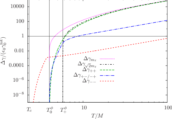
We show the temperature dependence of the C​P{C\!P}-asymmetries in neutrino decays in the full HTL calculation and in the one-mode approach for mℓm_{\ell} and 2​mℓ\sqrt{2}\,m_{\ell} in figure 11.

Refer to caption
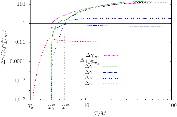
Figure 11: The C​P{C\!P}-asymmetries in neutrino decays normalised by the C​P{C\!P}-asymmetry in vacuum and the total decay density in vacuum, Δ​γ/(γ0tot​ϵ0)\Delta\gamma/(\gamma^{\rm tot}_{0}\epsilon_{0}). We choose M1=1010​GeVM_{1}=10^{10}\,{\rm GeV} and M2≫M1M_{2}\gg M_{1}. The term Δ​γh1​h2\Delta\gamma_{h_{1}h_{2}} denotes the difference between the decay rate and its C​P{C\!P} conjugated rate, which is proportional to the C​P{C\!P}-asymmetry. Here, h1h_{1} denotes the mode of the external lepton, while h2h_{2} denotes the mode of the lepton in the loop. For example, Δ​γ+⁣−=γ⁡(N→ϕ​ℓ+)−γ⁡(N→ϕ¯​ℓ¯+)\Delta\gamma_{+-}=\gamma(N\to\phi\ell_{+})-\gamma(N\to\bar{\phi}\bar{\ell}_{+}), where a minus-mode lepton is present in the loop. Δ​γmℓ\Delta\gamma_{m_{\ell}} and Δ​γ2​mℓ\Delta\gamma_{\sqrt{2}\,m_{\ell}} denote the rate differences for the one-mode approach with a thermal mass mℓm_{\ell} and an asymptotic thermal mass 2​mℓ\sqrt{2}\,m_{\ell}.

We choose M1=1010​GeVM_{1}=10^{10}{\rm\,GeV} and normalise the asymmetries by the product of the C​P{C\!P}-asymmetry at zero temperature and the total decay density in vacuum, ϵ0​γ0tot\epsilon_{0}\gamma_{0}^{\rm tot}. As discussed in sections 4.4 and 4.5, the vertex contribution and the self-energy contribution have the same temperature dependence for M2≫M1M_{2}\gg M_{1}. Moreover, as discussed in sections 4.4 and 4.5, the asymmetries are the same when we exchange the internal and the external lepton, therefore the asymmetry for a plus-mode external lepton combined with a minus-mode internal lepton is the same as the asymmetry for a minus-mode external lepton with a plus-mode internal lepton, in short, Δ​γ+⁣−=Δ​γ−⁣+\Delta\gamma_{+-}=\Delta\gamma_{-+}. We see that generally, the thresholds are the ones we expect from our analysis of the decay rates in section 3. For the one-mode calculations we have the expected thresholds at T0NT^{N}_{0} for mℓm_{\ell} and at T+NT^{N}_{+} for 2​mℓ\sqrt{2}\,m_{\ell}. For all asymmetries where a plus-mode lepton is involved, that is Δ​γ+⁣+\Delta\gamma_{++}, Δ​γ+⁣−\Delta\gamma_{+-} and Δ​γ−⁣+\Delta\gamma_{-+}, the phase space is reduced similar to the 2​mℓ\sqrt{2}\,m_{\ell} case below T+NT^{N}_{+} and an additional reduction of the phase space sets in between T+NT^{N}_{+} and T0NT^{N}_{0} since large momenta kk or k′k^{\prime} that correspond to a large mass m⁡(k)m(k) become kinematically forbidden. Between these two thresholds, T+NT_{+}^{N} and T0NT_{0}^{N}, the asymmetry for Δγ+−/−+\Delta\gamma_{+-/-+} becomes larger than the asymmetry for Δ​γ+⁣+\Delta\gamma_{++}. This effect occurs because in the (+⁣+++)-asymmetry the phase spaces of both the internal and the external lepton are suppressed, while for the mixed modes, (+⁣−+-) or (−⁣+-+), only the phase space of one momentum is suppressed, while the phase space of the other momentum is still large. The effect is similar to the observation that γ−\gamma_{-} becomes larger than γ+\gamma_{+} above T+NT_{+}^{N}. Relying solely on phase-space arguments, one would expect that Δ​γ2​mℓ\Delta\gamma_{\sqrt{2}\,m_{\ell}} is a good approximation for Δ​γ+⁣+\Delta\gamma_{++}. The fact that Δ​γ+⁣+\Delta\gamma_{++} is clearly smaller than Δ​γ2​mℓ\Delta\gamma_{\sqrt{2}\,m_{\ell}} is due to two suppressing factors: One factor is the effect of the two residues Zh​(k)Z_{h}(k) and Zh′​(k′)Z_{h^{\prime}}(k^{\prime}), which suppress the rate somewhat for small momenta kk and k′k^{\prime}. The other, more important factor is the fact that the helicity structure and angular dependence of the integrals are different for the (+⁣+++)- and the 2​mℓ\sqrt{2}\,m_{\ell}-case as explained in section 4.6. Since neutrino momenta are of the order ∼M1∼T\sim M_{1}\sim T for our temperature range, the lepton momenta will be of the same order, that is k>mℓk>m_{\ell}, and the leptons and Higgs bosons will preferentially be scattered forward. Thus also the angle ξ\xi between the two leptons will be small and the factor H−H_{-} defined in equation (106) is suppressed, while the corresponding one-mode factor 1−ξ⁡(k​k′)/(ωk​ωk′)1-\xi(kk^{\prime})/(\omega_{k}\omega_{k^{\prime}}) is larger than H−H_{-} for small angles and still finite if both leptons are scattered strictly in the same direction, that is ξ=1\xi=1. We have checked numerically that this is the main reason why Δ​γ2​mℓ>Δ​γ+⁣+\Delta\gamma_{\sqrt{2}\,m_{\ell}}>\Delta\gamma_{++} in the range 1/2​M1≲T≲T+N1/2\,M_{1}\lesssim T\lesssim T_{+}^{N}.

Since the C​P{C\!P}-asymmetries follow the corresponding finite-temperature decay rates that are shown in figure 5, it is very instructive to normalise them via these decay rates, that is γ+\gamma_{+}, γ−\gamma_{-}, γmℓ\gamma_{m_{\ell}} and γ2​mℓ\gamma_{\sqrt{2}\,m_{\ell}}. This also gives a more intuitive definition of the C​P{C\!P}-asymmetries at finite temperature. These asymmetries are shown in figure 12, normalised by the zero temperature C​P{C\!P}-asymmetry.

Refer to caption
Figure 12: The C​P{C\!P}-asymmetries in neutrino decays normalised by the C​P{C\!P}-asymmetry in vacuum and the corresponding total decay density at finite temperature, that is Δ​γ+⁣+/(γ+tot​ϵ0)\Delta\gamma_{++}/(\gamma^{\rm tot}_{+}\epsilon_{0}), Δ​γ−⁣+/(γ+tot​ϵ0)\Delta\gamma_{-+}/(\gamma^{\rm tot}_{+}\epsilon_{0}), Δ​γ+⁣−/(γ−tot​ϵ0)\Delta\gamma_{+-}/(\gamma^{\rm tot}_{-}\epsilon_{0}), Δ​γ−⁣−/(γ−tot​ϵ0)\Delta\gamma_{--}/(\gamma^{\rm tot}_{-}\epsilon_{0}), Δ​γmℓ/(γmℓtot​ϵ0)\Delta\gamma_{m_{\ell}}/(\gamma^{\rm tot}_{m_{\ell}}\epsilon_{0}) and Δ​γ2​mℓ/(γ2​mℓtot​ϵ0)\Delta\gamma_{\sqrt{2}\,m_{\ell}}/(\gamma^{\rm tot}_{\sqrt{2}\,m_{\ell}}\epsilon_{0}), where the C​P{C\!P} asymmetries Δ​γ\Delta\gamma are explained in figure 11. We choose M1=1010​GeVM_{1}=10^{10}\,{\rm GeV} and M2≫M1M_{2}\gg M_{1}.

Compared to the normalisation via γ0\gamma_{0} in figure 11, we see that the (+⁣+++)-asymmetry does not fall as steeply as the corresponding decay rate γ+\gamma_{+} between T+NT_{+}^{N} and T0NT_{0}^{N}, so the ratio Δ​γ+⁣+/γ+\Delta\gamma_{++}/\gamma_{+} is dented at the threshold T+NT_{+}^{N}. This illustrates that the (+⁣+++)-C​P{C\!P}-asymmetry shows a stronger suppression below the threshold T+NT_{+}^{N}, since it suffers from two phase space reductions and two residues that are smaller than one. Therefore, the (++)(++)-asymmetry is not affected as strongly as γ+\gamma_{+} by the additional suppression above T+NT_{+}^{N} when large momenta kk and k′k^{\prime} are forbidden and the transition over this threshold is smoother than for the decay rate γ+\gamma_{+}. So γ+\gamma_{+} falls more steeply than Δ​γ+⁣+\Delta\gamma_{++} above the threshold and the ratio of the two rates has a dent at T+NT_{+}^{N}. For the (+⁣−+-)-asymmetry, this effect is even stronger, since it is less suppressed than the (+⁣+++)-asymmetry above T+NT_{+}^{N}, so the ratio Δ​γ+⁣−/(ϵ0​γ−)\Delta\gamma_{+-}/(\epsilon_{0}\gamma_{-}) rises up to a value of 𝒪⁡(0.1)\mathcal{O}(0.1).

Refer to caption
Figure 13: The C​P{C\!P}-asymmetries in Higgs boson decays normalised by the C​P{C\!P}-asymmetry in vacuum and the total decay density in vacuum, Δ​γ/(γ0tot​ϵ0)\Delta\gamma/(\gamma^{\rm tot}_{0}\epsilon_{0}), where the asymmetries Δ​γ\Delta\gamma are explained in figure 11. We choose M1=1010​GeVM_{1}=10^{10}\,{\rm GeV} and M2≫M1M_{2}\gg M_{1}.
Refer to caption
Figure 14: The C​P{C\!P}-asymmetries in Higgs boson decays normalised by the C​P{C\!P}-asymmetry in vacuum and the corresponding total decay density at finite temperature, that is Δ​γ+⁣+/(γ+tot​ϵ0)\Delta\gamma_{++}/(\gamma^{\rm tot}_{+}\epsilon_{0}), Δ​γ−⁣+/(γ+tot​ϵ0)\Delta\gamma_{-+}/(\gamma^{\rm tot}_{+}\epsilon_{0}), Δ​γ+⁣−/(γ−tot​ϵ0)\Delta\gamma_{+-}/(\gamma^{\rm tot}_{-}\epsilon_{0}), Δ​γ−⁣−/(γ−tot​ϵ0)\Delta\gamma_{--}/(\gamma^{\rm tot}_{-}\epsilon_{0}), Δ​γmℓ/(γmℓtot​ϵ0)\Delta\gamma_{m_{\ell}}/(\gamma^{\rm tot}_{m_{\ell}}\epsilon_{0}) and Δ​γ2​mℓ/(γ2​mℓtot​ϵ0)\Delta\gamma_{\sqrt{2}\,m_{\ell}}/(\gamma^{\rm tot}_{\sqrt{2}\,m_{\ell}}\epsilon_{0}), where the C​P{C\!P} asymmetries Δ​γ\Delta\gamma are explained in figure 11. We choose M1=1010​GeVM_{1}=10^{10}\,{\rm GeV} and M2≫M1M_{2}\gg M_{1}.

The C​P{C\!P}-asymmetries in Higgs boson decays at high temperature are shown in figure 13, normalised to ϵ0​γtot\epsilon_{0}\gamma^{\rm tot} and we have assumed that M2≫M1,TM_{2}\gg M_{1},T. The behaviour is similar to the neutrino decays, where the (−⁣−--)-asymmetry is strongly suppressed, while the (+⁣−+-)-, the (−⁣+-+)- and the (+⁣+++)-asymmetries have a strict threshold at T0ϕT_{0}^{\phi} and are suppressed due to the reduced phase space between T0ϕT_{0}^{\phi} and T+ϕT_{+}^{\phi}, as expected. The (+⁣−+-)- and (−⁣+-+)- asymmetries are the same and are somewhat less suppressed than the (++)(++)-asymmetry between the thresholds T0ϕT_{0}^{\phi} and T+ϕT_{+}^{\phi}. In our approximation in section 4.6, we see that the difference of the matrix elements Δ​|ℳ|2\Delta|\mathcal{M}|^{2} rises as T2T^{2}, so Δ​γ\Delta\gamma rises as T4T^{4}, which can be seen in the plot for all finite-temperature asymmetries. The one-mode asymmetries Δ​γmℓ\Delta\gamma_{m_{\ell}}, Δ​γ2​mℓ\Delta\gamma_{\sqrt{2}\,m_{\ell}} and the (+⁣+++)-asymmetry are very close to each other at high temperature.

We also normalise the asymmetries to the corresponding decay rates in figure 14 and find that they all approach a constant value at high temperature, as is expected since the decay rates also rise as T4T^{4}. The dents in the ratios Δ​γ+⁣+/(ϵ0​γ+)\Delta\gamma_{++}/(\epsilon_{0}\gamma_{+}) and Δ​γ+⁣−/(ϵ0​γ+)\Delta\gamma_{+-}/(\epsilon_{0}\gamma_{+}) with an external plus-mode lepton are similar to the ones for the neutrino decays and due to the very strong suppression of γ+\gamma_{+} below the threshold T+ϕT_{+}^{\phi}. The numerically dominant asymmetries Δ​γmℓ\Delta\gamma_{m_{\ell}}, Δ​γ2​mℓ\Delta\gamma_{\sqrt{2}\,m_{\ell}} and Δ​γ+⁣+\Delta\gamma_{++} all settle at a rather high C​P{C\!P}-asymmetry, two orders of magnitude higher than at zero temperature, as we expect from our approximate calculation for a Higgs boson at rest in section 4.6. This is partly due to a suppression of |ℳ|2|\mathcal{M}|^{2} which rises as mϕ2=gϕ2​T2m_{\phi}^{2}=g_{\phi}^{2}T^{2}, but mainly due to the larger difference in matrix elements Δ​|ℳ|2\Delta|\mathcal{M}|^{2} for Higgs boson decays.

5 Conclusions

We have performed an extensive analysis of the effects of HTL corrections on C​PC\!P-asymmetries in neutrino and Higgs boson decays. This implies capturing the effects of thermal masses, modified dispersion relations and modified helicity structures. We put special emphasis on the influence of the two fermionic quasiparticles, which show a different behaviour than particles in vacuum, notably through their dispersion relations, but also the helicity structure of their interactions. Our work is thus similar to the work done in reference [14], where the authors of the latter work did not include the effects of fermionic quasiparticles and get a different result for the C​P{C\!P}-asymmetries, which are crucial for the evolution of the lepton asymmetry. We also approximate the lepton propagators by zero temperature propagators with the zero temperature mass replaced by the thermal lepton mass or the asymptotic mass. We refer to these cases as one-mode approach and compare the thermal cases to the zero-temperature case.

We have calculated HTL corrections to neutrino decays in reference [23] and shortly presented the Higgs decay rate at high temperature in reference [44], while we analyse this decay in detail in section 3. While the zero-temperature fermion mass vanishes in the unbroken electroweak phase, the resummation of HTL fermion self-energies results in an effective fermion propagator that does not break chiral invariance and is split up in two helicity modes. The external fermion states therefore behave conceptually different from the ones with chirality-breaking thermal masses that have been inserted in the kinematics by hand. Moreover, one has to take care of one additional mode, which has implications for the Boltzmann equations [22].

We calculated the C​P{C\!P}-asymmetries in section 4. To our knowledge, this is the first calculation of a C​P{C\!P}-asymmetry in leptogenesis that includes HTL-corrections and takes into account corrected thermal distributions for the particles in the loop.1313 13 Reference[14] has a calculation for the C​P{C\!P}-asymmetry of the neutrino and Higgs decays with HTL corrections in the propagators and thermal masses in the external states. They obtain a different combination of thermal distributions for the particles in the loop. The discrepancy is discussed in detail in reference[21]. The authors of the first reference get a factor 1−fℓ′+fϕ′−2​fℓ′​fϕ′1-f_{\ell^{\prime}}+f_{\phi^{\prime}}-2f_{\ell^{\prime}}f_{\phi^{\prime}} for the neutrino decays and fϕ′−fℓ′−2​fϕ′​fℓ′f_{\phi^{\prime}}-f_{\ell^{\prime}}-2f_{\phi^{\prime}}f_{\ell^{\prime}} for the Higgs boson decays due to an erroneous choice of cutting rules in the real time formalism. The correct calculation gives 1−fℓ′+fϕ′1-f_{\ell^{\prime}}+f_{\phi^{\prime}} for the neutrino decays and fϕ′+fℓ′f_{\phi^{\prime}}+f_{\ell^{\prime}} for the Higgs boson decays. This discrepancy is also responsible for our C​P{C\!P}-asymmetry in Higgs decays being a factor ten larger than their result. We present rules for the product of spinors that are related to the fermionic quasiparticles in equations (49) and (47) and derive frequency sums for the HTL fermion propagator in equation (99). We find four different C​P{C\!P}-asymmetries corresponding to the four different choices of lepton modes both in the loop and as external states. We find the C​P{C\!P}-asymmetry to be symmetric under an exchange of the lepton mode in the loop and the external lepton mode, such that Δ​γ+⁣−=Δ​γ−⁣+\Delta\gamma_{+-}=\Delta\gamma_{-+}. At finite temperature, there are three possible cuttings for the vertex contribution, the {ℓ′,ϕ′}\{\ell^{\prime},\phi^{\prime}\}-cut that corresponds to zero temperature and two additional cuts involving the internal N2N_{2}, namely through {N2,ℓ′}\{N_{2},\ell^{\prime}\} and {N′,ϕ′}\{N^{\prime},\phi^{\prime}\}, which have been found by references [14, 19, 45] and examined more closely in reference [20], using the real-time formalism. We obtain the same cuts using the imaginary time formalism and concentrate on the {ℓ′,ϕ′}\{\ell^{\prime},\phi^{\prime}\}-cut, assuming the hierarchical limit of M2≫M1M_{2}\gg M_{1}. As expected from the zero-temperature result, we find the vertex contribution proportional to the self-energy contribution in this limit. Contrary to reference [14], we find that the C​P{C\!P}-asymmetry in Higgs boson decays is larger than the asymmetry in neutrino decays by about a factor of 100100 if appropriately normalised. This is due to a suppression of the Higgs boson decay rate and a thermal enhancement of the C​P{C\!P}-asymmetry by the distribution functions of the Higgs bosons and leptons. We compare the C​P{C\!P}-asymmetries in the two-mode approach to the C​P{C\!P}-asymmetries in the one-mode approach. We find that for the two-mode approach, the helicity structure of the modes prohibits the two leptons to be scattered strictly in the same direction while for the one-mode approach, this direction is only mildly suppressed. Notably this fact is responsible for suppressing the (+⁣+++)-C​P{C\!P}-asymmetry compared to the asymmetries of the one-mode approach, as well as the residues of the plus-modes to less extent.

Summarising, we argue that for an accurate description of medium effects on leptogenesis, the influence of thermal quasiparticles, notably the effects of the two fermionic modes, cannot be neglected. The corresponding C​PC\!P-asymmetries show a considerable deviation from the one-mode asymmetries in the interesting temperature regime T∼M1T\sim M_{1}. Moreover, the presence of a new minus-mode that essentially does not interact with the SM turns out to have implications for the lepton asymmetry even in the strong washout regime, as we found in an additional study [22].

Acknowledgements

We would like to thank Mathias Garny, Georg Raffelt, Michael A. Schmidt and Markus Thoma for their support and comments in this project. Thanks also to Denis Besak, Dietrich Bödeker, Wilfried Buchmüller, Valerie Domcke, Marco Drewes, Andreas Hohenegger, Alexander Kartavtsev and Christoph Weniger for fruitful and inspiring discussions.

Appendix A Frequency Sums

A.1 Frequency sums for HTL fermion propagators

In order to deal with the HTL lepton propagator, we derive frequency sums for the propagator parts Δ±​(K)\Delta_{\pm}(K) of a fermion propagator. We write the propagator in the Saclay representation as

Δ~h​(K)\displaystyle\tilde{\Delta}_{h}(K) =−∫0βdτek0​τΔ~h(τ,𝐤),\displaystyle=-\int_{0}^{\beta}{\rm d}\tau\,{\rm e}^{k_{0}\tau}\tilde{\Delta}_{h}(\tau,{\bf k})\,,
Δ~h​(τ,𝐤)\displaystyle\tilde{\Delta}_{h}(\tau,{\bf k}) =∫−∞∞d​ω​ρh​fF​(−ω)​e−ω​τ,\displaystyle=\int_{-\infty}^{\infty}{\rm d}\omega\,\rho_{h}f_{F}(-\omega){\rm e}^{-\omega\tau}\,, (94)

where fFf_{F} stands for a Fermi-Dirac distribution. Since we are only interested in the pole contribution, we write the corresponding spectral density as

ρhpole\displaystyle\rho_{h}^{\rm pole} =−Zh[δ(ω−ωh)+δ(ω+ω−h)]=−∑sZs​hδ(ω−sωs​h),\displaystyle=-Z_{h}[\delta(\omega-\omega_{h})+\delta(\omega+\omega_{-h})]=-\sum_{s}Z_{sh}\delta(\omega-s\omega_{sh})\,, (95)

where s​hsh in Zs​hZ_{sh} and ωs​h\omega_{sh} denotes the product of ss and hh, that is, Zs​h=Z+Z_{sh}=Z_{+} for s=h=−1s=h=-1 for example. We have for the propagator

Δ~hpole​(τ,𝐤)\displaystyle\tilde{\Delta}_{h}^{\rm pole}(\tau,{\bf k}) =−∫−∞∞dω∑sZs​hδ(ω−sωs​h)fF(−ω)e−ω​τ\displaystyle=-\int_{-\infty}^{\infty}{\rm d}\omega\,\sum_{s}Z_{sh}\delta(\omega-s\omega_{sh})f_{F}(-\omega){\rm e}^{-\omega\tau}
=−∑sZs​hfF(−sωs​h)e−s​ωs​h​τ=∑sΔ~h,spole(τ,𝐤),\displaystyle=-\sum_{s}Z_{sh}f_{F}(-s\omega_{sh}){\rm e}^{-s\omega_{sh}\tau}=\sum_{s}\tilde{\Delta}_{h,s}^{\rm pole}(\tau,{\bf k}),
Δ~hpole​(K)\displaystyle\tilde{\Delta}_{h}^{\rm pole}(K) =∑sZs​h​fF​(−s​ωs​h)​∫0βd​τ​e(k0−s​ωs​h)​τ=∑sΔ~h,spole​(K),\displaystyle=\sum_{s}Z_{sh}f_{F}(-s\omega_{sh})\int_{0}^{\beta}{\rm d}\tau\,{\rm e}^{(k_{0}-s\omega_{sh})\tau}=\sum_{s}\tilde{\Delta}^{\rm pole}_{h,s}(K)\,,
Δ~h,spole​(K)\displaystyle\tilde{\Delta}_{h,s}^{\rm pole}(K) =Zs​h​fF​(−s​ωs​h)​∫0βd​τ​e(k0−s​ωs​h)​τ\displaystyle=Z_{sh}f_{F}(-s\omega_{sh})\int_{0}^{\beta}{\rm d}\tau\,{\rm e}^{(k_{0}-s\omega_{sh})\tau}
=−Zs​h​1k0−s​ωs​h,\displaystyle=-Z_{sh}\frac{1}{k_{0}-s\omega_{sh}}\,, (96)

where Zs​h=(ωs​h2−k2)/(2​mℓ2)Z_{sh}=(\omega_{sh}^{2}-k^{2})/(2m_{\ell}^{2}) is the quasiparticle residuum.

In dealing with frequency sums of bare thermal propagators, it is very convenient to write

Δs​(K)=Δ−s​(−K).\displaystyle\Delta_{s}(K)=\Delta_{-s}(-K). (97)

Replacing a boson by a fermion amounts to replacing fB​(ω)f_{B}(\omega) by −fF​(ω)-f_{F}(\omega). Moreover, calculating a frequency sum of k0k_{0} times the propagators amounts to replacing k0k_{0} with s​ωs\omega as in

T​∑k0k0​Δs1​(K)​Δs2​(P−K)=s1​ω​T​∑k0Δs1​(K)​Δs2​(P−K),\displaystyle T\sum_{k_{0}}k_{0}\Delta_{s_{1}}(K)\Delta_{s_{2}}(P-K)=s_{1}\omega T\sum_{k_{0}}\Delta_{s_{1}}(K)\Delta_{s_{2}}(P-K), (98)

where ω=k2+m2\omega=\sqrt{k^{2}+m^{2}} and mm is the mass of the first boson. The same holds for fermions.

It is straightforward to work out the frequency sums for the resummed lepton propagator,

T​∑k0Δ~h,s1pole​(k0,ω)​Δs2​(p0−k0,ω)=Zs1​h​s22​ω​1−fF​(s1​ωs1​h)+fB​(s2​ω)p0−s1​ωs1​h−s2​ω,\displaystyle T\sum_{k_{0}}\tilde{\Delta}_{h,s_{1}}^{\rm pole}(k_{0},\omega)\Delta_{s_{2}}(p_{0}-k_{0},\omega)=Z_{s_{1}h}\frac{s_{2}}{2\omega}\frac{1-f_{F}(s_{1}\omega_{s_{1}h})+f_{B}(s_{2}\omega)}{p_{0}-s_{1}\omega_{s_{1}h}-s_{2}\omega}, (99)

where the other necessary frequency sums can be derived from this by making the appropriate substitutions.

A.2 The frequency sum for the vertex contribution

The frequency sums for the pole part of a HTL fermion propagator is derived in appendix A.1. We calculate the frequency sum of the three propagators in the vertex loop by partial fractioning

Δ~s,h′pole​Δsϕ′​Δ~sN′=Cs​ϕ​N′​[sϕ′2​ωϕ′​Δ~s,h′pole​Δ~sN′−sN′2​ωN′​Δ~s,h′pole​Δsϕ′].\displaystyle\tilde{\Delta}_{s,h^{\prime}}^{\rm pole}\Delta_{s_{\phi^{\prime}}}\tilde{\Delta}_{s_{N^{\prime}}}=C_{s\phi N^{\prime}}\left[\frac{s_{\phi^{\prime}}}{2\omega_{\phi^{\prime}}}\tilde{\Delta}_{s,h^{\prime}}^{\rm pole}\tilde{\Delta}_{s_{N^{\prime}}}-\frac{s_{N^{\prime}}}{2\omega_{N^{\prime}}}\tilde{\Delta}_{s,h^{\prime}}^{\rm pole}\Delta_{s_{\phi^{\prime}}}\right]\,. (100)

We are using ΔN′​(P′)=ΔN′​(−P′)\Delta_{N^{\prime}}(P^{\prime})=\Delta_{N^{\prime}}(-P^{\prime}) and

Cs​ϕ​N′=1k0−sϕ′​ωϕ′+sN′​ωN′.\displaystyle C_{s\phi N^{\prime}}=\frac{1}{k_{0}-s_{\phi^{\prime}}\omega_{\phi^{\prime}}+s_{N^{\prime}}\omega_{N^{\prime}}}. (101)

The frequency sum is given by

T​∑k0′Δ~s,h′pole​Δsϕ′​Δ~sN′=Zs​h′​sϕ′​sN′4​ωϕ′​ωN′​Cs​ϕ​N′​[Zs​h​N′Ns​h​N′−Zs​h​ϕ′Ns​h​ϕ′],\displaystyle T\sum_{k_{0}^{\prime}}\tilde{\Delta}_{s,h^{\prime}}^{\rm pole}\Delta_{s_{\phi^{\prime}}}\tilde{\Delta}_{s_{N^{\prime}}}=Z_{sh^{\prime}}\frac{s_{\phi^{\prime}}s_{N^{\prime}}}{4\omega_{\phi^{\prime}}\omega_{N^{\prime}}}C_{s\phi N^{\prime}}\left[\frac{Z_{shN^{\prime}}}{N_{shN^{\prime}}}-\frac{Z_{sh\phi^{\prime}}}{N_{sh\phi^{\prime}}}\right], (102)

where

Zs​h​N′\displaystyle Z_{shN^{\prime}} =1−fF​(s​ωs​h′)−fF​(sN′​ωN′),\displaystyle=1-f_{F}(s\omega_{sh^{\prime}})-f_{F}(s_{N^{\prime}}\omega_{N^{\prime}})\,,
Zs​h​ϕ′\displaystyle Z_{sh\phi^{\prime}} =1−fF​(s​ωs​h′)+f⁡(sϕ′​ωϕ′),\displaystyle=1-f_{F}(s\omega_{sh^{\prime}})+f(s_{\phi^{\prime}}\omega_{\phi^{\prime}})\,, (103)

and

Ns​h​N′\displaystyle N_{shN^{\prime}} =q0−s​ωs​h′−sN′​ωN′,\displaystyle=q_{0}-s\omega_{sh^{\prime}}-s_{N^{\prime}}\omega_{N^{\prime}}\,,
Ns​h​ϕ′\displaystyle N_{sh\phi^{\prime}} =p0−s​ωs​h′−sϕ′​ωϕ′.\displaystyle=p_{0}-s\omega_{sh^{\prime}}-s_{\phi^{\prime}}\omega_{\phi^{\prime}}\,. (104)

Summing over all propagator parts and the helicity-over-chirality ratios, we get

T​∑k0′∑h′ΔN′​Δϕ′​Δ′​H−=∑h′Zh′4​ωq′​ωp′​{E−​H−+E+​H+},\displaystyle T\sum_{k_{0}^{\prime}}\sum_{h^{\prime}}\Delta_{N^{\prime}}\Delta_{\phi^{\prime}}\Delta^{\prime}H_{-}=\sum_{h^{\prime}}\frac{Z_{h^{\prime}}}{4\omega_{q^{\prime}}\omega_{p^{\prime}}}\left\{E_{-}H_{-}+E_{+}H_{+}\right\}, (105)

where

H±\displaystyle H_{\pm} =1±h​h′​ξ,\displaystyle=1\pm hh^{\prime}\xi\,,
ξ\displaystyle\xi =𝐤^⋅𝐤′^.\displaystyle=\bf{\hat{k}\cdot\hat{k^{\prime}}}\,. (106)

The coefficients E±E_{\pm} are given by

E−\displaystyle E_{-} =Fϕ​N​Aℓϕ′−Fℓ′​N​Aℓℓ−Fϕ​ℓ′​Aℓ0+Fℓ′​ℓ′​AℓN′,\displaystyle=F^{\phi N}A_{\ell}^{\phi^{\prime}}-F^{\ell^{\prime}N}A_{\ell}^{\ell}-F^{\phi\ell^{\prime}}A_{\ell}^{0}+F^{\ell^{\prime}\ell^{\prime}}A_{\ell}^{N^{\prime}}, (107)
E+\displaystyle E_{+} =FN′​ϕ′​Aℓϕ′−F0​ϕ′​Aℓℓ−FN′​0​Aℓ0+F00​AℓN′,\displaystyle=F^{N^{\prime}\phi^{\prime}}A_{\ell}^{\phi^{\prime}}-F^{0\phi^{\prime}}A_{\ell}^{\ell}-F^{N^{\prime}0}A_{\ell}^{0}+F^{00}A_{\ell}^{N^{\prime}}, (108)

and the coefficients Fi​jF^{ij} read

Fϕ​N\displaystyle F^{\phi N} =Bϕϕ−BNN,\displaystyle=B_{\phi}^{\phi}-B_{N}^{N}, FN′​ϕ′\displaystyle F^{N^{\prime}\phi^{\prime}} =BϕN′−BNϕ′,\displaystyle=B_{\phi}^{N^{\prime}}-B_{N}^{\phi^{\prime}},
Fℓ′​N\displaystyle F^{\ell^{\prime}N} =Bϕℓ′−BNN,\displaystyle=B_{\phi}^{\ell^{\prime}}-B_{N}^{N}, F0​ϕ′\displaystyle F^{0\phi^{\prime}} =Bϕ0−BNϕ′,\displaystyle=B_{\phi}^{0}-B_{N}^{\phi^{\prime}},
Fϕ​ℓ′\displaystyle F^{\phi\ell^{\prime}} =Bϕϕ−BNℓ′,\displaystyle=B_{\phi}^{\phi}-B_{N}^{\ell^{\prime}}, FN′​0\displaystyle F^{N^{\prime}0} =BϕN′−BN0,\displaystyle=B_{\phi}^{N^{\prime}}-B_{N}^{0},
Fℓ′​ℓ′\displaystyle F^{\ell^{\prime}\ell^{\prime}} =Bϕℓ′−BNℓ′,\displaystyle=B_{\phi}^{\ell^{\prime}}-B_{N}^{\ell^{\prime}}, F00\displaystyle F^{00} =Bϕ0−BN0.\displaystyle=B_{\phi}^{0}-B_{N}^{0}. (109)

The factors BN/ϕB_{N/\phi} and AℓA_{\ell} are given by

BN/ϕψ=\displaystyle B_{N/\phi}^{\psi}= ZN/ϕψNN/ϕψ,\displaystyle\frac{Z_{N/\phi}^{\psi}}{N_{N/\phi}^{\psi}}\,, Aℓψ=\displaystyle A_{\ell}^{\psi}= 1Nℓψ,\displaystyle\frac{1}{N_{\ell}^{\psi}}\,, (110)

where the numerators and denominators read

NNN\displaystyle N_{N}^{N} =p0−ω′−ωq′,\displaystyle=p_{0}-\omega^{\prime}-\omega_{q^{\prime}}, Nℓℓ\displaystyle N_{\ell}^{\ell} =k0−ωq′−ωp′,\displaystyle=k_{0}-\omega_{q^{\prime}}-\omega_{p^{\prime}}, Nϕϕ\displaystyle N_{\phi}^{\phi} =q0−ω′−ωp′,\displaystyle=q_{0}-\omega^{\prime}-\omega_{p^{\prime}},
NN0\displaystyle N_{N}^{0} =p0+ω′+ωq′,\displaystyle=p_{0}+\omega^{\prime}+\omega_{q^{\prime}}, Nℓ0\displaystyle N_{\ell}^{0} =k0+ωq′+ωp′,\displaystyle=k_{0}+\omega_{q^{\prime}}+\omega_{p^{\prime}}, Nϕ0\displaystyle N_{\phi}^{0} =q0+ω′+ωp′,\displaystyle=q_{0}+\omega^{\prime}+\omega_{p^{\prime}},
NNℓ′\displaystyle N_{N}^{\ell^{\prime}} =p0−ω′+ωq′,\displaystyle=p_{0}-\omega^{\prime}+\omega_{q^{\prime}}, Nℓϕ′\displaystyle N_{\ell}^{\phi^{\prime}} =k0−ωq′+ωp′,\displaystyle=k_{0}-\omega_{q^{\prime}}+\omega_{p^{\prime}}, Nϕℓ′\displaystyle N_{\phi}^{\ell^{\prime}} =q0−ω′+ωp′,\displaystyle=q_{0}-\omega^{\prime}+\omega_{p^{\prime}},
NNϕ′\displaystyle N_{N}^{\phi^{\prime}} =p0+ω′−ωq′,\displaystyle=p_{0}+\omega^{\prime}-\omega_{q^{\prime}}, NℓN′\displaystyle N_{\ell}^{N^{\prime}} =k0+ωq′−ωp′,\displaystyle=k_{0}+\omega_{q^{\prime}}-\omega_{p^{\prime}}, NϕN′\displaystyle N_{\phi}^{N^{\prime}} =q0+ω′−ωp′,\displaystyle=q_{0}+\omega^{\prime}-\omega_{p^{\prime}}\,, (111)

and

ZNN\displaystyle Z_{N}^{N} =1−fℓ′+fϕ′,\displaystyle=1-f_{\ell^{\prime}}+f_{\phi^{\prime}}\,, Zϕϕ\displaystyle Z_{\phi}^{\phi} =1−fℓ′−fN′,\displaystyle=1-f_{\ell^{\prime}}-f_{N^{\prime}}\,,
ZN0\displaystyle Z_{N}^{0} =−(1−fℓ′+fϕ′),\displaystyle=-(1-f_{\ell^{\prime}}+f_{\phi^{\prime}})\,, Zϕ0\displaystyle Z_{\phi}^{0} =−(1−fℓ′−fN′),\displaystyle=-(1-f_{\ell^{\prime}}-f_{N^{\prime}})\,,
ZNℓ′\displaystyle Z_{N}^{\ell^{\prime}} =−(fℓ′+fϕ′),\displaystyle=-(f_{\ell^{\prime}}+f_{\phi^{\prime}})\,, Zϕℓ′\displaystyle Z_{\phi}^{\ell^{\prime}} =−(fℓ′−fN′),\displaystyle=-(f_{\ell^{\prime}}-f_{N^{\prime}})\,,
ZNϕ′\displaystyle Z_{N}^{\phi^{\prime}} =fℓ′+fϕ′,\displaystyle=f_{\ell^{\prime}}+f_{\phi^{\prime}}\,, ZϕN′\displaystyle Z_{\phi}^{N^{\prime}} =fℓ′−fN′.\displaystyle=f_{\ell^{\prime}}-f_{N^{\prime}}\,. (112)

We can write

T​∑k0′∑h′ΔN′​Δϕ′​Δh′​H−=∑h′Zh′4​ωq′​ωp′{[Fϕ​NAℓϕ′−Fℓ′​NAℓℓ−Fϕ​ℓ′Aℓ0+Fℓ′​ℓ′AℓN′]H−+[FN′​ϕ′Aℓϕ′−F0​ϕ′Aℓℓ−FN′​0Aℓ0+F00AℓN′]H+}\displaystyle\begin{split}T\sum_{k_{0}^{\prime}}\sum_{h^{\prime}}\Delta_{N^{\prime}}\Delta_{\phi^{\prime}}\Delta_{h^{\prime}}H_{-}=\sum_{h^{\prime}}\frac{Z_{h^{\prime}}}{4\omega_{q^{\prime}}\omega_{p^{\prime}}}&\left\{\left[F^{\phi N}A_{\ell}^{\phi^{\prime}}-F^{\ell^{\prime}N}A_{\ell}^{\ell}-F^{\phi\ell^{\prime}}A_{\ell}^{0}+F^{\ell^{\prime}\ell^{\prime}}A_{\ell}^{N^{\prime}}\right]H_{-}\right.\\ &\hskip-6.0pt+\left.\left[F^{N^{\prime}\phi^{\prime}}A_{\ell}^{\phi^{\prime}}-F^{0\phi^{\prime}}A_{\ell}^{\ell}-F^{N^{\prime}0}A_{\ell}^{0}+F^{00}A_{\ell}^{N^{\prime}}\right]H_{+}\right\}\end{split} (113)

or, more explicitly,

T∑k0′∑h′ΔN′​Δϕ′​Δh′​H−==∑h′Zh′4​ωq′​ωp′{[(Bϕϕ−BNN)Aℓϕ′−(Bϕℓ′−BNN)Aℓℓ−(Bϕϕ−BNℓ′)Aℓ0+(Bϕℓ′−BNℓ′)AℓN′]H−+[(BϕN′−BNϕ′)Aℓϕ′−(Bϕ0−BNϕ′)Aℓℓ−(BϕN′−BN0)Aℓ0+(Bϕ0−BN0)AℓN′]H+}.\displaystyle\begin{split}T\sum_{k_{0}^{\prime}}\sum_{h^{\prime}}&\Delta_{N^{\prime}}\Delta_{\phi^{\prime}}\Delta_{h^{\prime}}H_{-}=\\ =\sum_{h^{\prime}}\frac{Z_{h^{\prime}}}{4\omega_{q^{\prime}}\omega_{p^{\prime}}}&\left\{\left[\left(B_{\phi}^{\phi}-B_{N}^{N}\right)A_{\ell}^{\phi^{\prime}}-\left(B_{\phi}^{\ell^{\prime}}-B_{N}^{N}\right)A_{\ell}^{\ell}-\left(B_{\phi}^{\phi}-B_{N}^{\ell^{\prime}}\right)A_{\ell}^{0}+\left(B_{\phi}^{\ell^{\prime}}-B_{N}^{\ell^{\prime}}\right)A_{\ell}^{N^{\prime}}\right]H_{-}\right.\\ &\hskip-6.0pt+\left.\left[\left(B_{\phi}^{N^{\prime}}-B_{N}^{\phi^{\prime}}\right)A_{\ell}^{\phi^{\prime}}-\left(B_{\phi}^{0}-B_{N}^{\phi^{\prime}}\right)A_{\ell}^{\ell}-\left(B_{\phi}^{N^{\prime}}-B_{N}^{0}\right)A_{\ell}^{0}+\left(B_{\phi}^{0}-B_{N}^{0}\right)A_{\ell}^{N^{\prime}}\right]H_{+}\right\}\,.\end{split} (114)

Appendix B Analytic Expressions for the 𝑪​𝑷\boldsymbol{C\!P}-Asymmetries

B.1 Vertex cut through {ℓ′,ϕ′}\boldsymbol{\{\ell^{\prime},\phi^{\prime}\}}

We simplify the analytic expression for ϵγ​(T)\epsilon_{\gamma}(T) in equation (35). For IVI_{V} in equation (53) we get

Im​(IV)NNN=M1​M216​π2​Zh​ωp​∑h′∫0∞d​k′​∫0πd​ϕ′​k′ωp′​Zh′​ZNN​(Aℓℓ−Aℓϕ′)​H−,\displaystyle{\rm Im}(I_{V})_{N_{N}^{N}}=\frac{M_{1}M_{2}}{16\pi^{2}}\frac{Z_{h}\omega}{p}\sum_{h^{\prime}}\int_{0}^{\infty}{\rm d}k^{\prime}\int_{0}^{\pi}{\rm d}\phi^{\prime}\frac{k^{\prime}}{\omega_{p^{\prime}}}Z_{h^{\prime}}Z_{N}^{N}(A_{\ell}^{\ell}-A_{\ell}^{\phi^{\prime}})H_{-}, (115)

where it is sufficient to integrate ϕ′\phi^{\prime} from 00 to π\pi. The difference of the matrix elements reads for the vertex contribution

|ℳ⁡(N→ℓh​ϕ)|2−|ℳ⁡(N→ℓ¯h​ϕ¯)|2=\displaystyle\left|\mathcal{M}(N\to\ell_{h}\phi)\right|^{2}-\left|\mathcal{M}(N\to\bar{\ell}_{h}\bar{\phi})\right|^{2}= −gS​U​(2)​Im​{[(λ†​λ)12]2}​M1​M24​π2​Zh​ωhp\displaystyle-g_{SU(2)}{\rm Im}\left\{\left[\left(\lambda^{\dagger}\lambda\right)_{12}\right]^{2}\right\}\frac{M_{1}M_{2}}{4\pi^{2}}\frac{Z_{h}\omega_{h}}{p}
×∑h′∫0∞d​k′​∫0πd​ϕ′​k′ωp′​Zh′​ZNN​(Aℓℓ−Aℓϕ′)​H−.\displaystyle\times\sum_{h^{\prime}}\int_{0}^{\infty}{\rm d}k^{\prime}\int_{0}^{\pi}{\rm d}\phi^{\prime}\frac{k^{\prime}}{\omega_{p^{\prime}}}Z_{h^{\prime}}Z_{N}^{N}(A_{\ell}^{\ell}-A_{\ell}^{\phi^{\prime}})H_{-}\,. (116)

Correspondingly, the difference in decay rates reads

γ⁡(N→ℓh​ϕ)−γ⁡(N→ℓ¯h​ϕ¯)=\displaystyle\gamma(N\to\ell_{h}\phi)-\gamma(N\to\bar{\ell}_{h}\bar{\phi})= −gS​U​(2)​Im​{[(λ†​λ)12]2}​M1​M24​(2​π)5\displaystyle-g_{SU(2)}{\rm Im}\left\{\left[\left(\lambda^{\dagger}\lambda\right)_{12}\right]^{2}\right\}\frac{M_{1}M_{2}}{4(2\pi)^{5}}
×∑h′∫d​E​𝑑k​d​k′​∫0πd​ϕ′​k​FN​h​Zh​k′p​ωp′​ZNN​Zh′​(Aℓℓ−Aℓϕ′)​H−,\displaystyle\times\sum_{h^{\prime}}\int{\rm d}E{\rm d}k{\rm d}k^{\prime}\int_{0}^{\pi}{\rm d}\phi^{\prime}kF_{Nh}Z_{h}\frac{k^{\prime}}{p\omega_{p^{\prime}}}Z_{N}^{N}Z_{h^{\prime}}(A_{\ell}^{\ell}-A_{\ell}^{\phi^{\prime}})H_{-}\,, (117)

where FN​h=fNeq​(1+fϕeq)​(1−fℓ​heq)F_{Nh}=f_{N}^{\rm eq}(1+f_{\phi}^{\rm eq})(1-f_{\ell h}^{\rm eq}) is the statistical factor for the decay.

We know from section 3 that

∑s|ℳhs​(N→L​H)|2=gS​U​(2)​gc​(λ†​λ)11​Zh​ω​(p0−h​p​η),\displaystyle\sum_{s}\left|\mathcal{M}^{s}_{h}(N\to LH)\right|^{2}=g_{SU(2)}g_{c}(\lambda^{\dagger}\lambda)_{11}Z_{h}\omega(p_{0}-hp\eta)\,, (118)

where gc=2g_{c}=2 indicates that we sum over N→ϕ​ℓN\to\phi\ell and N→ϕ¯​ℓ¯N\to\bar{\phi}\bar{\ell}. Thus

Γ⁡(N→Lh​H)=gS​U​(2)​gc​(λ†​λ)1116​π​p​p0​∫d​k​k​ZD​Zh​(p0−h​p​η)\displaystyle\Gamma(N\to L_{h}H)=g_{SU(2)}g_{c}\frac{(\lambda^{\dagger}\lambda)_{11}}{16\pi pp_{0}}\int{\rm d}kkZ_{D}Z_{h}(p_{0}-hp\eta) (119)

and

γ⁡(N→Lh​H)=gS​U​(2)​gc​(λ†​λ)114​(2​π)3​∫d​E​𝑑k​k​fN​ZD​Zh​(p0−h​p​η),\displaystyle\gamma(N\to L_{h}H)=g_{SU(2)}g_{c}\frac{(\lambda^{\dagger}\lambda)_{11}}{4(2\pi)^{3}}\int{\rm d}E{\rm d}kkf_{N}Z_{D}Z_{h}(p_{0}-hp\eta)\,, (120)

where we have summed over the neutrino degrees of freedom.

We arrive at

ϵh​(T)=\displaystyle\epsilon_{h}(T)= −gS​U​(2)Im⁡{[(λ†​λ)12]2}γ⁡(N→Lh​N)M1​M24​(2​π)5∑h′∫dEdkdk′∫0πdϕ′kFNheqZhk′p​ωp′ZNNZh′(Aℓℓ−Aℓϕ′)H−\displaystyle-g_{SU(2)}\frac{{\rm Im}\{[(\lambda^{\dagger}\lambda)_{12}]^{2}\}}{\gamma(N\to L_{h}N)}\frac{M_{1}M_{2}}{4(2\pi)^{5}}\sum_{h^{\prime}}\int{\rm d}E{\rm d}k{\rm d}k^{\prime}\int_{0}^{\pi}{\rm d}\phi^{\prime}kF_{N_{h}}^{\rm eq}Z_{h}\frac{k^{\prime}}{p\omega_{p^{\prime}}}Z_{N}^{N}Z_{h^{\prime}}(A_{\ell}^{\ell}-A_{\ell}^{\phi^{\prime}})H_{-}
=\displaystyle= −Im⁡{[(λ†​λ)12]2}gc​(λ†​λ)11​M1​M24​π2​∑h′∫d​E​𝑑k​d​k′​∫0πd​ϕ′​k​FNheq​Zh​k′p​ωp′​ZNN​Zh′​(Aℓℓ−Aℓϕ′)​H−∫d​E​𝑑k​k​fN​ZD​Zh​(p0−h​p​η).\displaystyle-\frac{{\rm Im}\{[(\lambda^{\dagger}\lambda)_{12}]^{2}\}}{g_{c}(\lambda^{\dagger}\lambda)_{11}}\frac{M_{1}M_{2}}{4\pi^{2}}\frac{\sum_{h^{\prime}}\int{\rm d}E{\rm d}k{\rm d}k^{\prime}\int_{0}^{\pi}{\rm d}\phi^{\prime}kF_{N_{h}}^{\rm eq}Z_{h}\frac{k^{\prime}}{p\omega_{p^{\prime}}}Z_{N}^{N}Z_{h^{\prime}}(A_{\ell}^{\ell}-A_{\ell}^{\phi^{\prime}})H_{-}}{\int{\rm d}E{\rm d}kkf_{N}Z_{D}Z_{h}(p_{0}-hp\eta)}\,. (121)

B.2 Self-energy cut

For the self-energy contribution, we get

Im​(IS)NN=M1​M2M12−M22​14​π2​Zh​ωp​∑h​h′∫0∞d​k′​∫0πd​ϕ′​k′​Zh′​ZNN​H−.\displaystyle{\rm Im}(I_{S})_{N_{N}}=\frac{M_{1}M_{2}}{M_{1}^{2}-M_{2}^{2}}\frac{1}{4\pi^{2}}\frac{Z_{h}\omega}{p}\sum_{hh^{\prime}}\int_{0}^{\infty}{\rm d}k^{\prime}\int_{0}^{\pi}{\rm d}\phi^{\prime}k^{\prime}Z_{h^{\prime}}Z_{N}^{N}H_{-}\,. (122)

The difference in decay rates reads

γ⁡(N→ℓh​ϕ)−γ⁡(N→ℓ¯h​ϕ¯)=\displaystyle\gamma(N\to\ell_{h}\phi)-\gamma(N\to\bar{\ell}_{h}\bar{\phi})= −gS​U​(2)​Im​{[(λ†​λ)12]2}​M1​M2(M12−M22)​1(2​π)5\displaystyle-g_{SU(2)}{\rm Im}\left\{\left[\left(\lambda^{\dagger}\lambda\right)_{12}\right]^{2}\right\}\frac{M_{1}M_{2}}{(M_{1}^{2}-M_{2}^{2})}\frac{1}{(2\pi)^{5}}
×∑h′∫d​E​𝑑k​d​k′​∫0πd​ϕ′​k​FNheq​Zh​k′p​ZNN​Zh′​H−.\displaystyle\times\sum_{h^{\prime}}\int{\rm d}E{\rm d}k{\rm d}k^{\prime}\int_{0}^{\pi}{\rm d}\phi^{\prime}kF_{N_{h}}^{\rm eq}Z_{h}\frac{k^{\prime}}{p}Z_{N}^{N}Z_{h^{\prime}}H_{-}\,. (123)

The C​P{C\!P}-asymmetry reads

ϵh​(T)=\displaystyle\epsilon_{h}(T)= −gS​U​(2)Im⁡{[(λ†​λ)12]2}γ⁡(N→Lh​N)M1​M2M12−M221(2​π)5∑h′∫dEdkdk′∫0πdϕ′kFNheqZhk′pZNNZh′H−\displaystyle-g_{SU(2)}\frac{{\rm Im}\{[(\lambda^{\dagger}\lambda)_{12}]^{2}\}}{\gamma(N\to L_{h}N)}\frac{M_{1}M_{2}}{M_{1}^{2}-M_{2}^{2}}\frac{1}{(2\pi)^{5}}\sum_{h^{\prime}}\int{\rm d}E{\rm d}k{\rm d}k^{\prime}\int_{0}^{\pi}{\rm d}\phi^{\prime}kF_{N_{h}}^{\rm eq}Z_{h}\frac{k^{\prime}}{p}Z_{N}^{N}Z_{h^{\prime}}H_{-}
=\displaystyle= −Im⁡{[(λ†​λ)12]2}gc​(λ†​λ)11​M1​M2M12−M22​12​π2​∑h′∫d​E​𝑑k​d​k′​∫0πd​ϕ′​k​FNheq​Zh​k′p​ZNN​Zh′​H−∫d​E​𝑑k​k​fN​ZD​Zh​(p0−h​p​η),\displaystyle-\frac{{\rm Im}\{[(\lambda^{\dagger}\lambda)_{12}]^{2}\}}{g_{c}(\lambda^{\dagger}\lambda)_{11}}\frac{M_{1}M_{2}}{M_{1}^{2}-M_{2}^{2}}\frac{1}{2\pi^{2}}\frac{\sum_{h^{\prime}}\int{\rm d}E{\rm d}k{\rm d}k^{\prime}\int_{0}^{\pi}{\rm d}\phi^{\prime}kF_{N_{h}}^{\rm eq}Z_{h}\frac{k^{\prime}}{p}Z_{N}^{N}Z_{h^{\prime}}H_{-}}{\int{\rm d}E{\rm d}kkf_{N}Z_{D}Z_{h}(p_{0}-hp\eta)}\,, (124)

Appendix C The Other Cuts

C.1 Imaginary Parts

Vertex cut through {𝑵𝟐,ϕ′}\boldsymbol{\{N_{2},\phi^{\prime}\}}

We use the conventions for the vertex contribution in NN-decays in section 4. For NℓN′N_{\ell}^{N^{\prime}}, we shift integration variables to d3​q′{\rm d}^{3}q^{\prime} after carrying out the Matsubara sum over k0′k_{0}^{\prime}. We consider the angle

ηq′=𝐤⋅𝐪′k​q′\displaystyle\eta_{q^{\prime}}=\frac{\bf k\cdot q^{\prime}}{kq^{\prime}} (125)

between 𝐤\bf k and 𝐪′\bf q^{\prime} and write

Im⁡(∫−11d​ηq′​1NℓN′)=−π​ωp′k​q′,\displaystyle{\rm Im}\left(\int_{-1}^{1}{\rm d}\eta_{q^{\prime}}\frac{1}{N_{\ell}^{N^{\prime}}}\right)=-\pi\frac{\omega_{p^{\prime}}}{kq^{\prime}}, (126)

where the angle is

ηk​q′,0=12​k​q′​(−2​ω​ωq′+Σk),\displaystyle\eta_{kq^{\prime},0}=\frac{1}{2kq^{\prime}}\left(-2\omega\omega_{q^{\prime}}+\Sigma_{k}\right), (127)

and

Σk=M22−(ω2−k2)−mϕ2.\displaystyle\Sigma_{k}=M_{2}^{2}-(\omega^{2}-k^{2})-m_{\phi}^{2}\,. (128)

The imaginary part reads

Im⁡(T​∑k0′,h′∫d3​k′(2​π)3​ΔN′​Δϕ′CLOSE\displaystyle{\rm Im}\Big(T\sum_{k_{0}^{\prime},h^{\prime}}\int\frac{{\rm d}^{3}k^{\prime}}{(2\pi)^{3}}\Delta_{N^{\prime}}\Delta_{\phi^{\prime}} OPENΔh′​H−)NℓN′=14​π3​Im​(T​∑k0′,h′∫0∞d​q′​q′2​d​ηq′​∫0πd​ϕq′​ΔN′​Δϕ′​Δh′​H−)\displaystyle\Delta_{h^{\prime}}H_{-}\Big)_{N_{\ell}^{N^{\prime}}}=\frac{1}{4\pi^{3}}{\rm Im}\left(T\sum_{k_{0}^{\prime},h^{\prime}}\int_{0}^{\infty}{\rm d}q^{\prime}q^{\prime 2}{\rm d}\eta_{q^{\prime}}\int_{0}^{\pi}{\rm d}\phi_{q^{\prime}}\Delta_{N^{\prime}}\Delta_{\phi^{\prime}}\Delta_{h^{\prime}}H_{-}\right)
=\displaystyle= −116​π2∑h′∫dq′dϕ′q′k​ωq′Zh′[(Bϕℓ′−BNℓ′)H−+(Bϕ0−BN0)H+].\displaystyle-\frac{1}{16\pi^{2}}\sum_{h^{\prime}}\int{\rm d}q^{\prime}{\rm d}\phi^{\prime}\frac{q^{\prime}}{k\omega_{q^{\prime}}}Z_{h^{\prime}}\left[\left(B_{\phi}^{\ell^{\prime}}-B_{N}^{\ell^{\prime}}\right)H_{-}+\left(B_{\phi}^{0}-B_{N}^{0}\right)H_{+}\right]\,. (129)

Vertex cut through {𝑵𝟐,ℓ′}\boldsymbol{\{N_{2},\ell^{\prime}\}}

For the NϕN′N_{\phi}^{N^{\prime}}-term, we integrate over k′k^{\prime}, and choose the polar angle between 𝐪\bf q and 𝐤′\bf k^{\prime},

ηq​k′=𝐪⋅𝐤′q​k′.\displaystyle\eta_{qk^{\prime}}=\frac{\bf q\cdot k^{\prime}}{qk^{\prime}}\,. (130)

We write

Im⁡(∫−11d​ηq​k′​1NN′)=−π​ωp′q​k′,\displaystyle{\rm Im}\left(\int_{-1}^{1}{\rm d}\eta_{qk^{\prime}}\frac{1}{N_{N^{\prime}}}\right)=-\pi\frac{\omega_{p^{\prime}}}{qk^{\prime}}, (131)

where the angle is

ηq​k′​0=12​q​k′​(−2​ωq​ω′+Σq​k′),\displaystyle\eta_{qk^{\prime}0}=\frac{1}{2qk^{\prime}}\left(-2\omega_{q}\omega^{\prime}+\Sigma_{qk^{\prime}}\right), (132)

and

Σq​k′=M22−(ω′2−k′2)−mϕ2.\displaystyle\Sigma_{qk^{\prime}}=M_{2}^{2}-(\omega^{\prime 2}-k^{\prime 2})-m_{\phi}^{2}. (133)

The imaginary part is given by

Im​(T​∑k0′,h′∫d3​k′(2​π)3​ΔN′​Δϕ′​Δh′​H−)NϕN′=\displaystyle{\rm Im}\left(T\sum_{k_{0}^{\prime},h^{\prime}}\int\frac{{\rm d}^{3}k^{\prime}}{(2\pi)^{3}}\Delta_{N^{\prime}}\Delta_{\phi^{\prime}}\Delta_{h^{\prime}}H_{-}\right)_{N_{\phi}^{N^{\prime}}}= 14​π3​Im​(T​∑k0′,h′∫0∞d​k′​k′2​d​ηq​k′​∫0πd​ϕq​k′​ΔN′​Δϕ′​Δh′​H−)\displaystyle\frac{1}{4\pi^{3}}{\rm Im}\left(T\sum_{k_{0}^{\prime},h^{\prime}}\int_{0}^{\infty}{\rm d}k^{\prime}k^{\prime 2}{\rm d}\eta_{qk^{\prime}}\int_{0}^{\pi}{\rm d}\phi_{qk^{\prime}}\Delta_{N^{\prime}}\Delta_{\phi^{\prime}}\Delta_{h^{\prime}}H_{-}\right)
=\displaystyle= −116​π2∑h′∫dk′dϕ′k′q​ωq′Zh′ZϕN′(Aℓϕ′−Aℓ0)H+.\displaystyle-\frac{1}{16\pi^{2}}\sum_{h^{\prime}}\int{\rm d}k^{\prime}{\rm d}\phi^{\prime}\frac{k^{\prime}}{q\omega_{q^{\prime}}}Z_{h^{\prime}}Z_{\phi}^{N^{\prime}}(A_{\ell}^{\phi^{\prime}}-A_{\ell}^{0})H_{+}. (134)

C.2 Analytic Expressions for the 𝑪​𝑷\boldsymbol{{C\!P}}-Asymmetries

Vertex cut through {𝑵𝟐,ϕ′}\boldsymbol{\{N_{2},\phi^{\prime}\}}

We get for NℓN′N_{\ell}^{N^{\prime}}

Im​(IV)NℓN′=M1​M216​π2​Zh​ωk​∑h​h′∫0∞d​q′​∫0πd​ϕq′​q′ωq′​Zh′​[(Bϕℓ′−BNℓ′)​H−+(Bϕ0−BNϕ′)​H+].\displaystyle{\rm Im}(I_{V})_{N_{\ell}^{N^{\prime}}}=\frac{M_{1}M_{2}}{16\pi^{2}}\frac{Z_{h}\omega}{k}\sum_{hh^{\prime}}\int_{0}^{\infty}{\rm d}q^{\prime}\int_{0}^{\pi}{\rm d}\phi_{q^{\prime}}\frac{q^{\prime}}{\omega_{q^{\prime}}}Z_{h^{\prime}}\left[\left(B_{\phi}^{\ell^{\prime}}-B_{N}^{\ell^{\prime}}\right)H_{-}+\left(B_{\phi}^{0}-B_{N}^{\phi^{\prime}}\right)H_{+}\right]\,. (135)

The difference in decay rates reads

γ⁡(N→ℓh​ϕ)\displaystyle\gamma(N\to\ell_{h}\phi) −γ⁡(N→ℓ¯h​ϕ¯)=−gS​U​(2)​Im​{[(λ†​λ)12]2}​M1​M24​(2​π)5\displaystyle-\gamma(N\to\bar{\ell}_{h}\bar{\phi})=-g_{SU(2)}{\rm Im}\left\{\left[\left(\lambda^{\dagger}\lambda\right)_{12}\right]^{2}\right\}\frac{M_{1}M_{2}}{4(2\pi)^{5}}
×∑h′∫d​E​𝑑k​d​q′​∫0πd​ϕq′​k​FNheq​Zh​q′k​ωq′​Zh′​[(Bϕℓ′−BNℓ′)​H−+(Bϕ0−BNϕ′)​H+]\displaystyle\times\sum_{h^{\prime}}\int{\rm d}E{\rm d}k{\rm d}q^{\prime}\int_{0}^{\pi}{\rm d}\phi_{q^{\prime}}kF_{N_{h}}^{\rm eq}Z_{h}\frac{q^{\prime}}{k\omega_{q^{\prime}}}Z_{h^{\prime}}\left[\left(B_{\phi}^{\ell^{\prime}}-B_{N}^{\ell^{\prime}}\right)H_{-}+\left(B_{\phi}^{0}-B_{N}^{\phi^{\prime}}\right)H_{+}\right] (136)

and the C​P{C\!P}-asymmetry reads

ϵh​(T)=\displaystyle\epsilon_{h}(T)= −gS​U​(2)Im⁡{[(λ†​λ)12]2}γ⁡(N→Lh​N)M1​M24​(2​π)5∑h′∫dEdkdq′∫0πdϕq′kFNheqZhq′k​ωq′Zh′\displaystyle-g_{SU(2)}\frac{{\rm Im}\{[(\lambda^{\dagger}\lambda)_{12}]^{2}\}}{\gamma(N\to L_{h}N)}\frac{M_{1}M_{2}}{4(2\pi)^{5}}\sum_{h^{\prime}}\int{\rm d}E{\rm d}k{\rm d}q^{\prime}\int_{0}^{\pi}{\rm d}\phi_{q^{\prime}}kF_{N_{h}}^{\rm eq}Z_{h}\frac{q^{\prime}}{k\omega_{q^{\prime}}}Z_{h^{\prime}}
×[(Bϕℓ′−BNℓ′)​H−+(Bϕ0−BNϕ′)​H+]\displaystyle\times\left[\left(B_{\phi}^{\ell^{\prime}}-B_{N}^{\ell^{\prime}}\right)H_{-}+\left(B_{\phi}^{0}-B_{N}^{\phi^{\prime}}\right)H_{+}\right]
=\displaystyle= −Im⁡{[(λ†​λ)12]2}gc​(λ†​λ)11​M1​M24​π2\displaystyle-\frac{{\rm Im}\{[(\lambda^{\dagger}\lambda)_{12}]^{2}\}}{g_{c}(\lambda^{\dagger}\lambda)_{11}}\frac{M_{1}M_{2}}{4\pi^{2}}
×∑h′∫d​E​𝑑k​d​k′​∫0πd​ϕ′​k​FNheq​Zh​k′p​ωp′​Zh′​[(Bϕℓ′−BNℓ′)​H−+(Bϕ0−BNϕ′)​H+]∫d​E​𝑑k​k​fN​ZD​Zh​(p0−h​p​η),\displaystyle\times\frac{\sum_{h^{\prime}}\int{\rm d}E{\rm d}k{\rm d}k^{\prime}\int_{0}^{\pi}{\rm d}\phi^{\prime}kF_{N_{h}}^{\rm eq}Z_{h}\frac{k^{\prime}}{p\omega_{p^{\prime}}}Z_{h^{\prime}}[(B_{\phi}^{\ell^{\prime}}-B_{N}^{\ell^{\prime}})H_{-}+(B_{\phi}^{0}-B_{N}^{\phi^{\prime}})H_{+}]}{\int{\rm d}E{\rm d}kkf_{N}Z_{D}Z_{h}(p_{0}-hp\eta)}\,, (137)

Vertex cut through {𝑵𝟐,ℓ′}\boldsymbol{\{N_{2},\ell^{\prime}\}}

For NϕN′N_{\phi}^{N^{\prime}}, we get

Im​(IV)NϕN′=M1​M216​π2​Zh​ωq​∑h′∫0∞d​k′​∫0πd​ϕq​k′​k′ωq′​Zh′​ZϕN′​(Aℓϕ′−Aℓ0)​H+.\displaystyle{\rm Im}(I_{V})_{N_{\phi}^{N^{\prime}}}=\frac{M_{1}M_{2}}{16\pi^{2}}\frac{Z_{h}\omega}{q}\sum_{h^{\prime}}\int_{0}^{\infty}{\rm d}k^{\prime}\int_{0}^{\pi}{\rm d}\phi_{qk^{\prime}}\frac{k^{\prime}}{\omega_{q^{\prime}}}Z_{h^{\prime}}Z_{\phi}^{N^{\prime}}(A_{\ell}^{\phi^{\prime}}-A_{\ell}^{0})H_{+}\,. (138)

The difference in decay rates reads

γ⁡(N→ℓh​ϕ)−γ⁡(N→ℓ¯h​ϕ¯)=\displaystyle\gamma(N\to\ell_{h}\phi)-\gamma(N\to\bar{\ell}_{h}\bar{\phi})= −gS​U​(2)​Im​{[(λ†​λ)12]2}​M1​M24​(2​π)5\displaystyle-g_{SU(2)}{\rm Im}\left\{\left[\left(\lambda^{\dagger}\lambda\right)_{12}\right]^{2}\right\}\frac{M_{1}M_{2}}{4(2\pi)^{5}}
×∑h′∫d​E​𝑑k​d​k′​∫0πd​ϕq​k′​k​FNheq​Zh​k′q​ωq′​ZϕN′​Zh′​(Aℓϕ′−Aℓ0)​H+.\displaystyle\times\sum_{h^{\prime}}\int{\rm d}E{\rm d}k{\rm d}k^{\prime}\int_{0}^{\pi}{\rm d}\phi_{qk^{\prime}}kF_{N_{h}}^{\rm eq}Z_{h}\frac{k^{\prime}}{q\omega_{q^{\prime}}}Z_{\phi}^{N^{\prime}}Z_{h^{\prime}}(A_{\ell}^{\phi^{\prime}}-A_{\ell}^{0})H_{+}\,. (139)

The C​P{C\!P}-asymmetry reads

ϵh​(T)=\displaystyle\epsilon_{h}(T)= −gS​U​(2)Im⁡{[(λ†​λ)12]2}γ⁡(N→Lh​N)M1​M24​(2​π)5∑h′∫dEdkdk′∫0πdϕq​k′kFNheqZhk′q​ωq′ZϕN′Zh′(Aℓϕ′−Aℓ0)H−\displaystyle-g_{SU(2)}\frac{{\rm Im}\{[(\lambda^{\dagger}\lambda)_{12}]^{2}\}}{\gamma(N\to L_{h}N)}\frac{M_{1}M_{2}}{4(2\pi)^{5}}\sum_{h^{\prime}}\int{\rm d}E{\rm d}k{\rm d}k^{\prime}\int_{0}^{\pi}{\rm d}\phi_{qk^{\prime}}kF_{N_{h}}^{\rm eq}Z_{h}\frac{k^{\prime}}{q\omega_{q^{\prime}}}Z_{\phi}^{N^{\prime}}Z_{h^{\prime}}(A_{\ell}^{\phi^{\prime}}-A_{\ell}^{0})H_{-}
=\displaystyle= −Im⁡{[(λ†​λ)12]2}gc​(λ†​λ)11​M1​M24​π2​∑h′∫d​E​𝑑k​d​k′​∫0πd​ϕq​k′​k​FNheq​Zh​k′q​ωq′​ZϕN′​Zh′​(Aℓϕ′−Aℓ0)​H−∫d​E​𝑑k​k​fN​ZD​Zh​(p0−h​p​η),\displaystyle-\frac{{\rm Im}\{[(\lambda^{\dagger}\lambda)_{12}]^{2}\}}{g_{c}(\lambda^{\dagger}\lambda)_{11}}\frac{M_{1}M_{2}}{4\pi^{2}}\frac{\sum_{h^{\prime}}\int{\rm d}E{\rm d}k{\rm d}k^{\prime}\int_{0}^{\pi}{\rm d}\phi_{qk^{\prime}}kF_{N_{h}}^{\rm eq}Z_{h}\frac{k^{\prime}}{q\omega_{q^{\prime}}}Z_{\phi}^{N^{\prime}}Z_{h^{\prime}}(A_{\ell}^{\phi^{\prime}}-A_{\ell}^{0})H_{-}}{\int{\rm d}E{\rm d}kkf_{N}Z_{D}Z_{h}(p_{0}-hp\eta)}\,, (140)

where we integrate over ϕq​k′\phi_{qk^{\prime}} and we take the coordinate system differently than for NNNN_{N}^{N}.

Appendix D Approximation for the One-Mode Approach at High Temperature

Let us examine the high temperature behaviour of the one-mode approach by calculating the C​P{C\!P}-asymmetry in the matrix elements of a Higgs boson at rest, where we assume that M1,mℓ≪mϕ≪M2M_{1},m_{\ell}\ll m_{\phi}\ll M_{2}. For simplicity, we calculate the self-energy contribution. The integral that corresponds to equation (78) reads

I0​I1∗=2​T​∑k0′∫d3​k′(2​π)3​M2​M1​[ΔN′​Δϕ′​Δℓ′′]∗​K⋅K′.\displaystyle I_{0}I_{1}^{*}=2T\sum_{k_{0}^{\prime}}\int\frac{{\rm d}^{3}k^{\prime}}{(2\pi)^{3}}M_{2}M_{1}\left[\Delta_{N^{\prime}}\Delta_{\phi^{\prime}}\Delta^{\prime}_{\ell^{\prime}}\right]^{*}K\cdot K^{\prime}\,. (141)

The part that contributes to the imaginary part of the diagram is

I0​I1∗|Nϕ′\displaystyle\left.I_{0}I_{1}^{*}\right|_{N}^{\phi^{\prime}} =2​∫d3​k′(2​π)3​M2​M1​ΔN′​14​ωq′​ωk′​BNϕ′​(K⋅K′),\displaystyle=2\int\frac{{\rm d}^{3}k^{\prime}}{(2\pi)^{3}}M_{2}M_{1}\Delta_{N^{\prime}}\frac{1}{4\omega_{q^{\prime}}\omega_{k^{\prime}}}B_{N}^{\phi^{\prime}}(K\cdot K^{\prime})\,,
Im​BNϕ′\displaystyle{\rm Im}\,B_{N}^{\phi^{\prime}} =−π​ZNϕ′​δ​(NNϕ′)=−π​ωq′k​k′​ZNϕ′​δ​(ξ−ξ0),\displaystyle=-\pi Z_{N}^{\phi^{\prime}}\delta(N_{N}^{\phi^{\prime}})=-\pi\frac{\omega_{q^{\prime}}}{kk^{\prime}}Z_{N}^{\phi^{\prime}}\delta(\xi-\xi_{0})\,, (142)

where ξ≡(𝐤𝐤′)/(k​k′)\xi\equiv({\bf kk^{\prime}})/(kk^{\prime}),

ξ0=mϕ−k′k′\displaystyle\xi_{0}=\frac{m_{\phi}-k^{\prime}}{k^{\prime}}\, (143)

and we have neglected M1M_{1} and mℓm_{\ell}. We get

Im(I0I1∗)Nϕ′=−18​πx1−x∫k∞dk′ZNϕ′(2k′−mϕ),\displaystyle{\rm Im}(I_{0}I_{1}^{*})_{N}^{\phi^{\prime}}=-\frac{1}{8\pi}\frac{\sqrt{x}}{1-x}\int_{k}^{\infty}{\rm d}k^{\prime}Z_{N}^{\phi^{\prime}}(2k^{\prime}-m_{\phi})\,, (144)

where x≡M22/M12x\equiv M_{2}^{2}/M_{1}^{2} and k=mϕ/2k=m_{\phi}/2. For simplicity, we make the approximation

ZNϕ′=fϕ′+fℓ′≈e−ωq′​β+e−ωk′​β=(1+e−k​β)​e−k′​β,\displaystyle Z_{N}^{\phi^{\prime}}=f_{\phi^{\prime}}+f_{\ell^{\prime}}\approx{\rm e}^{-\omega_{q^{\prime}}\beta}+{\rm e}^{-\omega_{k^{\prime}}\beta}=(1+{\rm e}^{-k\beta}){\rm e}^{-k^{\prime}\beta}\,, (145)

so

Im(I0I1∗)Nϕ′=−18​πx1−x(1+e−k​β)∫k1′∞dk′e−k′​β(2k′−mϕ).\displaystyle{\rm Im}(I_{0}I_{1}^{*})_{N}^{\phi^{\prime}}=-\frac{1}{8\pi}\frac{\sqrt{x}}{1-x}(1+{\rm e}^{-k\beta})\int_{k_{1}^{\prime}}^{\infty}{\rm d}k^{\prime}{\rm e}^{-k^{\prime}\beta}(2k^{\prime}-m_{\phi})\,. (146)

The integral gives

Im​(I0​I1∗)Nϕ′=−14​π​x1−x​(1+e−k​β)​T2​e−k​β.\displaystyle{\rm Im}(I_{0}I_{1}^{*})_{N}^{\phi^{\prime}}=-\frac{1}{4\pi}\frac{\sqrt{x}}{1-x}(1+{\rm e}^{-k\beta})T^{2}{\rm e}^{-k\beta}\,. (147)

We parameterise mϕm_{\phi} as mϕ=gϕ​Tm_{\phi}=g_{\phi}T and obtain

Δ|ℳ|2≡|ℳ|2−|ℳ~|2=−8ImλC​PIm(I0I1∗)=2Im​λC​Pπx1−xT2e−gϕ/2(1+e−gϕ/2).\displaystyle\Delta\left|\mathcal{M}\right|^{2}\equiv|\mathcal{M}|^{2}-|\widetilde{\mathcal{M}}|^{2}=-8{\rm Im}\lambda_{CP}{\rm Im}(I_{0}I_{1}^{*})=2\frac{{\rm Im}\lambda_{CP}}{\pi}\frac{\sqrt{x}}{1-x}T^{2}{\rm e}^{-g_{\phi}/2}(1+{\rm e}^{-g_{\phi}/2})\,. (148)

Using the expression

|ℳtot|2=4​(λ†​λ)11​K⋅P=2​(λ†​λ)11​gϕ2​T2\displaystyle|\mathcal{M}_{\rm tot}|^{2}=4(\lambda^{\dagger}\lambda)_{11}K\cdot P=2(\lambda^{\dagger}\lambda)_{11}g_{\phi}^{2}T^{2} (149)

we arrive at

ϵ=Δ​|ℳ|2|ℳtot|2=Im​λC​P(λ†​λ)111πx1−x1gϕ2e−gϕ/2(1+e−gϕ/2)=8gϕ2e−gϕ/2(1+e−gϕ/2)ϵ0.\displaystyle\epsilon=\frac{\Delta|\mathcal{M}|^{2}}{|\mathcal{M}_{\rm tot}|^{2}}=\frac{{\rm Im}\lambda_{CP}}{(\lambda^{\dagger}\lambda)_{11}}\frac{1}{\pi}\frac{\sqrt{x}}{1-x}\frac{1}{g_{\phi}^{2}}{\rm e}^{-g_{\phi}/2}(1+{\rm e}^{-g_{\phi}/2})=\frac{8}{g_{\phi}^{2}}{\rm e}^{-g_{\phi}/2}(1+{\rm e}^{-g_{\phi}/2})\epsilon_{0}. (150)

Assuming that gϕ≪1g_{\phi}\ll 1, we get

ϵrfT≫M1ϵ0≈32gϕ2\displaystyle\frac{\epsilon_{\rm rf}^{T\gg M_{1}}}{\epsilon_{0}}\approx\frac{32}{g_{\phi}^{2}} (151)

Taking gϕ=mϕ/T≈0.42g_{\phi}=m_{\phi}/T\approx 0.42 for T=1012​GeVT=10^{12}\,{\rm GeV} and using the more accurate term in equation (150), we get ϵ/ϵ0≈70\epsilon/\epsilon_{0}\approx 70, while we get ϵ/ϵ0≈90\epsilon/\epsilon_{0}\approx 90 for equation (151). We view this result as a rough approximation of the value of the C​P{C\!P}-asymmetry in Higgs boson decays at high temperature. Both our approximation and the numerical solution of the exact expression in section 4.7 give a factor of 100 difference to the C​P{C\!P}-asymmetry in vacuum.

References

  • [1] E. Komatsu, K. Smith, J. Dunkley, C. Bennett, B. Gold et. al., Seven-Year Wilkinson Microwave Anisotropy Probe (WMAP) Observations: Cosmological Interpretation, [arXiv:1001.4538].
  • [2] M. Fukugita and T. Yanagida, Baryogenesis Without Grand Unification, Phys. Lett. B174 (1986) 45.
  • [3] P. Minkowski, μ→e​γ\mu\to e\gamma at a Rate of One Out of 1-Billion Muon Decays?, Phys. Lett. B67 (1977) 421.
  • [4] T. Yanagida, Horizontal Gauge Symmetry and Masses of Neutrinos, In Proceedings of the Workshop on the Baryon Number of the Universe and Unified Theories, Tsukuba, Japan, 13-14 Feb 1979.
  • [5] M. Gell-Mann, P. Ramond and R. Slansky, Complex Spinors and Unified Theories, Print-80-0576 (CERN).
  • [6] R. N. Mohapatra and G. Senjanovic, Neutrino Masses and Mixings in Gauge Models with Spontaneous Parity Violation, Phys. Rev. D23 (1981) 165.
  • [7] J. Schechter and J. W. F. Valle, Neutrino Masses in SU(2) x U(1) Theories, Phys. Rev. D22 (1980) 2227.
  • [8] J. Schechter and J. Valle, Neutrino Decay and Spontaneous Violation of Lepton Number, Phys.Rev. D25 (1982) 774.
  • [9] F. R. Klinkhamer and N. S. Manton, A Saddle Point Solution in the Weinberg-Salam Theory, Phys. Rev. D30 (1984) 2212.
  • [10] V. A. Kuzmin, V. A. Rubakov and M. E. Shaposhnikov, On the Anomalous Electroweak Baryon Number Nonconservation in the Early Universe, Phys. Lett. B155 (1985) 36.
  • [11] A. D. Sakharov, Violation of CP Invariance, C Asymmetry, and Baryon Asymmetry of the Universe, Pisma Zh. Eksp. Teor. Fiz. 5 (1967) 32–35.
  • [12] S. Davidson, E. Nardi and Y. Nir, Leptogenesis, Phys. Rept. 466 (2008) 105–177 [arXiv:0802.2962].
  • [13] L. Covi, N. Rius, E. Roulet and F. Vissani, Finite Temperature Effects on CP Violating Asymmetries, Phys. Rev. D57 (1998) 93–99 [hep-ph/9704366].
  • [14] G. F. Giudice, A. Notari, M. Raidal, A. Riotto and A. Strumia, Towards a Complete Theory of Thermal Leptogenesis in the SM and MSSM, Nucl. Phys. B685 (2004) 89–149 [hep-ph/0310123].
  • [15] A. Anisimov, W. Buchmüller, M. Drewes and S. Mendizabal, Quantum Leptogenesis I, [arXiv:1012.5821].
  • [16] A. Anisimov, D. Besak and D. Bödeker, Thermal Production of Relativistic Majorana Neutrinos: Strong Enhancement by Multiple Soft Scattering, [arXiv:1012.3784].
  • [17] M. Garny, A. Hohenegger and A. Kartavtsev, Quantum Corrections to Leptogenesis from the Gradient Expansion, [arXiv:1005.5385].
  • [18] M. Beneke, B. Garbrecht, C. Fidler, M. Herranen and P. Schwaller, Flavoured Leptogenesis in the CTP Formalism, Nucl. Phys. B843 (2011) 177–212 [arXiv:1007.4783].
  • [19] M. Beneke, B. Garbrecht, M. Herranen and P. Schwaller, Finite Number Density Corrections to Leptogenesis, Nucl. Phys. B838 (2010) 1–27 [arXiv:1002.1326].
  • [20] B. Garbrecht, Leptogenesis: The Other Cuts, [arXiv:1011.3122].
  • [21] M. Garny, A. Hohenegger and A. Kartavtsev, Medium Corrections to the CP-Violating Parameter in Leptogenesis, Phys. Rev. D81 (2010) 085028 [arXiv:1002.0331].
  • [22] C. P. Kießig and M. Plümacher, Hard-Thermal-Loop Corrections in Leptogenesis II: Solving the Boltzmann Equations, [arXiv:1111.1235].
  • [23] C. P. Kießig, M. Plümacher and M. H. Thoma, Decay of a Yukawa Fermion at Finite Temperature and Applications to Leptogenesis, Phys.Rev. D82 (2010) 036007 [arXiv:1003.3016].
  • [24] M. Le Bellac, Thermal Field Theory. Cambridge University Press, Cambridge, 1996.
  • [25] E. Braaten and M. H. Thoma, Energy Loss of a Heavy Fermion in a Hot Plasma, Phys. Rev. D44 (1991) 1298–1310.
  • [26] E. Braaten and M. H. Thoma, Energy Loss of a Heavy Quark in the Quark-Gluon Plasma, Phys. Rev. D44 (1991) 2625–2630.
  • [27] O. K. Kalashnikov and V. V. Klimov, Polarization Tensor in QCD for Finite Temperature and Density, Sov. J. Nucl. Phys. 31 (1980) 699.
  • [28] D. J. Gross, R. D. Pisarski and L. G. Yaffe, QCD and Instantons at Finite Temperature, Rev. Mod. Phys. 53 (1981) 43.
  • [29] E. Braaten and R. D. Pisarski, Soft Amplitudes in Hot Gauge Theories: A General Analysis, Nucl. Phys. B337 (1990) 569.
  • [30] E. Braaten and R. D. Pisarski, Deducing Hard Thermal Loops From Ward Identities, Nucl. Phys. B339 (1990) 310–324.
  • [31] H. A. Weldon, Effective Fermion Masses of Order gT in High Temperature Gauge Theories with Exact Chiral Invariance, Phys. Rev. D26 (1982) 2789.
  • [32] E. Braaten, R. D. Pisarski and T.-C. Yuan, Production of Soft Dileptons in the Quark - Gluon Plasma, Phys. Rev. Lett. 64 (1990) 2242.
  • [33] E. Braaten and R. D. Pisarski, Calculation of the Quark Damping Rate in Hot QCD, Phys. Rev. D46 (1992) 1829–1834.
  • [34] V. V. Klimov, Spectrum of Elementary Fermi Excitations in Quark Gluon Plasma. (In Russian), Sov. J. Nucl. Phys. 33 (1981) 934–935.
  • [35] R. D. Pisarski, Renormalized Gauge Propagator in Hot Gauge Theories, Physica A158 (1989) 146–157.
  • [36] J. I. Kapusta, P. Lichard and D. Seibert, High-Energy Photons from Quark - Gluon Plasma Versus Hot Hadronic Gas, Phys. Rev. D44 (1991) 2774–2788.
  • [37] F. Karsch, M. G. Mustafa and M. H. Thoma, Finite Temperature Meson Correlation Functions in HTL Approximation, Phys. Lett. B497 (2001) 249–258 [hep-ph/0007093].
  • [38] J. M. Cline, K. Kainulainen and K. A. Olive, Protecting the Primordial Baryon Asymmetry from Erasure by Sphalerons, Phys. Rev. D49 (1994) 6394–6409 [hep-ph/9401208].
  • [39] P. Elmfors, K. Enqvist and I. Vilja, Thermalization of the Higgs Field at the Electroweak Phase Transition, Nucl.Phys. B412 (1994) 459–478 [hep-ph/9307210].
  • [40] K. Kajantie, M. Laine, K. Rummukainen and M. E. Shaposhnikov, Generic Rules for High Temperature Dimensional Reduction and their Application to the Standard Model, Nucl. Phys. B458 (1996) 90–136 [hep-ph/9508379].
  • [41] H. A. Weldon, Simple Rules for Discontinuities in Finite Temperature Field Theory, Phys. Rev. D28 (1983) 2007.
  • [42] R. L. Kobes and G. W. Semenoff, Discontinuities of Green Functions in Field Theory at Finite Temperature and Density. 2, Nucl. Phys. B272 (1986) 329–364.
  • [43] C. P. Kießig and M. Plümacher, Thermal Masses in Leptogenesis, AIP Conf. Proc. 1200 (2010) 999–1002 [arXiv:0910.4872].
  • [44] C. P. Kießig, M. Plümacher and M. H. Thoma, Fermionic Quasiparticles in Higgs Boson and Heavy Neutrino Decay in Leptogenesis, J.Phys.Conf.Ser. 259 (2010) 012079.
  • [45] M. Garny, A. Hohenegger, A. Kartavtsev and M. Lindner, Systematic Approach to Leptogenesis in Nonequilibrium QFT: Vertex Contribution to the CP-Violating Parameter, Phys. Rev. D80 (2009) 125027 [arXiv:0909.1559].