Diffusive Spin Dynamics in Ferromagnetic Thin Films with a Rashba Interaction

The manipulation of spin degrees of freedom and spin-charge conversion are at the core of the rapid developing field of spintronics [1]. A semiconductor-based two-dimensional electron gas (2DEG) lacking inversion symmetry is known to electrically generate nonequilibrium spin density through the spin-orbit interaction [2, 3]. The same type of spin-orbit interaction, named after Rashba [4], is the driving force behind numerous recent interesting discoveries, e.g., the well-known spin-Hall effect [5, 6].

Besides its dominating role in semiconductor structures, Rashba spin-orbit interaction is expected to emerge in a thin ferromagnetic layer, such as cobalt (Co), sandwiched asymmetrically between a heavy metal thin film (Pt) and a layer of metal oxides (AlO_x) [7, 8, 9, 10]. In such a quasi-two-dimensional metal layer (see Fig.1), the effective field $\bm{B}_{R}$ generated by the spin-orbit interaction is predicted to excite the ferromagnetic order parameter by a charge current [11, 12, 13], which has been confirmed by several experiments [7, 8, 9, 10]. This spin torque, coined Rashba torque, falls into to a broader family where the spin-orbit interaction enables a transfer of angular momentum between the spin and orbital degrees of freedom, and has been observed in diluted magnetic semiconductors [14, 15, 16]. The same type of spin-orbit-induced torque is predicted to improve current-driven domain wall motion [13, 12] as it has been shown experimentally [10]. Recently, Miron et al., [9] has demonstrated the current-induced magnetization switching in a single ferromagnet, which represents an outstanding alternative to the celebrated Slonczewski-Berger spin-transfer torque [17, 18] that requires noncollinear magnetic textures such as spin valves or domain walls [19].

In a nonmagnetic 2DEG, the diffusive spin dynamics in the presence of Rashba spin-orbit interaction and D’yakonov-Perel spin relaxation [20] has attracted significant attention [21, 22, 23], resulting in further intrigue such as spin-Hall edges [24]. We foresee that in a metallic ferromagnetic layer accommodating both a Rashba spin-orbit interaction and an exchange splitting, the competition between spin relaxation (induced by random magnetic impurities and D’yakonov-Perel) and the spin precession enforced by both exchange and Rashba field gives rise to complex spin dynamics that is important to current-driven magnetization manipulation and anomalous Hall effect. Meanwhile, theoretical accounts on Rashba torque are, so far, limited to an infinite medium [11, 12], where diffusive motion is absent. In this Letter, we employ the Keldysh technique [25] to derive a diffusion equation describing the coupled dynamics of charge and spin in a quasi-two-dimensional ferromagnetic layer submitted to a Rashba spin-orbit interaction. We show that the coupling between the magnetism and the spin-orbit interaction, as mediated by the electrons through $s-d$ exchange, leads to a Rashba torque ($\bm{T}$) that has both out-of-plane and in-plane components, i.e., $\bm{T}=T_{\bot}\hat{\bm{y}}\times{\hat{\bm{m}}}+T_{\parallel}{\hat{\bm{m}}}\times({\hat{\bm{y}}}\times{\hat{\bm{m}}})$. In the case of a narrow magnetic wire, we show that the in-plane torque $T_{\parallel}$ can be enhanced significantly.

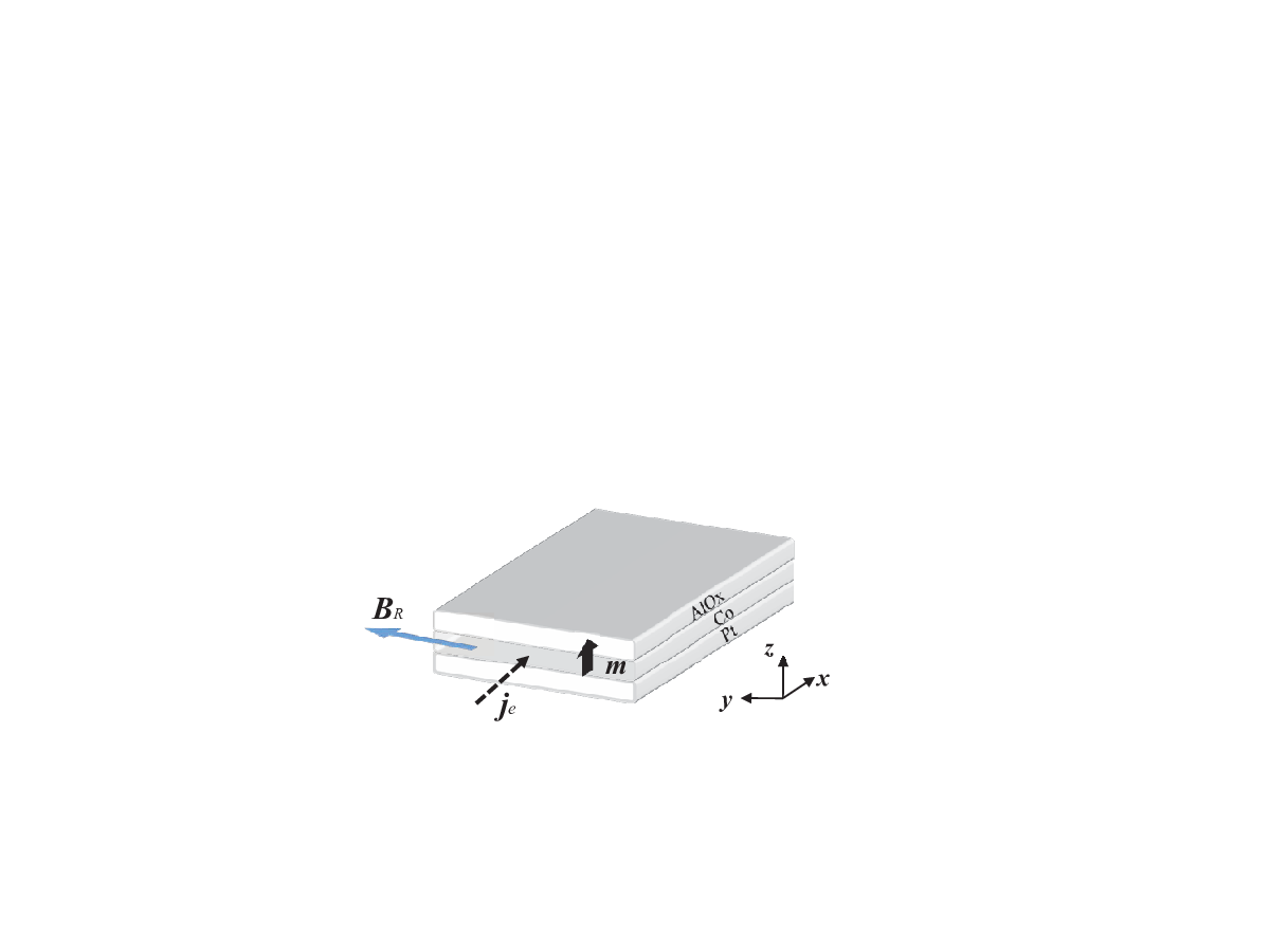
The total Hamiltonian for conducting electrons (with effective mass $m$) in a quasi-two-dimensional ferromagnetic layer in $x-y$ plane is ($\hbar=1$ is assumed throughout)

where $\bm{k}$ is the momentum, $\alpha$ is the Rashba constant, $\hat{\bm{\sigma}}$ the Pauli matrices, $\Delta_{xc}$ the ferromagnetic exchange splitting, $\hat{\bm{m}}$ the magnetization direction, and $H^{i}=\sum_{j=1}^{N}V(\bm{r}-\bm{R}_{j})$ the spin-independent impurity potential with centers located at $\bm{R}_{j}$. An electric field is applied and to be included in the following discourse. Using Dyson equation [25], the advanced and retarded Green’s functions $\hat{G}^{A}$ and $\hat{G}^{R}$, Keldysh function $\hat{G}^{K}$, and the self-energy $\hat{\Sigma}^{A,R,K}$ are related by the quantum kinetic equation [25, 23]

where all Green’s functions are the full functions.

To obtain a diffusion equation from Eq.(2), we assume short-range $\delta$-function type impurity scatterers at low concentration with a weak coupling to electrons [23], then a second-order Born approximation is justified, i.e., $\hat{\Sigma}^{A,R,K}(\bm{r},\bm{r}^{\prime})=\delta(\bm{r},\bm{r}^{\prime})\hat{G}^{A,R,K}(\bm{r},\bm{r})/(m\tau)$. The momentum relaxation rate $1/\tau$ due to spin-independent impurities is evaluated at the Fermi energy. The quasiclassical distribution function $\hat{g}\equiv\hat{g}_{\bm{k},\epsilon}(T,\bm{R})$, as the Wigner transform of the Keldysh function $\hat{G}^{K}(\bm{r},t;\bm{r}^{\prime},t^{\prime})$, is obtained by integrating out the relative spatial-temporal coordinates while retaining the center-of-mass ones $\bm{R}=(\bm{r}+\bm{r}^{\prime})/2$ and $T=(t+t^{\prime})/2$. A gradient expansion on both sides of Eq.(2) followed by a Fourier transform in time domain gives us

where $\hat{\rho}$ is the density matrix. In Eq.(3), $\Omega\equiv\omega+i/\tau$, $b_{k}\equiv|\Delta_{xc}\bm{m}/2+\alpha\bm{k}\times\hat{\bm{z}}|$, the operator $\hat{U}\equiv\hat{\bm{\sigma}}\cdot(\Delta_{xc}\bm{m}/2+\alpha\bm{k}\times\hat{\bm{z}})/b_{k}$, and $\{\cdot,\cdot\}$ denotes the anticommutator.

We solve Eq.(3) according to the discussion outlined in Ref.[23]: find a formal solution $\hat{g}=\mathscr{L}[\hat{K}^{(0)}+\hat{K}^{(1)}]$ in terms of the lowest order approximation

and a higher-order gradient correction

that is accounted by perturbation. We then apply the formal solution in $\hat{K}^{(0)}$ to obtain the zeroth order approximation that is to be substituted into $\hat{K}^{(1)}$ to obtain a gradient correction, thus arriving at the first order approximation to $\hat{g}$. We repeat this procedure to the second order for $\hat{g}$ [23]. This gradient expansion scheme is applicable as long as the spatial gradient of the quasiclassical distribution function is smooth at the scale of Fermi wavelength, i.e. $\partial_{r}\ll k_{F}$.

After angle averaging in momentum space and Fourier transforming the second-order approximation back to real time, we have a diffusion-type equation for the density matrix

where $\hat{\sigma}_{m}\equiv\hat{\bm{\sigma}}\cdot\hat{\bm{m}}$ and we concentrate on quantities at Fermi energy. The diffusion constant is $D=\tau v_{F}^{2}/2$, given $v_{F}$ the Fermi velocity. $\tilde{\Delta}_{xc}=(\Delta_{xc}/2)/(4\xi^{2}+1)$ where $\xi^{2}=(\Delta_{xc}^{2}/4+\alpha^{2}k_{F}^{2})\tau^{2}$. The other parameters in Eq.(6) are

where we identify $\tau_{xc}$ as the D’yakonov-Perel relaxation time. Equation (6) is valid in the dirty limit (i.e. $\xi\ll 1$), which permits the approximation $1+4\xi^{2}\approx 1$ throughout the following discussion. We decompose the density matrix as $\hat{\rho}=n/2+\bm{S}\cdot{\hat{\bm{\sigma}}}$ to introduce the charge density $n$ and the spin density $\bm{S}$. Spin transport in ferromagnetic layers in a real experimental setup [7, 10, 9] is exposed to random magnetic scatterers, for which an isotropic spin-flip relaxation $\bm{S}/\tau_{sf}$ is introduced phenomenologically. In total, we have

where $\bm{\nabla}_{z}\equiv\hat{\bm{z}}\times\bm{\nabla}$. Accounting for both D’yakonov-Perel and random magnetic impurities, rate $1/\tau_{\parallel}\equiv 1/\tau_{xc}+1/\tau_{sf}$ measures the relaxation of the spin density ${\bm{S}}_{\parallel}\equiv S_{x}\hat{\bm{x}}+S_{y}\hat{\bm{y}}$, as $1/\tau_{\perp}\equiv 2/\tau_{xc}+1/\tau_{sf}$ does to $\bm{S}_{\perp}\equiv S_{z}\hat{\bm{z}}$. Parameter $T_{xc}$ sets a time scale for the decay of the transverse (to $\hat{\bm{m}}$) component of the spin density, thus contributing directly to the spin torque [26].

For a broad range of the ratio $\alpha k_{F}/\Delta_{xc}$, Eqs.(7) and (8) govern the full spin dynamics in a ferromagnetic layer and constitute the main result of this Letter. We can readily show [27] that the absence of magnetism ($\Delta_{xc}=0$) leaves the $B$ term a source generating spin density electrically [3, 23]. When spin-orbit coupling vanishes ($\alpha=0$), the first two lines in Eq.(8) survive to describe a diffusive motion of spin density in a ferromagnetic metal, which agrees excellently with early results in the corresponding limit [27, 28]. The $C$ term represents a coherent precession of the spin density around the effective Rashba field. The precession of the spin density (induced by the Rashba field) around the exchange field is described by the $\Gamma$ term, is thus at a higher order (compared to $C$) in the dirty limit for $\Gamma=\Delta_{xc}\tau C/2$. The $R$-term contributes to a magnetization renormalization.

To illustrate the spin dynamics and the Rashba spin torque embedded in Eq.(8), we restore the electric field of strength $\mathscr{E}$ applied along the $\hat{\bm{x}}$ direction by a shift $\bm{\nabla}\rightarrow\bm{\nabla}+e\mathscr{E}\hat{\bm{x}}\partial_{\epsilon}$ [23]. This Letter is focusing on a weak spin-orbit coupling $\alpha k_{F}<\Delta_{xc}$ [11, 12]; i.e., the spin density is aligned dominantly along the local magnetization. Thus, the deviation due to effective Rashba field $\bm{B}_{R}\propto\bm{j}_{e}\times\hat{\bm{z}}$ (along the $\hat{\bm{y}}$ direction in the present setup) is considered as a perturbation. We may approximate the energy derivative $\partial_{\epsilon}\bm{S}\approx P_{F}\mathcal{N}_{F}\hat{\bm{m}}$ and $\partial_{\epsilon}n\approx n_{F}/\epsilon_{F}=\mathcal{N}_{F}$, given $\mathcal{N}_{F}$ the density of states and $P_{F}$ the polarization; both quantities are at Fermi energy $\epsilon_{F}$.

Consider an infinite homogeneous ferromagnetic layer [11], we replace $\bm{\nabla}$ by $e\mathscr{E}\hat{\bm{x}}\partial_{\epsilon}$ and Eq. (8) is

where the higher-order contribution proportional to $R$ is discarded and $\tau_{\Delta}\equiv 1/\Delta_{xc}$ characterizes the time scale of the precession of the spin density around the magnetization. The spin torque exerted on the local magnetization by the nonequilibrium spin density is given by

taking into account a fieldlike spin precession and dephasing of the transverse component that is essentially the Slonczewski-Berger type spin-transfer torque. At a stationary state $\partial\bm{S}/\partial t=0$, Eq.(9) leads to a general form $\bm{T}=T_{\perp}\hat{\bm{y}}\times\hat{\bm{m}}+T_{\parallel}\hat{\bm{m}}\times(\hat{\bm{y}}\times\hat{\bm{m}})$ that is

where $j_{e}=e^{2}n_{F}\tau\mathscr{E}/m$ is the current density, $\zeta=\tau_{\Delta}(1/\tau_{sf}+1/T_{xc})$, $\eta=1+\zeta\tau_{\Delta}/T_{xc}$, and $\beta=\tau_{\Delta}/\tau_{sf}$ [28]. The first term in Eq.(11) is an out-of-plane torque driven by the effective field $\bm{B}_{R}$ and is perpendicular to the ($\hat{\bm{m}}$, $\bm{B}_{R}$) plane. Using the data from experiments [7], we take $\alpha\approx 10^{-10}~\text{eV}\text{m}$, polarization $P_{F}=0.5$, saturation magnetization $M_{s}\approx 1.09\times 10^{6}~\text{A}~\text{m}^{-1}$, and the current density $j_{e}=10^{8}~\text{A}~\text{cm}^{-2}$, the effective field generating the out-of-plane torque is estimated to be of the order of 1 T.

The second in-plane torque arises from the change of the spin density induced by its precession around the exchange field ($\propto\Gamma$) as well as to the presence of spin flip in the layer ($\propto\beta$), inducing a spin density that is parallel to $\bm{B}_{R}\times\hat{\bm{m}}$ (or $\hat{\bm{y}}\times\hat{\bm{m}}$) [27], hence leading to a torque in the ($\hat{\bm{m}},\hat{\bm{y}}$) plane. In other words, the in-plane torque is driven by an effective field along the direction $\bm{B}_{R}\times\hat{\bm{m}}$. In the limit $\tau_{sf}\rightarrow\infty$, the ratio $T_{\parallel}/T_{\perp}\approx\Delta_{xc}\tau/4$, approaches a constant. When considering $T_{xc}\rightarrow\infty$ and $\Gamma\ll C$ (dirty limit), the in-plane torque diminishes and Eq.(11) is in a good agreement with Ref. [11].

The impact of diffusion on the Rashba spin torque is appreciated by numerically solving Eq. (8) in a semi-infinite ferromagnetic wire with a width $L$ along the $y$ axis. The wire is open on the transport direction $\hat{\bm{x}}$, along which an electric field is applied (thus $\nabla_{x}\rightarrow e\mathscr{E}\hat{\bm{x}}\partial_{\epsilon}$). To compare with the recent experiment [9], the magnetization is aligned perpendicularly along ${\hat{\bm{z}}}$. Two boundary conditions are available in the transversal direction ($y$): vanishing spin density ${\bm{S}}(y=\pm L/2)=0$ or vanishing spin current $\mathcal{J}_{y}(y=\pm L/2)=0$ at the boundaries. The former condition indicates an absorbent surface where spin-flip relaxation at the boundaries is fairly strong, thus suppressing the spin density. A vanishing spin current designates a fully reflective boundary where the spin current is reflected. In the present simulation, we choose to adopt the boundary condition according to the work of Kato et al., [29]: optical detection on the spatial profile of the spin density induced by the spin-Hall effect in a $n$-GaAs 2DEG reveals that the spin density vanishes at the interfaces. We believe that the recent experiments on Rashba spin torque in ferromagnetic layers [7, 9, 10] fall into this picture.

Figure 2 shows the spatial profile of the three components of the spin density: $S_{x}$ (panels a and d), $S_{y}$ (panels b and e), and $S_{z}$ (panels c and f), for various magnitudes of $\alpha$.

The spin-orbit interaction drives the spin dynamics in two prominent ways: the first is explained by Edelstein [3]; i.e., a nonequilibrium spin density at $\hat{\bm{y}}$ direction is generated electrically, becoming a source to a nonvanishing $S_{y}$ in the center of the wire. Second, the spin density precesses around the total field combining the exchange ($\Delta_{xc}{\hat{\bm{m}}}\times{\bm{S}}$) and the effective fields ($2C{\bm{\nabla}}_{z}\times{\bm{S}}$). In the case of a wide magnetic wire, this precession is localized near the edges of the wire and vanishes towards the center where the nonequilibrium spin density generated by spin-orbit coupling gets robust along the Rashba field ($\hat{\bm{y}}$ direction). Consequently, the $S_{x}$ component, though much smaller in magnitude than $S_{y}$, is peaked at the boundaries; see Figs.2 (b) and 2(c). The profile of the $S_{z}$ component has an opposite sign at two edges, which is driven by the rotation of the spin accumulation around the effective Rashba fields (pointing oppositely to each other) generated while diffusing transversally along opposite directions (i.e., negative $y$ and positive $y$ axes).

In the case of a weak spin-orbit coupling addressed in this Letter, the spin density profile is mainly symmetric along the (transverse) $y$ direction. In the opposite limit of a strong spin-orbit coupling, the spin-Hall effect induces a large spin imbalance along the transverse direction of the wire, which favors a deeper asymmetry in the spatial profile (not shown here). The narrow width (shorter than the spin-flip diffusion length defined by $\tau_{sf}$) of the wire prevents the relaxation of the spin density such that its effective magnitude in the middle of the wire may differ from its value in an infinite medium.

Therefore, one expects a strong influence of the wire width on the magnitude and sign of the Rashba spin torque. Figures 3(a) and 3(b) display the magnitude of the average torque $\int_{-L/2}^{L/2}\bm{T}dy/L$ at different wire widths as a function of $\alpha$. For a fixed $\alpha$, by decreasing the wire width the in-plane torque $T_{\parallel}$ changes its sign and the magnitude can be enhanced dramatically, while the magnitude of the out-of-plane torque $T_{\bot}$ is just moderately reduced. Figure 3(c) shows the ratio $T_{\parallel}/T_{\bot}$ as a function of the wire width for different spin diffusion lengths. Several features deserve attention. (i) For a given spin-flip relaxation time (therefore the spin diffusion length), the ratio approaches a constant when increasing the width of the wire, while its absolute value increases exponentially when decreasing the width. (ii) For a wide wire with a large spin diffusion length, the ratio tends towards the bulk value $T_{\parallel}/T_{\perp}=\Delta_{xc}\tau/4$. Using the present value $\Delta_{xc}=10^{14}~\text{s}^{-1}$ and $\tau=10^{-15}~\text{s}$, the bulk value is about $0.03$, which agrees well with the numeric value (black solid line) in Fig.3 (c). (iii) The sign of the ratio can be switched by the wire width or the spin relaxation rate, as is reflected in the second term in Eq. (11).

In a recent work, Miron et al., [9] has demonstrated a current-induced magnetization reversal in a perpendicularly magnetized single ferromagnet. In Eq.(11) of this Letter, the effective field (producing the in-plane torque) parallel to $\bm{B}_{R}\times\hat{\bm{m}}$ explains the effective perpendicular magnetic field $\bm{B}_{S_{z}}$ required to accomplish the magnetization switching [9]. In the Co layer as sandwiched by metal oxides and heavy metal with a large spin-orbit coupling, the spin-flip relaxation length is believed to be much shorter than its value in the bulk Co, hence further enhancing the in-plane torque: see Fig.3 (c). If we take $\Delta_{xc}\approx 5\times 10^{14}~\text{s}^{-1}$ (or $0.3~\text{eV}$) [30], $\tau_{sf}\approx 10^{-12}~\text{s}$, and $\tau\approx 10^{-15}~\text{s}$, then we have $\beta\approx 0.002$, $\zeta\approx\tau_{\Delta}/T_{xc}\approx 0.5$, and $\eta$ is of order 1. A quick estimate suggests that the perpendicular switching field generating the in-plane torque is about 100 mT, which agrees with the estimation in Ref.[9]. In the case of magnetic domain walls, the present torque acts like a transverse field that can increase the Walker breakdown limit and enhance the range for the nonadiabatic current-driven domain wall motion [31]. Miron et al., exploited this characteristic to interpret large current-driven domain wall velocities in perpendicularly magnetized domain walls [10].

Most of the previous works on transitions metals have been carried out in fairly complex structures where interfacial Rashba spin-orbit coupling has not been evaluated experimentally or theoretically. Identifying the relevant mechanisms is an urgent need [32]. Among them, the microscopic description of interfacial Rashba spin-orbit coupling in ultrathin layers as well as the spin dynamics in the presence spin-orbit coupling will provide essential information to the electrical manipulation of spins in low dimensional systems.

We are grateful to G. E. W. Bauer, K. -J. Lee, J. Sinova, M. D. Stiles, X. Waintal, and S. Zhang for stimulating discussions.

References

- [1] I. Zutic et al., Rev. Mod. Phys. 76, 323 (2004).
- [2] M. I. D’yakonov and V. I. Perel, Sov. Phys. JETP Lett. 13, 467 (1971).
- [3] V. M. Edelstein, Solid. Stat. Comm. 73, 233 (1990).
- [4] Yu. A. Bychkov and E. I. Rashba, JETP. Lett. 39, 78(1984).
- [5] S. Murakami et al., Science 301, 1348 (2003).
- [6] J. Sinova et al., Phys. Rev. Lett. 92, 126603 (2004).
- [7] I. M. Miron et al., Nature Materials 9, 230 (2010).
- [8] U. H. Pi et al., Appl. Phys. Lett. 97, 162507 (2010).
- [9] I. M. Miron, et al., Nature (London) 476, 189 (2011).
- [10] I. M. Miron et al., Nature Materials 10, 419 (2011).
- [11] A. Manchon and S. Zhang, Phys. Rev. B. 78, 212405 (2008); 79, 094422 (2009).
- [12] A. Matos-Abiague and R. L. Rodriguez-Suarez, Phys. Rev. B 80, 094424 (2009); I. Garate and A. H. MacDonald, Phys. Rev. B 80, 134403 (2009); P. M. Haney, and M. D. Stiles, Phys. Rev. Lett. 105, 126602 (2010).
- [13] K. Obata, and G. Tatara, Phys Rev. B 77, 214429 (2008).
- [14] A. Chernyshov et al., Nature Physics 5, 656 (2009).
- [15] T. Suzuki et al., Appl. Phys. Lett. 98, 142505 (2011); M. Endo et al., Appl. Phys. Lett. 97, 222501 (2010).
- [16] D. Fang et al., Nature Nanotechnology 6, 413 (2011).
- [17] J. C. Slonczewski, J. Magn. Magn. Mater. 159, L1 (1996).
- [18] L. Berger, Phys. Rev. B. 54, 9353 (1996).
- [19] M. D. Stiles and J. Miltat, Top. Appl. Phys. 101, 225 (2006); D. C. Ralph and M. D. Stiles, J. Magn. Magn. Mater. 320, 1190 (2008); J. Z. Sun and D. C. Ralph, J. Magn. Magn. Mater. 320, 1227 (2008).
- [20] M. I. D’yakonov and V. I. Perel, Phys. Lett. 35A, 459 (1971).
- [21] E. G. Mishchenko and B. I. Halperin, Phys. Rev. B 68, 045317 (2003).
- [22] A. A. Burkov et al., Phys. Rev. B 70, 155308 (2004).
- [23] E. G. Mishchenko et al., Phys. Rev. Lett. 93, 226602 (2004).
- [24] I. Adagideli and G. E. W. Bauer, Phys. Rev. Lett. 95, 256602 (2005).
- [25] J. Rammer and H. Smith, Rev. Mod. Phys. 58, 323 (1986).
- [26] A. Brataas et al., Phys. Rev. Lett. 84, 2481 (2000); M. D. Stiles and A. Zangwill, Phys. Rev. B 66, 014407 (2002); Y. Tserkovnyak et al., Rev. Mod. Phys. 77, 1375 (2005).
- [27] X. Wang and A. Manchon, arXiv:1111.5466.
- [28] S. Zhang and Z. Li, Phys. Rev. Lett. 93, 127204 (2004).
- [29] Y. K. Kato et al., Science 306, 1910 (2004).
- [30] The exchange splitting in the bulk of Co is typically of order 1 eV and we expect a lower value in the ultrathin film.
- [31] M. T. Bryan et al., J. Appl. Phys. 103, 073906 (2008); S. Glathe et al., Appl. Phys. Lett. 93, 1162505 (2008).
- [32] See, for example, L. Liu et al., Phys. Rev. Lett. 106, 036601 (2011).