Achievable and Crystallized Rate Regions of the Interference Channel with Interference as NoiseThanks: Manuscript received March 20, 2011; revised September 10, 2011. This work is partially supported by NSF CNS-0953377, CNS-0905556, CNS-0910461, and ECCS-1028782. The material in this paper was presented in part at Allerton Conference on Communication, Control, and Computing, Allerton, USA, September 2007 [1], and at the IEEE International Conference on Communications, Dresden, Germany, June 2009 [2]. M. Charafeddine was with the Department of Electrical Engineering at Stanford University, CA, USA, and he now works at ASSIA, Redwood City, CA, USA (e-mail: mohamad@stanfordalumni.org). A. Sezgin is with the Department of Electrical Engineering and Information Technology at Ruhr-University Bochum, Germany (e-mail: aydin.sezgin@rub.de). Z. Han is with the Electrical and Computer Engineering Department, University of Houston, Houston, TX, USA, and with the Department of Electronics and Radio Engineering, Kyung Hee University, Yongin, Gyeonggi, South Korea (e-mail: zhan2@mail.uh.edu). A. Paulraj is with the Department of Electrical Engineering at Stanford University, CA, USA (e-mail: apaulraj@stanford.edu). Copyright ©2011 IEEE. Personal use of this material is permitted. However, permission to use this material for any other purposes must be obtained from the IEEE by sending a request to pubs-permissions@ieee.org.
Abstract
The interference channel achievable rate region is presented when the interference is treated as noise. The formulation starts with the user channel, and then extends the results to the user case. The rate region is found to be the convex hull of the union of power control rate regions, where each power control rate region is upperbounded by a -dimensional hyper-surface characterized by having one of the transmitters transmitting at full power. The convex hull operation lends itself to a time-sharing operation depending on the convexity behavior of those hyper-surfaces. In order to know when to use time-sharing rather than power control, the paper studies the hyper-surfaces convexity behavior in details for the user channel with specific results pertaining to the symmetric channel. It is observed that most of the achievable rate region can be covered by using simple On/Off binary power control in conjunction with time-sharing. The binary power control creates several corner points in the dimensional space. The crystallized rate region, named after its resulting crystal shape, is hence presented as the time-sharing convex hull imposed onto those corner points; thereby offering a viable new perspective of looking at the achievable rate region of the interference channel.
I Introduction
One important communication model in wireless communication is the interference channel, which is subject to intensive research nowadays. For example, the model is relevant for cellular networks in which multiple base stations transmit data to their respective subscribers and thereby causing interference at the unintended receivers, and ad-hoc networks in which nodes are active at the same moment in the same frequency band. For a better understanding of the interference channel, it is crucial to know its capacity region, i.e., the maximum set of all achievable rate points. It serves also as a benchmark for the comparison of different schemes. Unfortunately, the capacity region of the user interference channel has been an open problem for about years [3, 4]. Information-theoretic bounds through achievable rate regions have been proposed, most famously with the Han-Kobayashi region [5]. The capacity of the Gaussian interference channel under strong interference has been found in [6, 7]. Recent results on the user interference channel to within one bit of capacity have been shown in [8], where a simplified Han-Kobayashi scheme was used in which the message is split in two parts, the private part and the common part. The transmit signal is then a superposition of those two signals. By a smart allocation of power between those two parts it was shown that this scheme is asymptotically optimal using a new metric, which is referred to as the generalized degrees of freedom. The generalization of the obtained results to the -user case is rather difficult. As such, for the -user case mainly the capacity slope as a function of the Signal-to-Noise-Ratio (SNR) are known. It was shown in [9] that for very high SNR, the capacity can be approximated by , where the second term vanishes by definition for extremely high SNR.
The aforementioned referenced literature focused mainly on the user interference channel from an information-theoretic point of view with highly sophisticated and thus quite complicated transmitters and receivers. There are other works in literature that tackle the practical issues in order to improve the performance of the interference channels. Power control is one element of critical importance. In [10], a framework for the uplink power control is constructed and iterative power control is proposed. Adaptive modulation and coding (AMC) can be combined with power control to enhance the network performance [11]. For multiple channel (such as OFDM) and multiple cell case, joint AMC and power control have been widely employed [12]. Beamforming and spatial diversity can also be utilized when communicating over the MIMO channel [13]. Interference avoidance [14] has also attracted many recent attentions. Finally, many distributed solutions are proposed [15, 16, 17] with the benefit of simple implementation or low data overhead.
In this paper, the achievable rate region is discussed for the user interference channel when the interference is treated as additive Gaussian white noise and no multi-user detection is employed. Examples where we encounter the need to define such rate region are found in multicell communications, in addition to mesh and sensor networks where the preference is to use low-complexity transceivers. It is also interesting to note that using the strategy of treating interference as additional noise proves to be asymptotically optimal, i.e., it was shown in [8] that treating interference as noise is optimal, as long as the interference power in dB is lower than half of the useful signal power given that the power to noise ratio is asymptotically high. This result was extended to the non-asymptotic case independently by three research groups [18, 19, 20]. The generalization to the asymmetric case and the user interference channel is given in [18, 19, 20] as well, where it was shown that it is optimal to treat the interference as noise whenever a similar (sufficient) condition holds. The references [18, 19, 20] considered only the Gaussian interference channel, while the general discrete many-to-one and one-to-many memoryless channels were investigated in [21]. It was shown in [21] that treating interference as noise is also optimal in the discrete memoryless channel as long as the received signal at the interfered receiver is stochastically degraded compared to the received signals of the other receivers. The optimality of treating interference as noise for the multiple antenna case has been considered by [22, 23, 24].
This paper finds the achievable rate region for the user interference channel as the convex hull of the union of rate regions formed via power control, where each rate region is upperbounded by a hyper-surface of dimension characterized by having one of the transmitters operating at full power. Given that there is a convex hull operation imposed onto the hyper-surfaces, it is important to know their convexity behavior in order to determine when time-sharing should be applied. This is treated in details for the user interference channel. As the convex hull operation lends itself naturally to a time-sharing operation, and based on the convexity conditions found, the paper discusses when a time-sharing strategy should be employed rather than pure power control, and then presents specific results pertaining to the user symmetric channel. It is observed that the achievable rate region can be practically approximated by using simple On/Off binary power control in conjunction with time-sharing. The On/Off binary power control creates several corner points in the dimensional rate region, and employing a convex hull time-sharing operation on those points achieves what is denoted as a crystallized rate region.
The system setup is presented in section II. Section III discusses the achievable rate region for the user interference channel, and then generalizes the results to the user case. Section IV focuses on characterizing the user rate region in terms of convexity or concavity and when time-sharing is optimal with specific results to the symmetric channel. Section V introduces the concept of the crystallized rate region where time-sharing and On/Off binary power control are used. Finally, the conclusion is drawn in section VI.

II System Model
The user interference channel is presented in Fig.1 with transmitters and receivers. The transmitter transmits its signal to the intended receiver with power . The receivers have independent additive complex white Gaussian noise with zero mean and variance of . Each transmitter is assumed to have a peak power constraint of . Each transmitter has a single antenna and communicates over a frequency flat channel. denotes the channel power gain received at the receiver from the transmitter. Therefore, is the channel gain of the desired signal, whereas with represents the interfering channel gain. P is the transmit power vector of length , where the element denotes the transmit power of the transmitter. The interference is treated as additive noise throughout this paper. denotes the maximum reliable rate of communication for the transmit-receive pair. Therefore, the achievable rate for the transmit-receive pair is written as:
| (1) |
The next section finds the achievable rate region for such transmit-receive pairs.
III Achievable Rate Region Frontiers for the Interference Channel
First, the section considers the user interference channel. The rate region problem is analyzed by formulating its underlying nonconvex power control problem, for which we find a closed form analytical solution. The rate region is described by finding the maximum possible data rates achievable when each user is subject to a maximum transmit power constraint. This section then introduces the user case to study the effect of adding a new dimension; and finally, by induction, the result is generalized for the user case.
III-A -user Achievable Rate Region Frontiers
In the case of the user interference channel, Eq. (1) can be expressed as a function of and as . For notational brevity, the channel gains are normalized by the noise variance, specifically: , , , and . and can therefore be written as:
For notational brevity, denotes a point in the rate region marked by having and . Effectively, the coordinate of is , and the coordinate of is . The first objective is to find the achievable rate region frontiers of Eq. (III-A) through power control of and , where each transmitter is subject to the maximum power constraint of . The frontier herein denotes the line (or generally, the -dimensional surface for the user channel) which traces the rate region via power control.
III-B Rate Region Frontiers Formulation
The rate region frontier can be traced by setting to a certain value , and then by sweeping over its full possible range from to while finding the maximum value that can be achieved for each . From Eq. (III-A), is monotonically increasing in and monotonically decreasing in , thus point corresponds to point on the axis in Fig. 2, representing the maximum value can attain. Similarly for the axis, the maximum value that can attain is , alternatively corresponding to point . Those points represent the cases in which one of the users is silent, while the other is transmitting at full power. Similarly, point has the coordinates of and .

Hence, for a constant rate ,
| (4) |
Therefore, the relation between and is obtained as follows:
| (5) |
From Eq. (5), for a constant , can now be written as a function of one parameter as , for , specifically:
| (6) |
It is important to analyze the behavior of in terms of . This is presented in the following lemma:
Lemma 1.
Setting at a constant rate, , is a monotonically increasing function in .
Proof:
The proof is provided in Appendix A. ∎Using this lemma, the following corollary of uniqueness property is obtained:
Corollary 1.
For every rate tuple , there is a unique power tuple .
Proof:
i) a direct implication of monotonicity in Eq. (6) is that if is equal to a constant at the rate of , then there is a unique that achieves , ii) when is determined, then is uniquely defined from Eq. (5), iii) from and , is uniquely defined as from Eq. (4). Thus, and uniquely define a point in the rate region with coordinates and . ∎In other words, any point in the rate region is achieved solely by a unique power tuple. This leads to what we denote by potential lines in the rate region, which are formed by holding one power dimension constant to a certain value and sweeping the other power dimension over its full range. In that regard, to describe a potential line marked by having held at a constant power , we use the following notation to be equivalent to where and . Based on the uniqueness property just discussed, we have the following corollary (illustrated in Fig.3):
Corollary 2.
Potential lines11 1 The property in Corollary 2 is the reason for denoting these lines as potential lines, where the nomenclature is borrowed from electromagnetics based on a similar property for equipotential lines of an electric field [25]. along one power dimension do not intersect, i.e., and do not intersect if .


The problem of finding the power control rate region frontiers then simplifies into finding the maximum value that can be achieved for any value of . Effectively, the formulation of the power control rate region is:
is swept over the full range of , i.e., . The power control optimization problem in Eq. (III-B) is not straightforward as it is a nonconvex problem [26]. However, by splitting the rate range of into two intervals: Interval 1 for and Interval 2 for , we are able to find a closed form analytical solution for each interval. The analysis of the optimization problem in Eq. (III-B) over these two intervals follows in the next two subsections.
III-C Frontier for Interval 1:
As Eq. (4) is monotonically increasing in and monotonically decreasing in , can only exceed when is less than . Thus, is attainable only when , and needs to be less than otherwise. From the proof provided for Lemma 1, where Eq. (6) is proved to be monotonically increasing in , and for the following Interval 1 range of : , the solution to the optimization problem is:
| (10) |
Therefore, in this range of , using Eq. (5) and Eq. (10), is expressed by a function of as follows:
| (11) |
Over this Interval 1 range of , the relation found in Eq. (11) describes the expression governing the potential line , in which is held at constant maximum power and sweeps its full range from to . For brevity, the potential line is denoted as , where the second power dimension, , is held at the maximum power. In this range of , defined by Eq. (11) represents a power control frontier of the rate region as shown in Fig.2.
III-D Frontier for Interval 2:
Using symmetry of the previous result, for a constant rate , there is a linear relation between and . Thus, can be written in function of one parameter as follows:
| (12) |
By symmetry of the result in Lemma 1, is monotonically increasing in . Thus, by symmetry, for the following range of : we have:
| (13) |
Basically, the value found in Eq.(13) describes the frontier for the following rate ranges of: and – similar to the former subsection III-C where described the frontier for the following rate ranges of: and .
Therefore, the value of at the frontier is:
| (14) |
Hence, for this Interval 2 range of : , the value of that achieves the frontier follows as:
| (15) |
So effectively, the value found in Eq. (15) is the answer for the optimization problem in Eq. (III-B) for this range of . Explicitly, for , we have:
| (16) |
Therefore, in this range of , using Eq. (15) and Eq. (6), is expressed in function of as follows:
| (17) |
The relation found in Eq. (17) describes the expression governing the potential line , where is held at a constant maximum power and sweeps its full range from to . Similarly for brevity, the potential line is denoted as . In this range of , as defined by Eq. (17) represents a power control frontier of the rate region as shown in Fig.2.

III-E The User Achievable Rate Region
This subsection consolidates the two earlier results to fully describe the rate region frontiers.
In Fig.4, point A denotes point (user transmitting solely at full power), point B denotes point (both users are transmitting simultaneously at full power), and point C denotes point (user transmitting solely at full power).
The rate region for a user interference channel achieved through power control is obtained as:
| (20) |
Finally, the user rate region, denoted as , is found as the convex hull of the power control rate region. It is defined as:
| (21) |
The treatment of the achievable rate region for the user interference channel follows next. It starts by considering a user interference channel to show the effect of adding a new dimension, and then generalizes the result for the user case.
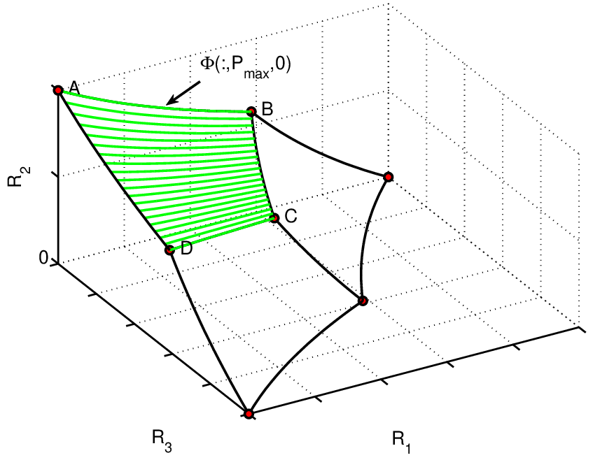
III-F User Example: Effect of Increasing from to
The rate region for the user case is illustrated in Fig.5. The following notation of denotes a point in the rate region with coordinates of , , . Accordingly, describes a line characterized by sweeping the transmit power of the first transmitter from to , with the second transmitter transmitting at and the third transmitter transmitting at a power value of . Similarly, represents a surface in the rate region marked by sweeping the full range of and , and holding at .
When , the same setup and results that are described earlier in this section applies. Thus, for the rate range of and and , the frontier can be described as , which is the potential line from point A to point B in Fig. 5. As increases, the goal is to describe its effect and how it is traced in the rate region.
Revisiting Eq. (1), a fixed has the effect of just an additive noise term in and . Hence, all the previous results in section III are applicable for any value of in describing the frontier for and , since the effect of can be lumped in the noise term. Thus, for the range of and , where is constant, the frontier line on and is , i.e., characterized by having . Consequently, the potential lines (or surfaces) concept in the user case carries through.
Next, the frontier on is described. For each value of , traces one of the highlighted curves in Fig. 5. For the collection of lines to form a frontier, we want to prove that at each increasing value of these non-intersecting potential lines monotonically increase in the dimension. This is evident from the relation between and in Eq. (1). The maximum value of that can be achieved in this case is when , i.e., . Therefore, the highlighted frontier surface in Fig. 5 is the closed potential surface . The boundary contours of this surface are the potential lines: , , , and , defined as , , , and , respectively.
By symmetry of interchanging , , and , the user rate region is found via the convex hull onto the union of the regions bounded by these three surfaces: , , and . The rate region is therefore expressed as: where is the region outer-bounded by the potential surface , where is the surface characterized by having in the power position. (Note that the intersection of potential surfaces is a potential line, as two of the dimensional inputs become equal, i.e., and .)
III-G User Generalization
The case for user generalization is done by induction. For the added dimension to the existing dimensions problem, the additional power effect of can be lumped in the additive noise term of the existing expressions, and thus the results for hold and carry through. The potential hyper-surfaces for fixed are non-intersecting and monotonically increasing in , and thus the maximum outer limit is reached with for the appropriate range of . Invoking symmetry, we can generalize over all the rates ranges, therefore arriving to the following theorem.
Theorem 1.
The achievable rate region of the user interference channel by treating the interference as noise is:
| (22) |
, where is a hyper-surface frontier of dimensions, characterized by holding the transmitter at full power.
Note that Theorem 1 also holds for different thermal noise levels or different maximum power levels.
IV Convexity Characteristics of the Power Control Frontiers For the User Interference Channel
This section focuses on the user interference channel and studies the behavior of the power control frontiers, i.e., the potential lines and , in terms of convexity and concavity in order to determine when the convex hull operation entails employing time-sharing. This happens whenever any of the potential lines, or segment thereof, is convex, which enables higher data rate to be achieved using time-sharing rather than using power control. Furthermore, specific results pertaining to the symmetric channel are presented at the end of this section.
The power control frontiers equations for the user case are:
- •
: ,
- •
:
It is not clear when is convex or concave, or whether it can exhibit a non-stationary inflection point. The non-stationary inflection point happens when the potential line has simultaneously a convex segment and a concave segment. The convexity behavior is thus treated next in more details.
IV-A Convexity or Concavity of the Power Control Frontiers
By using Eq. (5) when , the potential line depends on through the following relation of and :
Therefore, the second derivative of with respect to leads to the following expression in function of :
| (23) |
where .
If the potential line is concave (i.e. ) then the enclosed region is convex. The rate region is defined to be convex when a straight line connecting any two points inside the rate region is entirely enclosed in the rate region. In contrast, if the potential line is not concave, i.e., if it is convex or exhibits a non-stationary inflection point, then we describe its enclosed region as being concave; as in this situation, the aforementioned definition of a convex region does not hold. In summary, if is concave, then is convex, and is concave otherwise.
Let be the real operation, the inflection threshold is defined as:
| (24) |
where was derived such that Therefore, it suffices to study convexity or concavity of potential line by examining the sign of . Note that the inflection threshold only depends on system parameters , , , , and . The relation is nonlinear. By plugging in the respective values, the convexity behavior is assessed, and it can be decided whether time-sharing is needed.
Thus, can exhibit the following convexity behaviors:
- •
: then for all the range of , thus is concave. Operating via power control is optimal in leading the highest achievable data rate, and no time-sharing is needed. See in case (i) in Fig.6.
- •
- •
: then for all the range of , thus is convex. See in cases (iii) and (iv) in Fig.6. Depending on the , , , , and parameters, it is optimal to apply time-sharing with the following options:
- –
between point A and point B, see Fig.7 (c).
- –
between point A and a point on the concave segment of , see Fig.7 (b).
- –
between point A and point C, see Fig.7 (d). This is effectively Time Division Multiplexing (TDM), where each user transmits solely at any point of time. This form of dimension-orthogonality occurs when the interference is very strong rendering the cost too high for having simultaneous transmission. The upcoming subsection IV-B explores the optimality of operating via TDM, or equivalently, it explores when this cost is deemed too high.
- –


By symmetry, the potential line exhibits similar convexity behavior: a) it is convex when , b) it is concave when , and c) it exhibits a non-stationary inflection point when . Hereby, with , the inflection threshold is defined as:
| (25) |
Note that by virtue of how the inflection threshold is situated with respect to power , whenever any of the potential lines exhibit an inflection point, the order of which segment is convex or concave is not arbitrary. It always starts concave in the segment closer to the coordinate axis. Explicitly, if and exhibit inflection points, then tracing the rate region from left to right: is concave then transitions to convexity, and is convex then transitions to concavity.
IV-B When is TDM Optimal?
Discounting the case when or exhibit non-stationary inflection point for simplicity, and focusing on the case when both potential lines are convex (i.e., and ), it is important to know when TDM is optimal. Under the aforementioned assumption, this translates to determine when time-sharing between point A and point C is better than time-sharing through intermediate point B. This is done by comparing the y-axis ordinate of point B, , relative to the y-axis ordinate from the straight line connecting points A and C at , denoted as , as shown in Fig.7 (d). Namely, TDM is optimal when ; that is:
This leads to the following Lemma 2.
Lemma 2.
Operating via TDM (i.e. one transmitter solely transmitting at a certain time) is optimal in achieving the rate region when
| (28) |
with .
IV-C Symmetric User Interference Channel
This subsection treats the symmetric user channel, mainly analyzing the expression in Eq. (28) in order to derive clear insights. For the symmetric channel, and , the expression in Eq. (28) simplifies, and leads to the following corollary on the TDM optimality condition:
Corollary 3.
For the symmetric user interference channel, operating via TDM is optimal in achieving the rate region when
| (29) |

In other words, when the interference is weak (i.e., is below the threshold
in Eq. (29)), then it is best for both transmitters to transmit
at full power. When the interference increases and
exceeds the threshold in Eq. (29), then the TDM
scheme becomes optimal. In this scenario, the users can no longer share the same
resource, and thus they have to use it in an orthogonal fashion. An example is
illustrated in Fig.8. The application of the usage of the different
types of time-sharing and the advantage over power control has been
discussed in [27], when it was applied to a
sector interference channel in a cellular setting.
Remark: For high SNR (i.e. ), Eq. (29)
reduces to , which coincides with the results
in [8]; where this condition marks
the interference power threshold above which treating the interference as noise
is no longer optimal in the Degrees of Freedom sense and no longer within a gap
of -bit from achieving capacity.
In addition, Appendix B proves that the expression in Eq. (29) is a sufficient condition for both frontiers and to be convex, i.e., and are always ; which is the starting necessary condition of subsection IV-B when treating the general asymmetric channel. Therefore, when satisfies the expression in Eq. (29), the frontiers potential lines are always convex and TDM is optimal.
The extension of Corollary 3 to the user symmetric interference channel is provided in Appendix C, leading to the following TDM optimality condition when:
| (30) |


V Crystallized Rate Region
Based on the discussion in the previous two sections, this section introduces a novel approach into simplifying the rate region in the dimensional space by having only an On/Off binary power control. This consequently leads to corner points within the rate region. By forming a convex hull through time-sharing between those corner points, it thereby leads to what we denote a crystallized rate region [2]. The concept of the crystallized rate region has since been extended to the MIMO and the MIMO-OFDM channels [28, 29]. This section focuses on the crystallized rate region formulation and its evaluation.
As illustrated in Fig.9 for the user case, the crystallized rate region is an approximation of the achievable rate region formed by a convex hull of straight lines connecting points A, B, and C. Those corner points are achieved through binary power control with the transmitters employing either zero or full power. For the user interference channel, there exist corner points; similarly for the user case, there exist corner points. Note that in Fig.9, the time-sharing convex hull connects point A and point C though point B; whereas if the interference is strong, the convex hull is formed by time-sharing A and C only. Fig.10 shows an example of the user case where Fig.10 (a) is the crystallized hull, and Fig.10 (b) is the crystallized hull overlaid on top of the power control rate region.


In the user dimension, the time-sharing convex hull is a set of straight lines connecting two points. In the user dimension, it is a set of polygon surfaces connecting three points, see Fig. 11. In the user dimension, each polygon is formed by connecting points, and hence the number of such polygons is .
V-A System Time-sharing Coefficients and New Rates Equations
Recall that with power control, the achievable rates for the user interference channel are given in Eq. (III-A). The paradigm with the crystallized rate region approach is different. Instead of formulating the problem as a power control problem for finding , the crystallized rate region formulation focuses on finding the appropriate time-sharing coefficients of the corner points. For the user case, let , , denote the system time-sharing coefficients vector of respective corner points (user 1 transmitting solely with a time-sharing coefficient ), (user 2 transmitting solely with a time-sharing coefficient ), and (both users transmitting with a time-sharing coefficient ). The reason for labeling a system time-sharing coefficients vector is to emphasize the combinatorial element in constructing the corner points, where the cardinality of .
For user case, in contrast with Eq. (III-A), the rates and for the crystallized region are:

Any solution point on the crystallized hull lies somewhere on a time-sharing line connecting two points for the user case; and similarly in the user case, the solution point lies somewhere on a time-sharing plane connecting three points (see Fig.11), then by induction we obtain the following corollary:
Corollary 4.
For any solution point on the user crystallized rate region, the system time-sharing vector has at maximum nonzero coefficients out of its elements.
Corollary 4 could also have been reached invoking the Carathodory theorem [30], where, in the paper’s context, any point lying on the hyper-surface of dimension is enclosed in a convex set of or fewer points inside the hyper-surface. Therefore, if those points are the corner points, any solution point on the -dimensional hyper-surface will be the result of time-sharing at maximum corner points.
Let (k) denote the transmitters power mask that characterizes the corner point, specifically:
is the action taken by the user in characterizing the corner point; the binary transmit action is either being silent or transmitting at full power. Let indicate the interferers transmit power mask, which is derived from vector (k) by excluding the transmitter’s action. The generalization for the user crystallized rates equations now follows as:
| (36) |
where is the desired channel gain from the transmitter to the receiver normalized by the noise power; i is the noise-normalized channel gains vector received at the receiver from all the transmitters excluding the transmitter. The length of each vector and i is .
V-B Evaluation of Crystallization
In this section, we compare the crystallized rate region and the rate region bounded by the power control potential lines. In effect, we are evaluating how much gain or loss results from completely replacing the traditional power control scheme (see Eq. (III-A)) with the time-sharing scheme between the corner points (see Eq. (V-A)). For this purpose, we consider the symmetric channel, where , and we increase the interference to vary the signal to interference ratio . Two metrics are used as a measure: (a) the area of the rate region, and (b) the maximum bit rate gap between the traditional power control and the crystallized rate region scheme.
The values of the area bounded by the power control potential lines and the area bounded by the crystallized rate region are plotted in Fig.12(a). For weak interference, or equivalently noise-limited regime, point B is used in constructing the crystallized region. As the interference increases beyond a certain threshold level, time-sharing through point B becomes suboptimal, and time-sharing A-C becomes optimal. The exact switching point between power control to time-sharing is given in Eq.(29). In Fig.12(a), this happens at the intersection of the time-sharing line through point B and the A-C time-sharing line. As indicated in Fig.12(a), there is no significant loss in the rate region area if time-sharing is used universally instead of traditional power control; in fact in some cases time-sharing offers considerable gain. Specifically, whenever the potential lines exhibit concavity, time-sharing loses to power control; whenever the potential lines exhibit convexity, time-sharing wins over power control. Different values of also lead to the same conclusion.


The second measure, the maximum rate gap percentage between the rate achieved by traditional power control and the rate achieved by using the crystallized rate region is plotted in Fig.12(b). The maximum bit rate loss of using the crystallized hull compared to power control does not exceed , and the crystallized strategy is therefore quite attractive. It is arguable that as the interference becomes the network bottleneck there is little reason to implement non-binary power control, and that dimension orthogonalization becomes the primary objective.
VI Conclusion
The achievable rate region for the user interference channel was presented when the interference is treated as noise. The results were first found for the user interference channel, then they were extended to the user case to show the effect of adding an additional dimension. Subsequently, they were generalized for the user case. The user rate region was found to be the convex hull of the union of the rate regions, where each rate region is upperbounded by a -dimensional hyper-surface characterized by having one of the transmitters transmitting at full power. For the user interference channel, those hyper-surfaces become what the paper refers to as power control potential lines. Hence, to determine when time-sharing should be used in forming the achievable user rate region, the paper studied the potential lines convexity behavior. Finally, the novel concept of the crystallized rate region was introduced and evaluated. The crystallized rate region is described by composing a time-sharing convex hull onto the corner points obtained from On/Off binary power control. The evaluation of the crystallized rate region shows little value in the implementation of non-binary power control compared to the use of binary power control in conjunction with time-sharing. In effect, the crystallized rate region approach offers a new perspective of looking at the achievable rate region of the interference channel.
Appendix A Proof that is Monotonically Increasing in
Proof:
Effectively, Eq. (6) is in the form of . As is monotonically increasing in its argument, it suffices to prove that is monotonically increasing in . Therefore, define as:
| (37) |
| (38) |
The numerator in Eq. (38) is nonzero if and ( or are the trivial cases where the rate region is either a line or the point zero). As , then . Thus is always for non-trivial cases of and . Thus, is monotonically increasing in , and equivalently is monotonically increasing in . ∎
Appendix B Proof that Eq. (29) is a Sufficient Condition for Both and to be Convex
Proof:
For the symmetric case, can be written as
where . can also be written in this form:
where , and . From the expression in Eq. (29), can be alternatively upper-bounded as . Therefore, is upper-bounded as:
| (39) |
From Eq. (39), is always negative. however can be positive or negative, evaluated as follows:
- •
: then , and as is always positive, then .
- •
: is . In this case, the numerator of can be written as:
Given the fact that , then can be upper-bounded as:
Hence, the frontiers potential lines and are convex. ∎
Appendix C Extension of Corollary 3 to the user case
Focusing on the 2D rate region of an user symmetrical rate region, if Eq. (29) is satisfied, Appendix B proved that it is a sufficient condition to make sure that and are convex and that they do not have an inflection point. Let denote the threshold value in Eq. (29). Hence, if the interference channel gain , then and in the 2D rate region are convex. As more users transmit, they will cause additional interference power on and . Taking the user case as an example, if the user transmits, then . Projecting the 3D rate region into the 2D plane will lead to , where , which is greater than . Thus, if the 2D rate region have a convex and , then ; and projecting higher dimensional rate region frontiers into the 2D plane will always result in power control frontiers, denoted as and , that are always convex – due to the fact that they can be obtained using an interference power gain where .
The goal of this appendix section is to find the user symmetrical interference channel gain threshold, denoted as , such that when , TDM is optimal in leading higher achievable rate region. Thus, as a starting assumption (which is proved to hold later on), assume ; which therefore leads to the property that all the dimensional hypersurfaces are convex – as the projections on all the pair-wise 2D planes result in convex power control frontiers.
With a TDM solution, users transmissions are orthogonal in time, and therefore, whenever user transmits all other users are silent. The maximum TDM rate achievable for user is when , and in the context of an user symmetrical channel, it is equal to , and . Therefore, whenever user transmits under TDM, its maximum achievable rate in the dimensional rate region is a point on the axis with a value equals to ; let denotes such a point.
Let be a hyperplane formed by connecting via time-sharing the points. Define the origin point O as the point with coordinates . Define point B on the power control achievable rate region when all users transmits at the same time; thus point B coordinates are . Define point B’ on the time-sharing hyperplane when all users transmits in TDM for an equal amount of time. Let denotes a vector from point O to point B, and similarly, denotes a vector from point O to point B’. Let denotes the vector length; for instance, for , is the distance from point O to point B. Therefore, a time-sharing TDM solution is optimal when ; which has the interpretation of the hyperplane leading higher achievable rate region than the power control hyper-surfaces frontiers.
Based on the aforementioned coordinates of point B, . For , it is the shortest distance from point O to the hyperplane ; which is equal to the absolute value of the dot product of the unit normal vector of and the vector , where point K is a point on . The unit normal vector of is equal to . By choosing point K to be equal to the point on the axis, , where has been defined earlier to be equal to . Therefore, .
Hence, a time-sharing TDM solution is optimal when
| (41) |
Expanding Eq. (41) leads to Eq. (30). The threshold is monotonically increasing for a positive , which starts at Eq. (29) for and flattens out asymptotically for large n. Using the first order approximation of to , asymptotically converge to:
independent of the number of users .
References
- [1] M. Charafeddine, A. Sezgin, and A. Paulraj, “Rate region frontiers for user interference channel with interference as noise,” Proc. Allerton Conference on Communication, Control, and Computing, Allerton, IL, September 2007.
- [2] M. Charafeddine, Z. Han, A. Paulraj, and J. Cioffi, “Crystallized rates region of the interference channel via correlated equilibrium with interference as noise,” Proc. IEEE International Conference on Communications (ICC), Dresden, Germany, June 2009.
- [3] H. Sato, “Two-user communication channels,” IEEE Trans. on Information Theory, vol. 23, no. 3, pp. 295–304, May 1977.
- [4] ——, “On degraded Gaussian two-user channels,” IEEE Trans. on Information Theory, vol. 24, no. 5, pp. 637–640, September 1978.
- [5] T. Han and K. Kobayashi, “A new achievable rate region for the interference channel,” IEEE Trans. on Information Theory, vol. 27, no. 1, pp. 49–60, January 1981.
- [6] H. Sato, “The capacity of the Gaussian interference channel under strong interference,” IEEE Trans. on Information Theory, vol. 27, no. 6, pp. 786–788, November 1981.
- [7] A. B. Carleial, “Interference channels,” IEEE Transactions on Information Theory, vol. 24, no. 1, pp. 60-70, Jan. 1978.
- [8] R. Etkin, D. Tse, and H. Wang, “Gaussian interference channel capacity to within one bit,” IEEE Transactions on Information Theory, vol. 54, no. 12, December 2008.
- [9] V. Cadambe and S. Jafar, “Interference alignment and degrees of freedom of the user interference channel,” IEEE Transactions on Information Theory, vol. 54, no.8, August 2008.
- [10] R. Yates, “A framework for uplink power control in cellular radio systems,” IEEE J. Select. Areas Commun., vol. 13, no. 7, pp. 1341–1348, September 1995.
- [11] E. Armanious, D. D. Falconer, and H. Yanikomeroglu, “Adaptive modulation, adaptive coding, and power control for fixed cellular broadband wireless systems: Some new insights,” in Proc. IEEE Wireless Communications and Networking Conf. (WCNC03), 2003.
- [12] H. J. Su and E. Geraniotis, “A distributed power allocation algorithm with adaptive modulation for multi-cell ofdm sytems,” in 5th IEEE International Symposium on Spread Spectrum Techniques and Applications, 1998.
- [13] Z. Han and K. J. R. Liu, “Power minimization under throughput management over wireless networks with antenna diversity,” IEEE Transactions on Wireless Communications, vol. 3, no. 6, pp. 2170–2181, November 2004.
- [14] D. C. Popescu and C. Rose, Interference Avoidance for Wireless Systems. John Wiley and Sons, Inc, 2003.
- [15] C. Saraydar, N. Mandayam, and D. Goodman, “Efficient power control via pricing in wireless data networks,” IEEE Transactions on Communications, vol. 50, no. 2, pp. 291–303, Feburary 2002.
- [16] J. E. Hicks, A. B. MacKenzie, J. A. Neel, and J. H. Reed, “A game theory perspective on interference avoidance,” in IEEE Global Telecommunications Conference, 2004.
- [17] Z. Han, D. Niyato, W. Saad, T. Basar, and A. Hjorungnes, Game Theory in Wireless and Communication Networks: Theory, Models and Application. Cambridge University Press, 2011.
- [18] A. S. Motahari and A. K. Khandani, “Capacity bounds for the Gaussian interference channel,” IEEE Transactions on Information Theory, vol. 55, no. 2, pp. 620–643, February 2009.
- [19] V. S. Annapureddy and V. V. Veeravalli, “Sum capacity of the Gaussian interference channel in the low interference regime,” Proc. ITA Workshop, San Diego, CA, Jan-Feb, 2008.
- [20] X. Shang, G. Kramer, and B. Chen, “A new outer bound and the noisy-interference sum-rate capacity for Gaussian interference channels,” IEEE Transactions on Information Theory, vol. 55, no. 2, pp. 689–699, February 2009.
- [21] V. Cadambe and S. Jafar, “Interference alignment and a noisy interference regime for many-to-one interference channels,” e-print arXiv:0912.3029, Dec 2009.
- [22] V. S. Annapureddy and V. V. Veeravalli, “Sum capacity of MIMO interference channels in the low interference regime,” CoRR, vol. abs/0909.2074, 2009.
- [23] X. Shang, B. Chen, and H. V. Poor, “Multi-user MISO interference channels with single-user detection: Optimality of beamforming and the achievable rate region,” CoRR, vol. abs/0907.0505, 2009.
- [24] B. Bandemer, A. Sezgin, and A. Paulraj, “On the noisy interference regime of the MISO Gaussian interference channel,” Asilomar CSSC, Pacific Grove, CA, USA, October 26-29, 2008.
- [25] U. Inan and A. Inan, Engineering Electromagnetics. Prentice Hall, 1998.
- [26] S. Boyd and L. Vandenberghe, Convex Optimization. Cambridge University Press, 2003.
- [27] M. Charafeddine and A. Paulraj, “sector interference channel communication for sum rates and minimum rate maximization,” Proc. Conference on Information Sciences and Systems (CISS), Johns Hopkins Univ., Baltimore, MD, USA, March 2009.
- [28] A. Kliks, P. Sroka, and M. Debbah, “Crystallized rate regions for MIMO transmission,” EURASIP Journal on Wireless Communincations and Networking, vol. 2010, pp. 7:1–7:17, January 2010.
- [29] P. Sroka, A. Kliks, and M. Debbah, “MIMO-OFDM crystallized rate regions,” Proc. Krajowa Konferencja Radiokomunikacji Radiofonii i Telewizji (KKRRiT), Krakow, Poland, 2010.
- [30] J. Borwein and A. S. Lewis, Convex Analysis and Nonlinear Optimization: Theory and Examples. Springer, 2000.
![[Uncaptioned image]](1111.1048v2/MohamadCharafeddine.png) |
Mohamad A. Charafeddine received the B.E. in Electrical Engineering with High Distinction from the American University of Beirut, Lebanon in 2000. He received his M.S. and Ph.D. in Electrical Engineering from Stanford University, CA, USA, in 2002 and 2008, respectively. In 2003, he joined and co-founded two startups in San Diego, CA, USA, and in Amman, Jordan. Since 2008, he joined ASSIA Inc in Redwood City, CA, USA, a software startup specializing in Dynamic Spectrum Management (DSM), as one of the core algorithms engineers to manage, diagnose, and optimize DSL networks. In 3 years since the commercial product launch, ASSIA manages 15% of the world’s DSL lines. He won a Best Paper Award from the IEEE International Conference on Communications in 2009. |
![[Uncaptioned image]](1111.1048v2/Photo_Aydin.png) |
Aydin Sezgin (S’01 - M’05) received the Dipl.-Ing. (M.S.) degree in communications engineering and the Dr.-Ing. (Ph.D.) degree in electrical engineering from the TFH Berlin in 2000 and the TU Berlin, in 2005, respectively. From 2001 to 2006, he was with the Heinrich-Hertz-Institut (HHI), Berlin. From 2006 to 2008, he was a Post-doc and Lecturer at the Information Systems Laboratory, Department of Electrical Engineering, Stanford University. From 2008 to 2009, he was a Post-doc at the Department of Electrical Engineering and Computer Science at the University of California Irvine. From 2009 2011, he was the Head of the Emmy-Noether-Research Group on Wireless Networks at the Ulm University. In 2011, he was full professor at the Department of Electrical Engineering and Information Technology at TU Darmstadt, Germany. He is currently a full professor at the Department of Electrical Engineering and Information Technology at Ruhr-University Bochum, Germany. His current research interests are in the area of information theory, communication theory, and signal processing with focus on applications to wireless communication systems. He is currently serving as Editor for IEEE Transactions on Wireless Communications and Area Editor for Elsevier Journal of Electronics and Communications. |
![[Uncaptioned image]](1111.1048v2/Han.png) |
Zhu Han (S’01 - M’04 - SM’09) received the B.S. degree in electronic engineering from Tsinghua University, in 1997, and the M.S. and Ph.D. degrees in electrical engineering from the University of Maryland, College Park, in 1999 and 2003, respectively. From 2000 to 2002, he was an R&D Engineer of JDSU, Germantown, Maryland. From 2003 to 2006, he was a Research Associate at the University of Maryland. From 2006 to 2008, he was an assistant professor in Boise State University, Idaho. Currently, he is an Assistant Professor in Electrical and Computer Engineering Department at University of Houston, Texas. His research interests include wireless resource allocation and management, wireless communications and networking, game theory, wireless multimedia, security, and smart grid communication. Dr. Han is an Associate Editor of IEEE Transactions on Wireless Communications since 2010. Dr. Han is the winner of Fred W. Ellersick Prize 2011. Dr. Han is an NSF CAREER award recipient 2010. Dr. Han is the coauthor for the papers that won the best paper awards in IEEE International Conference on Communications 2009 and 7th International Symposium on Modeling and Optimization in Mobile, Ad Hoc, and Wireless Networks (WiOpt09). |
![[Uncaptioned image]](1111.1048v2/paulraj.png) |
Arogyaswami J. Paulraj (SM’85 - F’91) is a Professor Emeritus at Stanford University and the author of over 400 research papers, two text books and a co-inventor in 52 US patents. He is a fellow of IEEE. Paulraj has won several awards in the US, notably the IEEE Alexander Graham Bell Medal. He is a fellow of several scientific academies including the US National Academy of Engineering. In 1999, Paulraj founded Iospan Wireless Inc - which developed and established MIMO/OFDMA wireless as the core 4G technology and was acquired in by Intel Corporation in 2003. In 2004, Paulraj co-founded Beceem Communications Inc. The company became the market leader in 4G-WiMAX semiconductor and was acquired by Broadcom Corp. in 2010. During his 30 years in the Indian (Navy) (1961-1991), he founded three national level laboratories in India and headed one of Indias most successful military R&D projects - APSOH sonar. He received many awards in India including the Padma Bhushan which is one the highest national awards. |