Stochastic Belief Propagation:
A Low-Complexity Alternative to the Sum-Product Algorithm
| Nima Noorshams1 | Martin J. Wainwright1,2 | |
| nshams@eecs.berkeley.edu | wainwrig@eecs.berkeley.edu |
Department of Statistics2 and
Department of Electrical Engineering Computer Science1
University of California Berkeley
April 2012
Keywords: Graphical models; sum-product algorithm; low-complexity belief propagation; randomized algorithm.
Abstract
The sum-product or belief propagation (BP) algorithm is a widely-used message-passing algorithm for computing marginal distributions in graphical models with discrete variables. At the core of the BP message updates, when applied to a graphical model with pairwise interactions, lies a matrix-vector product with complexity that is quadratic in the state dimension , and requires transmission of a -dimensional vector of real numbers (messages) to its neighbors. Since various applications involve very large state dimensions, such computation and communication complexities can be prohibitively complex. In this paper, we propose a low-complexity variant of BP, referred to as stochastic belief propagation (SBP). As suggested by the name, it is an adaptively randomized version of the BP message updates in which each node passes randomly chosen information to each of its neighbors. The SBP message updates reduce the computational complexity (per iteration) from quadratic to linear in , without assuming any particular structure of the potentials, and also reduce the communication complexity significantly, requiring only bits transmission per edge. Moreover, we establish a number of theoretical guarantees for the performance of SBP, showing that it converges almost surely to the BP fixed point for any tree-structured graph, and for graphs with cycles satisfying a contractivity condition. In addition, for these graphical models, we provide non-asymptotic upper bounds on the convergence rate, showing that the norm of the error vector decays no slower than with the number of iterations on trees and the mean square error decays as for general graphs. These analysis show that SBP can provably yield reductions in computational and communication complexities for various classes of graphical models.11 1 Portions of the results given here were initially reported at the Allerton Conference on Communications, Control, and Computing (September 2011).
1 Introduction
Graphical models provide a general framework for describing statistical interactions among large collections of random variables. A broad range of fields—among them statistical signal processing, computer vision, coding and information theory, and bioinformatics—involve problems that can be fruitfully tackled using the formalism of graphical models. A computational problem central to such applications is that of marginalization, meaning the problem of computing marginal distributions over a subset of random variables. Naively approached, these marginalization problems have exponential complexity, and hence are computationally intractable. Therefore, graphical models are only useful when combined with efficient algorithms. For graphs without cycles, the marginalization problem can be solved exactly and efficiently via an algorithm known as the sum-product or belief propagation (BP) algorithm. It is a distributed algorithm, in which each node performs a set of local computations, and then relays the results to its graph neighbors in the form of so-called messages. For graphs with cycles, BP is no longer an exact method, but nonetheless is widely used and known to be extremely effective in many settings. For a more detailed discussion of the role of the marginalization problem and the use of sum-product, we refer the reader to various overview papers (e.g., [17, 18, 32, 2]).
In many applications of BP, the messages themselves are high-dimensional in nature, either due to discrete random variables with a very large number of possible realizations , which will be reffered to as the number of states, factor nodes with high degree, or continuous random variables that are discretized. Examples of such problems include disparity estimation in computer vision, tracking problems in sensor networks, and error-control decoding. For such problems, it may be expensive to compute and/or store the messages, and as a consequence, BP may run slowly, and be limited to small-scale instances. Motivated by this challenge, researchers have studied a variety of techniques to reduce complexity of BP in different applications (e.g., see the papers [9, 27, 19, 14, 15, 6, 26] and references therein). At the core of sum-product message-passing is a matrix-vector multiplication, with complexity scaling quadratically in the number of states . Certain graphical models have special structure that can be exploited so as to reduce this complexity. For instance, in application to the decoding of low-density parity check codes in channel coding (e.g., [10, 17]), the complexity of message-passing, if performed naively, would scale exponentially in the factor degrees. However, a clever use of the fast Fourier transform over reduces this complexity to linear in the factor degrees [25]. Other problems arising in computer vision involve pairwise factors with a circulant structure for which the fast Fourier transform can also reduce complexity [9]. Similarly, computation can be accelerated by exploiting symmetry in factors [15], or additional factorization properties of the distribution [19]. In the absence of structure to exploit, other researchers have proposed different types of quantization strategies for BP message updates [6, 14], as well as stochastic methods based on particle filtering or non-parametric belief propagation (e.g., [3, 27, 7]) that approximate continuous messages by finite numbers of particles. For certain classes of these methods, it is possible to establish consistency as the number of particles tends to infinity [7] or establish finite-length results inversely proportional to the square root of the number of particles [13]. As the number of particles diverges, the approximation error becomes negligible, a property that underlies such consistency proofs. Researchers have also proposed stochastic techniques to improve the decoding efficiency of binary error-correcting codes [30, 21]. These techniques, which are based on encoding messages with sequences of Bernoulli random variables, lead to efficient decoding hardware architectures.
In this paper, we focus on the problem of implementing BP in high-dimensional discrete spaces, and propose a novel low-complexity algorithm, which we refer to as stochastic belief propagation (SBP). As suggested by its name, it is an adaptively randomized version of the BP algorithm, where each node only passes randomly selected partial information to its neighbors at each round. The SBP algorithm has two features that makes it practically appealing. First, it reduces the computational cost of BP by an order of magnitude; in concrete terms, for arbitrary pairwise potentials over states, it reduces the per iteration computational complexity from quadratic to linear—that is, from to . Second, it significantly reduces the message/communication complexity, requiring transmission of only bits per edge as opposed to real numbers in the case of BP.
Even though SBP is based on low-complexity updates, we are able to establish conditions under which it converges (in a stochastic sense) to the exact BP fixed point, and moreover, to establish quantitative bounds on this rate of convergence. These bounds show that SBP can yield provable reductions in the complexity of computing a BP fixed point to a tolerance . In more precise terms, we first show that SBP is strongly consistent on any tree-structured graph, meaning that it converges almost surely to the unique BP fixed point; in addition, we provide non-asymptotic upper bounds on the norm (maximum value) of the error vector as a function of iteration number (Theorem 1). For general graphs with cycles, we show that when the ordinary BP message updates satisfy a type of contraction condition, then the SBP message updates are strongly consistent, and converge in mean-squared error at the rate to the unique BP fixed point, where is the number of iterations. We also show that the typical performance is sharply concentrated around its mean (Theorem 2). These theoretical results are supported by simulation studies, showing the convergence of the algorithm on various graphs, and the associated reduction in computational complexity that is possible.
The remainder of the paper is organized as follows. We begin in Section 2 with background on graphical models as well as the BP algorithm. In Section 3, we provide a precise description of the SBP, before turning in Section 3.2 to statements of our main theoretical results, as well as discussion of some of their consequences. Section 4 is devoted to the proofs of our results, with more technical aspects of the proofs deferred to the Appendices. In Section 5, we demonstrate the correspondence between our theoretical predictions and the algorithm’s practical behavior.
2 Background
In this section, we provide some background on graphical models as well as the sum-product or belief propagation algorithm.
2.1 Graphical Models
Consider a random vector , where for each , the variable takes values in some discrete space with cardinality . An undirected graphical model, also known as a Markov random field, defines a family of joint probability distributions over this random vector by associating the index set with the vertex set of an undirected graph . In addition to the vertex set, the graph consists of a collection of edges , where a pair if and only if nodes and are connected by an edge. The structure of the graph describes the statistical dependencies among the different random variables---in particular, via the cliques22 2 A clique of a graph is a subset of vertices that are all joined by edges, and so form a fully connected subgraph. of the graph. For each clique of the graph, let be a function of the sub-vector of random variables indexed by the clique, and then consider the set of all distributions over that factorize as
| (1) |
where is the set of all cliques in the graph.
As a concrete example, consider the two-dimensional grid shown in Figure 1(a). Since its cliques consist of the set of all vertices together with the set of all edges , the general factorization (1) takes the special form
| (2) |
where is the node potential function for node , and is the edge potential function for the edge . A factorization of this form (2) is known as a pairwise Markov random field. It is important to note that there is no loss of generality in assuming a pairwise factorization of this form; indeed, any graphical model with discrete random variables can be converted into a pairwise form by suitably augmenting the state space (e.g., see Yedidia et al. [33] or Wainwright and Jordan [32], Appendix E.3). Moreover, the sum-product message updates can be easily translated from the original graph to the pairwise graph, and vice versa. Accordingly, for the remainder of this paper, we focus on the case of a pairwise MRF.
 |
 | |
|---|---|---|
| (a) | (b) |
In various application contexts, the random vector is an unobserved or “hidden” quantity, and the goal is to draw inferences on the basis of a collection of observations . The link between the observed and hidden variables is specified in terms of a conditional probability distribution, which in many cases can be written in the product form . For instance, in error-control coding using a low-density parity check code, the vector takes values in a linear subspace of , corresponding to valid codewords, and the observation vector is obtained from some form of memoryless channel (e.g., binary symmetric, additive white Gaussian noise, etc.). In image denoising applications, the vector represents a rasterized form of the image, and the observation corresponds to a corrupted form of the image.
In terms of drawing conclusions about the hidden variables based on the observations, the central object is the posterior distribution . From the definition of conditional probability and the form of the prior and likelihoods, this posterior can also be factorized in pairwise form
| (3) |
where is the new node compatibility function. (Since the observation is fixed, there is no need to track its functional dependence.) Thus, the problem of computing marginals for a posterior distribution can be cast33 3 For illustrative purposes, we have assumed here that the distribution has a product form, but a somewhat more involved reduction also applies to a general observation model. as an instance of computing marginals for a pairwise Markov random field (2).
Our focus in this paper is the marginalization problem, meaning the computation of the single-node marginal distributions
| (4) |
and more generally, higher-order marginal distributions on edges and cliques. Note that to calculate this summation, brute force is not tractable and requires computations. For any graph without cycles—known as a tree—this computation can be carried far more efficiently in only operations using an algorithm known as the beilef propagation algorithm, to which we now turn.
2.2 Sum-product Algorithm
Belief propagation, also known as the sum-product algorithm, is an iterative algorithm consisting of a set of local message-passing rounds, for computing either exact or approximate marginal distributions. For tree-structured (cycle-free) graphs, it is known that BP message updates converge to the exact marginals in a finite number of iterations. However, the same message-passing updates can also be applied to more general graphs, and are known to be effective for computing approximate marginals in numerous applications. Here we provide a very brief treatment, referring the reader to various standard sources [17, 2, 33, 32] for further background.
In order to define the message-passing updates, we require some further notation. For each node , let denote its set of neighbors, and let denote the set of all directed edges emanating from . Finally, we define , the set of all directed edges in the graph; note that has cardinality . In the BP algorithm, one message is assigned to every directed edge . By concatenating all of these -vectors, one for each of the members of , we obtain a -dimensional vector of messages , where .
At each round , every node calculates a message to be sent to its neighbor . In mathematical terms, this operation can be represented as an update of the form where is the local update function of the directed edge . In more detail, for each , we have44 4 It is worth mentioning that is only a function of the messages for . Therefore, we have , where is the degree of the node . Since it is clear from the context and for the purpose of reducing the notation overhead, we say instead of .
| (5) |
where is a normalization constant chosen to ensure that . Figure 2(a) provides a graphical representation of the flow of information in this local update.
 |
 |
|---|---|
| (a) | (b) |
Equation (5) is basically an iterative way of solving a set of fixed-point equations in . More precisely, by concatenating the local updates (5), we obtain a global update function of the form
| (6) |
Typically, the goal of message-passing is to obtain a fixed point, meaning a vector such that . For any tree-structured graph, it is known that the update (6) has a unique fixed point. For a general graph (with some mild conditions on the potentials; see Yedidia et al. [33] for details), it is known that the global update (6) has at least one fixed point, but it is no longer unique in general. However, there are various types of contraction conditions that can be used to guarantee uniqueness on a general graph (e.g., [29, 12, 20, 23]).
Given a fixed point , node computes its marginal (approximation) by combining the local potential function with a product of all incoming messages as
| (7) |
where is a normalization constant chosen so that . See Figure 2(b) for an illustration of this computation. For any tree-structured graph, the quantity is equal to the single-node marginal , as previously defined (4). For a graph with cycles, the vector represents an approximation to the single-node marginal, and is known to be a useful approximation for many classes of graphical models.
3 Algorithm and Main Results
We now turn to a description of the SBP algorithm (Section 3.1), as well as the statement of our main theoretical guarantees on its behavior (Section 3.2).
3.1 Stochastic Belief Propagation
When applied to a pairwise graphical model with random variables
taking states, the number of summations and multiplications
required by original BP algorithm is per iteration, as
can be seen by inspection of the message update
equation (5). This quadratic complexity—which
is incurred on a per iteration, per edge basis—is prohibitive in
many applications, where the state dimension may be on the order of
thousands. As discussed earlier in Section 1, although
certain graphical models have particular structures that can be
exploited to reduce complexity of the updates, not all problems have
such special structures, so that a general-purpose approach is of
interest. In addition to computational cost, a standard BP message
update can also be expensive in terms of communication cost, since
each update requires transmitting real numbers along each
edge. For applications that involve power limitations, such as sensor
networks, reducing this communication cost is also of interest.
Stochastic belief propagation is an adaptively randomized form of the
usual BP message updates that yields savings in both
computational and communication cost. It is motivated by a simple
observation—namely, that the message-passing update along the
directed edge can be formulated as an
expectation over suitably normalized columns of the compatibility
matrix. Here the probability distribution in question depends on the
incoming messages, and changes from iteration to iteration. This
perspective leads naturally to an adaptively randomized variant
of BP: instead of computing and transmitting the full expectation at
each round—which incurs computational cost and
requires sending real numbers—the SBP algorithm
simply picks a single normalized column with the appropriate
(message-dependent) probability, and performs a randomized update. As
we show, each such operation can be performed in time
and requires transmitting only bits, so that the SBP
message updates are less costly by an order of magnitude.
With this intuition in hand, we are now ready for a precise description of the SBP algorithm. Let us view the edge potential function as a matrix of numbers , for . For the directed edge , define the collection of column vectors
| (8) |
where . We assume that the column vectors and
normalization constants have been pre-computed and
stored, which can be done in an off-line manner. In addition, the
algorithm makes use of a positive sequence of step sizes
. In terms of these quantities, the SBP
algorithm consists of the steps shown in Figure 3.
Stochastic Belief Propagation Algorithm: (I) Initialize the message vector . (II) For iterations , and for each directed edge : (a) Compute the product of incoming messages: (9) (b) Pick a random index according to the probability distribution (10) (c) For a given step size , update the message via (11)
The per iteration computational complexity of the SBP algorithm lies in calculating the probability mass function , defined in equation (10); generating a random index according to the mass function (10), and performing the weighted update (11). Denoting the maximum degree of the graph by , we require at most multiplications to compute . Moreover, an additional operations are needed to compute the probability mass function . On the other hand, generating a random index , can be done with less than operations by picking a number uniformly at random from and setting55 5 It is known that for any distribution function , the random variable has the distribution . . Finally the update (11) needs operations. Adding up these contributions, we find that the SBP algorithm requires at most multiplications and/or summations per iteration per edge to update the messages. As can be seen from equation (5), the regular BP complexity is . Therefore, for graphs with bounded degree (of most interest in practical applications), the SBP message updates have reduced the per iteration computational complexity by a factor of . In addition to computational efficiency, SBP provides us with a significant gain in message/communication complexity over BP. This can be observed from the fact that the normalized compatibility matrix is only a function of edge potentials , hence known to the node . Therefore, node has to transmit the random column index to node , which can be done with only bits. This is a significant gain over BP that requires transmitting a -dimensional vector of real numbers per edge at every round. Here we summarize the features of our algorithm that make it appealing for practical purposes.
- •
Computational complexity: SBP reduces the per iteration complexity by an order of magnitude from to .
- •
Communication complexity: SBP requires transmitting only bits per edge in contrast to transmitting a -dimensional vector of real numbers in the case of BP.
The remainder of the paper is devoted to understanding when, and if so, how quickly the SBP message updates converge to a BP fixed point. Let us provide some intuition as to why such a behavior might be expected. Recall that the update (11) is random, depending on the choice of index chosen in step II(b). Suppose that we take expectations of the update (11) only over the distribution (10), in effect conditioning on all past randomness in the algorithm. (We make this idea precise via the notion of -fields in our analysis.) Doing so yields that the the expectation of the update (11) is given by
Recalling the definitions (8) and (10) of the matrix and mass function , respectively, and performing some algebra, we see that, in an average sense, the SBP message update is equivalent to (a damped version of the) usual BP message update. The technical difficulties lie in showing that despite the fluctuations around this average behavior, the SBP updates still converge to the BP fixed point when the stepsize or damping parameter is suitably chosen. We now turn to precisely this task.
3.2 Main Theoretical Results
Thus far, we have proposed a stochastic variant of the usual belief propagation (BP) algorithm. In contrast to the usual deterministic updates, this algorithm generates a random sequence of message vectors. This randomness raises two natural questions:
- •
Is the SBP algorithm strongly consistent? More precisely, assuming that the ordinary BP algorithm has a unique fixed point , under what conditions do we have almost surely as ?
- •
When convergence occurs, how fast does it take place? The computational complexity per iteration is significantly reduced, but what are the trade-offs incurred by the number of iterations required?
The goal of this section is to provide some precise answers to these questions, ones which show that under certain conditions, there are provable gains to be achieved by the SBP algorithm. We begin with the case of trees, for which the ordinary BP message updates are known to have a unique fixed point for any choice of potential functions. For any tree-structured problem, the upcoming Theorem 1 guarantees that the SBP message updates are strongly consistent, and moreover that in terms of the elementwise norm they converge in expectation at least as quickly as , where is the number of iterations. We then turn to the case of general graphs. Although the BP fixed point need not be unique in general, a number of contractivity conditions that guarantee uniqueness and convergence of ordinary BP have been developed (e.g., [29, 12, 20, 23]). Working under such conditions, we show in Theorem 2 that the SBP algorithm is strongly consistent, and we show that the mesn square error decays at least as quickly as . In addition, we provide high probability bounds on the error at each iteration, showing that the typical performance is highly concentrated around its average. Finally, in Section 3.2.3, we provide a new set of sufficient conditions for contractivity in terms of node/edge potentials and the graph structure. As we discuss, our theoretical analysis shows not only that SBP is provably correct, but also that in various regimes, substantial gains in overall computational complexity can be obtained relative to the ordinary BP.
3.2.1 Guarantees for Tree-structured Graphs
We begin with the case of a tree-structured graph, meaning a graph that contains no cycles. As a special case, the Markov chain shown in Figure 1(b) is an instance of such a tree-structured graph. Recall that for some integer , a square matrix is said to be nilpotent of degree if . (We refer the reader to Horn and Johnson [11] for further background on nilpotent matrices and their properties.) Also recall the definition of the diameter of a graph , denoted by , as the length (number of edges) of the longest path between any pair of nodes in the graph. For a tree, this diameter can be at most , a bound achieved by the chain graph. In stating Theorem 1, we make use of the following definition: for vectors , we write if and only if for all . Moreover, for an arbitrary , let denote the vector obtained from taking the absolute value of its elements. With this notation in hand, we are now ready to state our first result.
Theorem 1 (Tree-structured graphs).
For any tree-structured Markov random field, the sequence of messages generated by the SBP algorithm with step size , has the following properties:
- (a)
The message sequence converges almost surely to the unique BP fixed point as .
- (b)
There exist a nilpotent matrix of degree at most such that the -dimensional error vector satisfies the elementwise inequality
(12)
Remarks:
The proof of this result is given in Section 4.1. Part (a) shows that the SBP algorithm is guaranteed to converge almost surely to the unique BP fixed point, regardless of the choice of node/edge potentials and the initial message vector. Part (b) refines this claim by providing a quantitative upper bound on the rate of convergence: in expectation, the norm of the error vector is guaranteed to decay at the rate . As noted by a helpful reviewer, the upper bound in part (b) is likely to be conservative at times, since the inverse matrix may have elements that grow exponentially in the graph diameter . As shown by our experimental results, the theory is overly conservative in this way, as SBP still behaves well on trees with large diameters (such as chain). Indeed, in the following section, we provide results for general graphs under contractive conditions that are less conservative.
3.2.2 Guarantees for General Graphs
Our next theorem addresses the case of general graphs. In contrast to the case of tree-structured graphs, depending on the choice of potential functions, the BP message updates may have multiple fixed points, and need not converge in general. A sufficient condition for both uniqueness and convergence of the ordinary BP message updates, which we assume in our analysis of SBP, is that the update function , defined in (6), is contractive. In particular, it suffices that there exist some such that
| (13) |
Past work has established contractivity conditions of this form when the BP updates are formulated in terms of log messages [29, 12, 20, 23]. In Section 3.2.3, we use related techniques to establish sufficient conditions for contractivity for the BP message update that involves the messages (as opposed to log messages).
Recalling the normalized compatibility matrix with columns , we define its minimum and maximum values per row as follows:66 6 As will be discussed later, we can obtain a sequence of more refined (tighter) lower , and upper bounds by confining the space of feasible messages.
| (14) |
The pre-factor in our bounds involves the constant
| (15) |
With this notation, we have the following result:
Theorem 2 (General graphs).
Suppose that the BP update function satisfies the contraction condition (13).
- (a)
Then BP has a unique fixed point , and the SBP message sequence , generated with the step size , converges almost surely to as .
- (b)
With the step size for some fixed , we have
(16) for all iterations
- (c)
With the step size , we have
(17) also for every and , we have
(18) with probability at least .
Remarks:
The proof of Theorem 2 is given in
Section 4.2. Here we discuss some of the various
guarantees that it provides. First, part (a) of the theorem shows
that the SBP algorithm is strongly consistent, in that it converges
almost surely to the unique BP fixed point. This claim is analogous
to the almost sure convergence established in Theorem 1(a)
for trees. Second, the bound (16) in
Theorem 2(b) provides a non-asymptotic bound on the
normalized mean-squared error . For the specified choice of
step-size (), the first component of the
bound (16) is dominant, hence the expected error (in
squared -norm) is of the order77
7
At least
superficially, this rate might appear faster than the
rate established for trees in
Theorem 1(b); however, the reader should be careful to
note that Theorem 1 involves the elementwise
-norm, which is not squared, as opposed to the
squared -norm studied in Theorem 2.
. Therefore, after iterations,
the SBP algorithm returns a solution with MSE at most
. Finally, part (c) provides bounds, both in
expectation and with high probability, for a slightly different step
size choice. On one hand, the bound in
expectation (17) is of the order , and so includes an additional logarithmic factor not
present in the bounds from part (b). However, as shown in the high
probability bound (18), the squared error is
also guaranteed to satisfy a sample-wise version of the same bound
with high probability. This theoretical claim is consistent with
our later experimental results, showing that the error exhibits
tight concentration around its expected behavior.
Let us now compare the guarantees of SBP to those of BP. Under the contraction condition of Theorem 2, the ordinary BP message updates are guaranteed to converge geometrically quickly, meaning that iterations are sufficient to obtain -accurate solution. In contrast, under the same conditions, the SBP algorithm requires iterations to return a solution with MSE at most , so that its iteration complexity is larger. However, as noted earlier, the BP message updates require operations for each edge and iteration, whereas the SBP message updates require only operations. Putting the pieces together, we conclude that:
- •
on one hand, ordinary BP requires operations to compute the fixed point to -accuracy;
- •
in comparison, SBP requires operations to compute the fixed point to expected accuracy .
Consequently, we see that as long the desired tolerance is not too small—in particular, if —then SBP leads to computational savings. In many practical applications, the state dimension is on the order of to , so that the precision can be of the order to before the complexity of SBP becomes of comparable order to that of BP. Given that most graphical models represent approximations to reality, it is likely that larger tolerances are often of interest.
3.2.3 Sufficient Conditions for Contractivity
Theorem 2 is based on the assumption that the update function is contractive, meaning that its Lipschitz constant is less than one. In past work, various authors have developed contractivity conditions, based on analyzing the log messages, that guarantee uniqueness and convergence of ordinary BP (e.g., [29, 12, 20, 23]). Our theorem requires contractivity on the messages (as opposed to log messages), which requires a related but slightly different argument. In this section, we show how to control and thereby provide sufficient conditions for Theorem 2 to be applicable.
Our contractivity result applies when the messages under consideration belong to a set of the form
| (19) |
for some choice of the upper and lower bounds—namely, and respectively. For instance, for all iterations , the messages always belong to a set of this form88 8 It turns out that the BP update function on the directed edge () is a convex combination of normalized columns for . Therefore, we have , for all . with and , as previously defined (14). Since the bounds do not involve the node potentials, one suspects that they might be tightened at subsequent iterations, and indeed, there is a progressive refinement of upper and lower bounds of this form. Indeed, assuming that the messages belong to a set at an initial iteration, then for any subsequent iterations, we are guaranteed the inclusion
| (20) |
which then leads to the refined upper and lower bounds
where we recall the quantity previously defined (9). While such refinements are possible, in order to streamline our presentation, we focus primarily on the zero’th order bounds , and .
Given a set of the form (19), we associate with the directed edge and (where ) the non-negative numbers
| (21a) | ||||
| (21b) | ||||
where
| (22a) | ||||
| (22b) | ||||
Recall the normalized compatibility matrix on the directed edge , as previously defined in equation (8). Since has positive entries, the Perron-Frobenius theorem [11] guarantees that the maximal eigenvalue is equal to one, and is associated with a pair of left and right eigenvectors (unique up to scaling) with positive entries. Since is row-stochastic, any multiple of the all-one vector can be chosen as the right eigenvector. Letting denote the left eigenvector with positive entries, we are guaranteed that , and hence we may define the matrix . By construction, this matrix has all of its eigenvalues strictly less than in absolute value (Lemma 8.2.7, [11]).
Proposition 1.
The global update function defined in equation (6) is Lipschitz with constant at most
| (23) |
where denotes the maximum singular value of a matrix.
In order to provide some intuition for Proposition 1, let us consider a simple but illuminating example.
Example 1 (Potts model).
The Potts model [9, 28, 16] is often used for denoising, segmentation, and stereo computation in image processing and computer vision. It is a pairwise Markov random field that is based on edge potentials of the form
for all edges and . The parameter can be tuned to enforce different degrees of smoothness: at one extreme, setting enforces no smoothness, whereas a choice close to zero enforces a very strong type of smoothness. (To be clear, the special structure of the Potts model can be exploited to compute the BP message updates quickly; our motivation in considering it here is only to provide a simple illustration of our contractivity condition.)
For the Potts model, we have , and hence is a symmetric matrix with
Some straightforward algebra shows that the second largest singular value of is given by , whence
The next step is to find upper bounds on the terms and , in particular by upper bounding the quantities and , as defined in equations (22a) and (22b) respectively. In Appendix A, we show that the Lipschitz function of is upper bounded as
where is the degree of node . Therefore, a sufficient condition for contractivity in the case of the Potts model is
| (24) |
To gain intuition, consider the special case in which the node potentials are uniform, so that . In this case, for any graph with bounded node degrees, the bound (24) guarantees contraction for all in an interval . For non-uniform node potentials, the inequality (24) is weaker, but it can be improved via the refined sets (20) discussed previously.
4 Proofs
We now turn to the proofs of our two main results, namely Theorems 1 and 2, as well as the auxiliary result, Proposition 1, on contractivity of the BP message updates. For our purposes, it is convenient to note that the ordinary BP update can be written as an expectation of the form
| (25) |
for all . Here the index is chosen randomly according to the probability mass function (10).
4.1 Proof of Theorem 1
We begin by stating a lemma that plays a central role in the proof of Theorem 1.
Lemma 1.
For any tree-structured Markov random field, there exist a nilpotent matrix of degree at most such that
| (26) |
for all .
The proof of this lemma is somewhat technical, so that we defer it to
Appendix B. In interpreting this result, the
reader should recall that for vectors , the
notation denotes inequality in an elementwise
sense—i.e., for .
An immediate corollary of this lemma is the existence and uniqueness of the BP fixed point. Since we may iterate inequality (26), we find that
for all iterations , and arbitrary messages , , where denotes the composition of with itself times. The nilpotence of ensures that , and hence for all messages , and . Let denote the common value. The claim is that is the unique fixed point of the BP update function . This can be shown as follows: from Lemma 1 we have
Iterating the last inequality for the total of times, we obtain
and hence . On the other hand, the
uniqueness of the BP fixed point is a direct consequence of the facts
that for any fixed point we have , and for all arbitrary messages , we have
. Accordingly,
we see that Lemma 1 provides an alternative proof of
the well-known fact that BP converges to a unique fixed point on trees
after at most iterations.
4.1.1 Part (a): Almost Sure Consistency
We begin with the almost sure consistency claim of part (a). By combining all the local updates, we form the global update rule
| (27) |
where is the -dimensional vector obtained from stacking up all the normalized columns . Defining the vector , we can rewrite the update (27) as
| (28) |
With our step size choice , unwrapping the recursion (28) yields the representation
Subtracting the unique fixed point from both sides then leads to
| (29) |
where we have introduced the convenient shorthand . We may apply triangle inequality to each element of this vector equation; doing so and using Lemma 1 to upper bound the terms , we obtain the element-wise inequality
Since is the all-zero matrix, unwrapping the last inequality times yields the element-wise upper bound
| (30) |
where the terms are defined via the recursion
for , with
initial conditions .
It remains to control the sequences for . In order to do so,
we first establish a martingale difference property for the variables
defined prior to equation (28).
For each , define the -field
, as generated by the randomness in the messages up to
time . Based on the representation (25), we
see that ,
showing that forms
martingale difference sequence with respect to the filtration
. From the definition, it can be
seen that the entries of are bounded; more
precisely, we have for all iterations
, and all states .
Consequently, the sequence
is a bounded martingale difference sequence.
We begin with the term . Since is a bounded martingale difference, standard convergence results [8] guarantee that almost surely. Moreover, we have the bound . Recalling the definition of from equation (29), we conclude that converges to the all-zero vector almost surely as . In order to extend our argument to the terms for , we make use of the following fact: for any sequence of real numbers such that , then we also have (e.g., see Royden [24]). Consequently, for any realization such that the deterministic sequence converges to zero, we are also guaranteed that the sequence , with elements , converges to zero. Since we have shown that , we conclude that as well. This argument can be iterated, thereby establishing almost sure convergence for all of the terms . Putting the pieces together, we conclude that the vector converges almost surely to the all-zero vector as , thereby completing the proof of part (a).
4.1.2 Part (b): Bounds on Expected Absolute Error
We now turn to part (b) of Theorem 1, which provides upper bounds on the expected absolute error. We establish this claim by exploiting some martingale concentration inequalities [5]. From part (a), we know that is a bounded martingale difference sequence, in particular with . Applying the Azuma-Hoeffding inequality [5] yields the tail bound
for all , and . By integrating this tail bound, we can upper bound the mean: in particular, we have
and hence
| (31) |
Turning to the term , we have
where step (i) uses the inequality (31), and step (ii) is based on the elementary upper bound . By repeating this same argument in a recursive manner, we conclude that for . Taking the expectation on both sides of the the inequality (30) and substituting these upper bounds, we obtain
where we have used the fact that .
4.2 Proof of Theorem 2
We now turn to the proof of Theorem 2. Note that since the update function is contractive, the existence and uniqueness of the BP fixed point is an immediate consequence of the Banach fixed-point theorem [1].
4.2.1 Part (a): Almost Sure Consistency
We establish part (a) by applying the Robbins-Monro theorem, a classical result from stochastic approximation theory (e.g., [22, 4]). In order to do so, we begin by writing the update (11) in the form
where for any realization , the mapping should be understood as a function from to . By concatenating together all of these mappings, one for each directed edge , we obtain a family of mappings from to , one for each realization of column indices.
With this notation, we can write the message update of the SBP algorithm in the compact form
| (32) |
suitable for application of the Robbins-Monro theorem.99 9 The theorem states that if the vector field function has a bounded second moment—that is for some constant , the conditional distribution of the random vector knowing the past depends only on —that is , denoting the expected vector field function , there exist a vector such that and finally the step sizes satisfy the conditions , and , then the sequence converges almost surely to . In order to apply this result, we need to verify its hypotheses. First of all, it is easy to see that we have a bound of the form
for some constant . Moreover, the conditional distribution of the vector , given the past, depends only on ; more precisely we have
Lastly, defining the averaged function , the final requirement is to verify that the fixed point satisfies the stability condition
| (33) |
where denotes the Euclidean inner product, and denotes the compact set in which the messages lie. Using the Cauchy-Schwartz inequality and the fact that is Lipschitz with constant , we obtain
| (34) |
where the strict inequality holds for all . Since is a fixed point, we must have , which concludes the proof.
4.2.2 Part (b): Non-asymptotic Bounds on Mean-squared Error
Let denote the re-normalized error vector. In order to upper bound for all , we first control the quantity , corresponding to the increment in the squared error. Doing some simple algebra yields
Recalling the update equation (32), we obtain
| (35) |
Now taking the expectation from both sides of the equation (35) yields
| (36) |
where we used the facts that and . We continue by upper bounding the term and lower bounding the term .
Lower bound on :
Recalling (34) from our proof of part (a), we see that
| (37) |
Upper bound on :
From the definition of the update function, we have
Recalling the bounds (14) and using the fact that vectors and sum to one, we obtain
On the other hand, we also have
Combining the pieces, we conclude that the term is upper bounded as
| (38) |
Since both and are non-negative, the bounds (38) and (37) also hold in expectation. Combining these bounds with the representation (36), we obtain the upper bound , or equivalently
Setting and unwrapping this recursion yields
| (39) |
where we have adopted the convention that the inside product is equal to one for . The following lemma, proved in Appendix C, provides a useful upper bound on the products arising in this expression:
Lemma 2.
For all , we have
Substituting this upper bound into the inequality (39) yields
It remains to upper bound the term . Since the function is decreasing in for , we have the integral upper bound , which yields
If we now focus on the range of , which yields the fastest convergence rate, some simple algebra yields the form of the claim given in the theorem statement.
4.2.3 High Probability Bounds
Recall the algebra in the beginning of the Section 4.2.2. Subtracting the conditional mean of the second term of the equation (35) yields
where we have denoted the term
Recalling the bounds on and from part (b), we have
or equivalently
Substituting the step size choice and then unwrapping this recursion yields
| (40) |
Note that by construction, the sequence is a martingale difference sequence with respect to the filtration that is and accordingly for . We continue by controlling the stochastic term —namely its variance,
Since we have
for all , the cross product term vanishes. On the other hand, the martingale difference sequence is bounded. This can be shown as follows: from part (b) we know ; also using the fact that is convex, Jensen’s inequality yields ; therefore, we have
Moving on to the first term , we exploit the Cauchy Schwartz inequality in conjunction with the fact that the martingale difference sequence is bounded to obtain
Taking the expectation from both sides of the inequality (40) yields ; and hence we have
for all . Moreover, since
the initial term is upper bounded by . Finally, putting all the pieces together, we obtain
where inequality (i) follows from the facts , and . Consequently, we may apply Chebyshev’s inequality to control the stochastic deviation . More specifically, for (to be specified) we have
| (41) |
We now combine our earlier bound (40) with the tail bound (41), making the specific choice
for a fixed , thereby concluding that
with probability at least . Simplifying the last bound, we obtain
for all , with probability at least .
4.3 Proof of Proposition 1
Recall the definition (10) of the probability mass function used in the update of directed edge . This probability depends on the current value of the message, so we can view it as being generated by a function that performs the mapping . In terms of this function, we can rewrite the BP message update (5) on directed edge as , where the renormalized compatibility matrix was defined previously (8). We now define the block diagonal matrix , as well as the function obtained by concatenating all of the functions , one for each directed edge. In terms of these quantities, we rewrite the global BP message update in the compact form .
With these preliminaries in place, we now bound the Lipschitz constant of the mapping . Given an arbitrary pair of messages , we have
| (42) |
By the Perron-Frobenius theorem [11], we know that has a unique maximal eigenvalue of , achieved for the left eigenvector , where denotes the vector of all ones. Since the -dimensional vectors and are both probability distributions, we have . Therefore, we conclude that
where denotes the right eigenvector of corresponding to the eigenvalue one. Combining this equality with the representation (42), we find that
| (43) |
It remains to upper bound the Lipschitz constant of the mapping previously defined.
Lemma 3.
5 Experimental Results
In this section, we present a variety of experimental results that confirm the theoretical predictions, and show that SBP is a practical algorithm. We provide results both for simulated graphical models, and real-world applications to image denoising and disparity computation.
5.1 Simulations on Synthetic Problems
We start by performing some simulations for the Potts model, in which the edge potentials are specified by a parameter , as discussed in Example 1. The node potentials are generated randomly, on the basis of fixed parameters satisfying , as follows: for each and label , we generate an independent random variable uniformly distributed on the interval , and then set
 |
 |
| (a) | (b) |
For a fixed graph topology and collection of node/edge potentials, we first run BP to compute the fixed point .1010 10 We stop the BP iterations when becomes less than . We then run SBP algorithm to find the sequence of messages and compute the normalized squared error . In cases where the mean squared error is reported, we computed it by averaging over different runs of the algorithm. (Note that the runs are different, since the SBP algorithm is randomized.)
 |
 |
| (a) | (b) |
In our first set of experiments, we examine the consistency of the SBP on a chain-structured graph, as illustrated in Figure 1(b), representing a particular instance of a tree. We implemented the SBP algorithm with step size , and performed simulations for a chain with nodes, state dimension , node potential parameters , and for two different choices of edge potential . The resulting traces of the normalized squared error versus iteration number are plotted in Figure 4; each panel contains different sample paths. These plots confirm the prediction of strong consistency given in Theorem 1(a)—in particular, the error in each sample path converges to zero. We also observe that the typical performance is highly concentrated around its average, as can be observed from the small amount of variance in the sample paths.
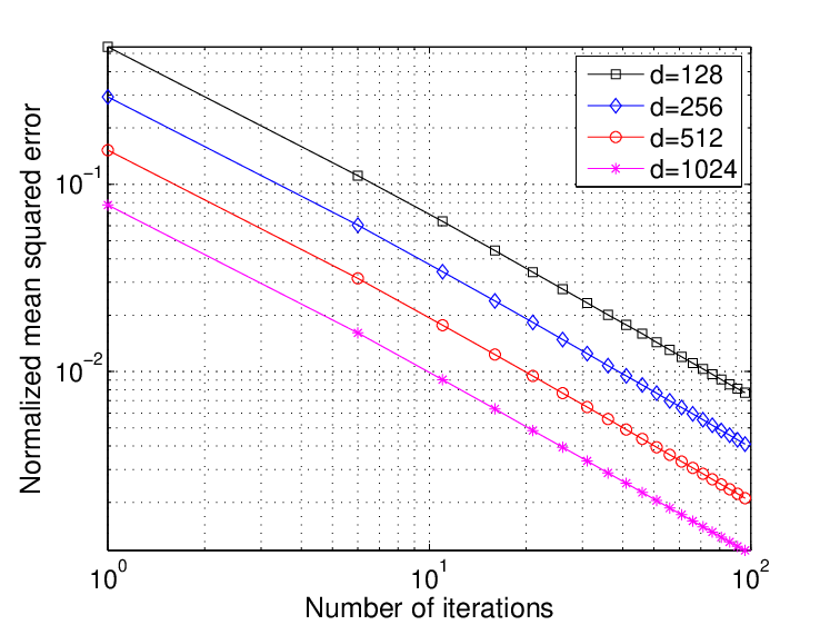
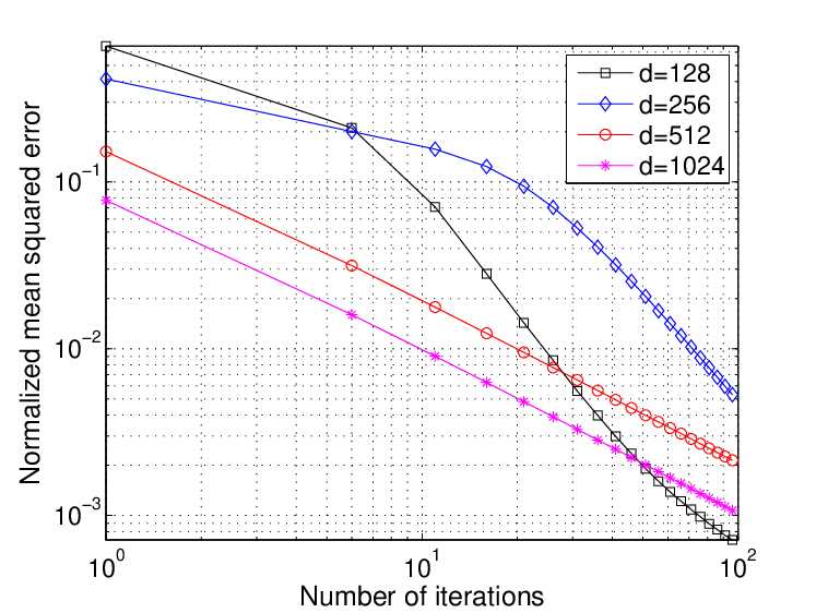
Our next set of simulations are designed to study the effect of increasing of the state dimension on convergence rates. We performed simulations both for the chain with nodes, as well as a two-dimensional square grid with nodes. In all cases, we implemented the SBP algorithm with step sizes , and generated the node/edge potentials with parameters and respectively. In Figure 5, we plot the normalized mean-squared error (estimated by averaging over trials) versus the number of iterations for the chain in panel (a), and the grid in panel (b). Each panel contains four different curves, each corresponding to a choice of state dimension . For the given step size, Theorem 2 guarantees that the convergence rate should be () with the number of iterations . In the log-log domain plot, this convergence rate manifests itself as a straight line with slope . For the chain simulations shown in panel (a), all four curves exhibit exactly this behavior, with the only difference with increasing dimension being a vertical shift (no change in slope). For the grid simulations in panel (b), problems with smaller state dimension exhibit somewhat faster convergence rate than predicted by theory, whereas the larger problems () exhibit linear convergence on the log-log scale.
| Chain | BP (per iteration) | 0.0700 | 0.2844 | 2.83 | 18.0774 |
| SBP (per iteration) | 0.0036 | 0.0068 | 0.0145 | 0.0280 | |
| BP (total) | 0.14 | 0.57 | 5.66 | 36.15 | |
| SBP (total) | 0.26 | 0.27 | 0.29 | 0.28 | |
| Grid | BP (per iteration) | 0.1300 | 0.5231 | 5.3125 | 32.5050 |
| SBP (per iteration) | 0.0095 | 0.0172 | 0.0325 | 0.0620 | |
| BP (total) | 0.65 | 3.66 | 10.63 | 65.01 | |
| SBP (total) | 0.21 | 1.31 | 0.65 | 0.62 |
As discussed previously, the SBP message updates are less expensive by a factor of . The top two rows of Table 1 show the per iteration running time of both BP and SBP algorithms, for different state dimensions as indicated. As predicted by theory, the SBP running time per iteration is significantly lower than BP, scaling linearly in in contrast to the quadratic scaling of BP. To be fair in our comparison, we also measured the total computation time required for either BP or SBP to converge to the fixed point up to a -tolerance, with . This comparison allows for the fact that BP may take many fewer iterations than SBP to converge to an approximate fixed point. Nonetheless, as shown in the bottom two rows of Table 1, in all cases except one (chain graph with dimension ), we still see significant speed-ups from SBP in this overall running time. This gain becomes especially pronounced for larger dimensions, where these types of savings are more important.
5.2 Applications in Image Processing and Computer Vision
 |
 | |
| (a) | (b) | |
 |
 | |
| (c) | (d) |
In our next set of experiments, we study the SBP on some larger scale graphs and more challenging problem instances, with applications to image processing and computer vision. Message-passing algorithms can be used for image denoising, in particular, on a two dimensional square grid where every node corresponds to a pixel. Running the BP algorithm on the graph, one can obtain (approximations to) the most likely value of every pixel based on the noisy observations. In this experiment, we consider a image with gray-scale levels, as showin in Figure 6(a). We then contaminate every pixel with an independent Gaussian random variable with standard deviation , as shown in Figure 6(b). Enforcing the Potts model with smoothness parameter as the edge potential, we run BP and SBP for the total of and iterations respectively to obtain the refined images (see panels (c) and (d), respectively, in Figure 6). Figure 7 illustrates the mean squared error versus the running time for both BP and SBP denoising. As one can observe, despite smaller jumps in the error reduction, the per-iteration running time of SBP is substantially lower than BP. Overall, SBP has done a marginally better job than BP in a substantially shorter amount of time in this instance.1111 11 Note that the purpose of this experiment is not to analyze the potential of SBP (or for that matter BP) in image denoising, but to rather observe their relative performances and computational complexities.

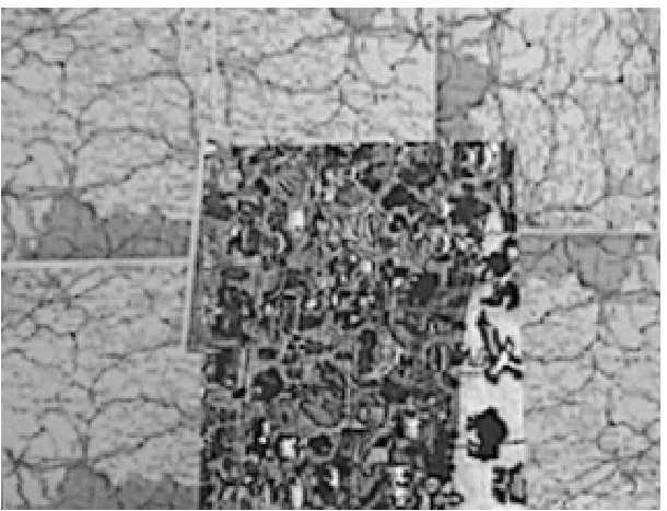
Finally, in our last experiment, we apply SBP to a computer vision problem. Graphical models and message-passing algorithms are popular in application to the stereo vision problem [28, 16], in which the goal is to estimate objects depth based on the pixel dissimilarities in two (left and right view) images. Adopting the original model in Sun et al. [28], we again use a form of the Potts model in order to enforce a smoothness prior, and also use the form of the observation potentials given in the Sun et al. paper. We then run BP and SBP (with step size ) for a total of and iterations respectively in order to estimate the pixel dissimilarities. The results for the test image “map” are presented in Figure 8. Here, the maximum pixel dissimilarity is , which makes stereo vision a relatively low-dimensional problem. In this particular application, the SBP is faster by about a factor of times per iteration; however, the need to run more iterations makes it comparable to BP. This is to be expected since the state dimension is relatively small, and the relative advantage of SBP becomes more significant for larger state dimensions .
 |
 |
| (a) | (b) |
 |
 |
| (c) | (d) |
6 Discussion
In this paper, we have developed and analyzed a new and low-complexity alternative to BP message-passing. The SBP algorithm has per iteration computational complexity that scales linearly in the state dimension , as opposed to the quadratic dependence of BP, and a communication cost of bits per edge and iteration, as opposed to real numbers for standard BP message updates. Stochastic belief propagation is also easy to implement, requiring only random number generation and the usual distributed updates of a message-passing algorithm. Our main contribution was to prove a number of theoretical guarantees for the SBP message updates, including convergence for any tree-structured problem, as well as for general graphs for which the ordinary BP message update satisfies a suitable contraction condition. In addition, we provided non-asymptotic upper bounds on the SBP error, both in expectation and in high probability.
The results described here suggest a number of directions for future research. First, the ideas exploited here have natural generalizations to problems involving continuous random variables and also other algorithms that operate over the sum-product semi-ring, including the generalized belief propagation algorithm [33] as well as reweighted sum-product algorithms [31]. More generally, the BP can be seen as optimizing the dual of the Bethe free energy function [33], and it would be interesting to see if SBP can be interpreted as a stochastic version of this Bethe free energy minimization. It is also natural to consider whether similar ideas can be applied to analyze stochastic forms of message-passing over other semi-rings, such as the max-product algebra that underlies the computation of maximum a posteriori (MAP) configurations in graphical models. In this paper, we have developed SBP for applications to Markov random fields with pairwise interactions. In principle, any undirected graphical model with discrete variables can be reduced to this form [33, 32]; however, in certain applications, such as decoding of LDPC codes over non-binary state spaces, this could be cumbersome. For such cases, it would be useful to derive a variant of SBP that applies directly to factor graphs with higher-order interactions. Finally, our analysis for general graphs has been done under a contractivity condition, but it is likely that this requirement could be loosened. Indeed, the SBP algorithm works well for many problems where this condition need not be satisfied.
Acknowledgements
Both authors were partially supported by MURI grant N00014-11-1-0688 to MJW. Both authors would like to thank Alekh Agarwal for helpful discussions on stochastic approximation and optimization at the initial phases of this research; the anonymous reviewers for their helpful feedback, as well as Associate Editor Pascal Vontobel for his careful reading and detailed suggestions that helped to improve the paper.
Appendix A Details of Example 1
In this appendix, we verify the sufficient condition for contractivity (24). Recall the definition (14) of the zero’th order bounds. By construction, we have the relations
Substituting these bounds into the definitions (22a) and (22b) and doing some simple algebra yields the upper bounds
where we have denoted the degree of the node by . Substituting these inequalities into expression (23) and noting that , we find that the global update function has Lipschitz constant at most
as claimed.
Appendix B Proof of Lemma 1
By construction, for each directed edge , the message vector belongs to the probability simplex—that is, , and . From equation (25), the vector is a convex combination of the columns of the matrix . Recalling bounds (14), we conclude that the message vector must belong to the set , as defined in equation (19), in particular with and . Note that the set is compact, and any member of it has strictly positive elements under our assumptions.
For directed edges and , let denote the Jacobian matrix obtained from taking the partial derivative of the update function with respect to the message vector . By inspection, the function is continuously differentiable; consequently, the function is continuous, and hence must achieve its supremum over the compact set . Consequently, we may use these Jacobian matrices to define a matrix with entries
We then use these matrices to define a larger matrix , consisting of sub-blocks each of size , with the
sub-blocks indexed by pairs of directed edges . In particular, the matrix occupies the sub-block indexed by the edge pair and . Note that by the structure
of the update function , the matrix
can be non-zero only if
and .
Now let denote the Jacobian matrix of the update function . By the integral form of the mean value theorem, we have the representation
Applying triangle inequality separately to each component of this -vector and then using the definition of , we obtain the elementwise upper bound
It remains to show that is nilpotent: more precisely, we show that is the all-zero matrix, where denotes the diameter of the graph . In order to do so, we first let be the “block indicator” matrix—that is, its entries are given by
Based on this definition, it is straightforward to verify that if
for some positive integer , then we also
have . Consequently, it suffices to show that
for .
Fix a pair of directed edges and , and some integer . We first claim that the matrix entry is non-zero only if there exists a directed path of length from to that includes both and , meaning that there exist nodes such that
We prove this claim via induction. The base case is true by construction. Now supposing that the claim holds at order , we show that it must hold at order . By definition of matrix multiplication, we have
In order for this entry to be non-zero, there must exist a directed
edge that forms a -directed path to
, and moreover, we must have , and . These conditions are
equivalent of having a directed path of length from
to , with and as intermediate
nodes, thereby completing the proof of our intermediate claim.
Finally, we observe that in a tree-structured graph, there can be no directed path of length greater than . Consequently, our intermediate claim implies that for any tree-structured graph, which completes the proof.
Appendix C Proof of Lemma 2
Appendix D Proof of Lemma 3
Let denote the Jacobian matrix of the function evaluated at . Since is differentiable, we can apply the integral form of the mean value theorem to write . From this representation, we obtain the upper bound
showing that it suffices to control the quantity .
Let be the matrix of partial derivatives of the function obtained from taking the partial derivatives with respect to the message vector . We then define a -dimensional matrix with the entries
| (47) |
Our next step is to show that . Let be an arbitrary -dimensional vector, where each sub-vector is an element of . By exploiting the structure of and , we have
where the bound (i) follows by triangle inequality; the bound (ii) follows from definition of the operator norm; and the final inequality (iii) follows by definition of .
Defining the vector with the entries , we have established the upper bound , and hence that
where the final equality uses the fact that by construction. Since both the message
and vector were arbitrary, we have shown that , as claimed.
Our final step is to control the quantities that define the entries of . In this argument, we make repeated use of the elementary matrix inequality [11]
| (48) |
valid for any matrix.
Recall the definition of the probability distribution (10) that defines the function , as well as our shorthand notation . Taking the derivatives and performing some algebra yields
for , and . For , we have
Putting together the pieces leads to the upper bounds
Recalling the definitions (22a) and (22b) of and respectively, we find that
Thus, by applying inequality (48) with , we conclude that
Since this bound holds for any message , we conclude that each of the matrix entries satisfies the same inequality. Again applying the basic matrix inequality (48), this time with , we conclude that is upper bounded by
which concludes the proof.
References
- [1] R. P. Agarwal, M. Meehan, and D. O’Regan. Fixed Point Theory and Applications. Cambridge University Press, 2004.
- [2] S. M. Aji and R. J. McEliece. The generalized distributive law and free energy minimization. In Allerton Conference on Communication, Control, and Computing, October 2001.
- [3] M. S. Arulampalam, S. Maskell, N. Gordon, and T. Clapp. A tutorial on particle filters for online nonlinear/non-Gaussian Bayesian tracking. IEEE Transaction on Signal Processing, 50(2):174–188, 2002.
- [4] A. Benveniste, M. Metivier, and P. Priouret. Adaptive Algorithms and Stochastic Approximations. Springer-Verlag, New York, NY, 1990.
- [5] F. Chung and L. Lu. Concentration inequalities and martingale inequalities: A survey. Internet Mathematics, 3(1):79–127, 2006.
- [6] J. Coughlan and H. Shen. Dynamic quantization for belief propagation in sparse spaces. Computer Vision and Image Understanding, 106(1):47–58, 2007.
- [7] A. Doucet, N. de Freitas, and N. Gordon. Sequential Monte Carlo methods in practice. Springer, New York, 2001.
- [8] R. Durrett. Probability: Theory and Examples. Duxbury Press, New York, NY, 1995.
- [9] P. F. Felzenszwalb and D. P. Huttenlocher. Efficient belief propagation for early vision. International Journal of Computer Vision, 70(1):41–54, 2006.
- [10] R. G. Gallager. Low-density parity check codes. MIT Press, Cambridge, MA, 1963.
- [11] R. A. Horn and C. R. Johnson. Matrix Analysis. Cambridge University Press, Cambridge, 1985.
- [12] A. T. Ihler, J. W. Fisher, and A. S. Willsky. Loopy belief propagation: Convergence and effects of message errors. Journal of Machine Learning Research, 6:905–936, May 2005.
- [13] A. T. Ihler and D. McAllester. Particle belief propagation. In Proceedings Conference on Artificial Intelligence and Statistics, pages 256–263, 2009.
- [14] M. Isard, J. MacCormick, and K. Achan. Continuously-adaptive discretization for message-passing algorithms. In Proceedings Advances in Neural Information Processing Systems (NIPS), pages 737–744, 2009.
- [15] K. Kersting, B. Ahmadi, and S. Natarajan. Counting belief propagation. In Proceedings Twenty-Fifth Conference on Uncertainty in Artificial Intelligence, 2009.
- [16] A. Klaus, M. Sormann, and K. Karner. Segment-based stereo matching using belief propagation and a self-adapting dissimilarity measure. In Proceedings 18th International Conference on Pattern Recognition, pages 15–18, 2006.
- [17] F. R. Kschischang, B. J. Frey, and H. A. Loeliger. Factor graphs and the sum-product algorithm. IEEE Transaction on Information Theory, 47(2):498–519, 2001.
- [18] H. A. Loeliger. An introduction to factor graphs. IEEE Signal Processing Magazine, 21:28–41, 2004.
- [19] J. J. McAuley and T. S. Caetano. Faster algorithms for max-product message passing. Journal of Machine Learning Research, 12:1349–1388, 2011.
- [20] J. M. Mooij and H. J. Kappen. Sufficient conditions for convergence of the sum-product algorithm. IEEE Transactions on Information Theory, 53(12):4422–4437, December 2007.
- [21] A. C. Rapley, C. Winstead, V. C. Gaudet, and C. Schlegel. Stochastic iterative decoding on factor graphs. In Proceedings 3rd International Symposium on Turbo Codes and Related Topics, pages 507–510, 2003.
- [22] H. Robbins and S. Monro. A stochastic approximation method. Annals of Mathematical Statistics, 22:400–407, 1951.
- [23] T. G. Roosta, M. J. Wainwright, and S. S. Sastry. Convergence analysis of reweighted sum-product algorithms. IEEE Transactions on Signal Processing, 56(9):4293–4305, September 2008.
- [24] H. L. Royden. Real Analysis. Prentice-Hall, New Jersey, 1988.
- [25] H. Song and J. R. Cruz. Reduced-complexity decoding of q-ary ldpc codes for magnetic recording. IEEE Transaction on Magnetics, 39(2):1081–1087, 2003.
- [26] L. Song, A. Gretton, D. Bickson, Y. Low, and C. Guestrin. Kernel belief propagation. In Proceedings Artificial Intelligence and Statistics (AISTATS), 2011.
- [27] E. B. Sudderth, A. T. Ihler, W. T. Freeman, and A. S. Willsky. Nonparametric belief propagation. In Proceedings IEEE Conference on Computer Vision and Pattern Recognition, volume 1, pages 605–612, 2003.
- [28] J. Sun, H. Y. Shum, and N. N. Zheng. Stereo matching using belief propagation. IEEE Transactions on Pattern Analysis and Machine Intelligence, 25(7):787–800, 2003.
- [29] S. Tatikonda and M. I. Jordan. Loopy belief propagation and Gibbs measures. In Proc. Uncertainty in Artificial Intelligence, volume 18, pages 493–500, August 2002.
- [30] S. S. Tehrani, W. J. Gross, and S. Mannor. Stochastic decoding of ldpc codes. IEEE Communications Letters, 10(10):716–718, 2006.
- [31] M. J. Wainwright, T. S. Jaakkola, and A. S. Willsky. A new class of upper bounds on the log partition function. IEEE Trans. Info. Theory, 51(7):2313–2335, July 2005.
- [32] M. J. Wainwright and M. I. Jordan. Graphical Models, Exponential Families, and Variational Inference. Now Publishers Inc, Hanover, MA 02339, USA, 2008.
- [33] J. S. Yedidia, W. T. Freeman, and Y. Weiss. Constructing free energy approximations and generalized belief propagation algorithms. IEEE Transaction on Information Theory, 51(7):2282–2312, July 2005.