Elements of a theory for multiparton interactions in QCD
Abstract
We perform a detailed investigation of multiple hard interactions in hadron-hadron collisions. We discuss the space-time, spin and color structure of multiple interactions, classify different contributions according to their power behavior and provide several elements required for establishing all-order factorization. This also allows us to analyze the structure of Sudakov logarithms in double hard scattering. We show how multiparton distributions can be constrained by connecting them with generalized parton distributions and by calculating their behavior at large transverse parton momenta.
1 Introduction
When two hadrons collide at high energies, more than one parton in one hadron can have a hard interaction with a parton in the other hadron and produce particles with large mass or transverse momentum. The effects of such multiparton interactions are suppressed or average out in sufficiently inclusive observables, but they have important consequences for the details of the hadronic final state. The possible importance of multiparton interactions has been realized long ago [1, 2] and phenomenological estimates have been given for many final states such as four jets (possibly including quarks) [3, 4, 5, 6, 7, 8, 9], jets associated with photons or leptons [10], four leptons produced by the double Drell-Yan process [11, 12, 13] or from two charmonium states [14, 15, 16], as well as a number of channels with electroweak gauge bosons [17, 18, 19, 20, 21, 22, 23, 24, 25, 26]. Experimental evidence for multiple hard scattering has been found in the production of multijets [27, 28, 29] and of a photon associated with three jets [30, 31, 32, 33]. A mini-review of the subject can be found in [34] and an overview of how multiparton interactions are modeled in current Monte Carlo event generators is given in [35].
At LHC energies, the phase space for having several hard interactions in a proton-proton collision is greatly increased compared with previous experiments, and it is expected that the effects of multiple interactions will be important in many processes [36, 37, 38, 39]. This poses a challenge in searches for new physics and at the same time offers the possibility to study multiple interactions in much more detail than before. First experimental results on multiple hard scattering at the LHC have already appeared [40] and more can be expected in the near future [41].
Understanding multiparton interactions is also important for heavy-ion physics, where or proton-nucleus collisions are used as a baseline for collective effects in nucleus-nucleus collisions. Compared with collisions, multiparton interactions with nuclei have the additional feature that the different scattering partons may come from the same nucleon or from different nucleons in the nucleus. Dedicated investigations of multiple interactions in collisions can be found in [42, 43, 44, 45, 46].
Phenomenological estimates of multiparton interactions, as well as their implementation in event generators, are based on a rather simple and physically intuitive picture, whose basic ingredient is the probability to find several partons inside a proton. On the other hand, a systematic description of multiparton interactions in QCD has not been achieved so far. In the present work, we present a number of steps in this direction. A brief account of our main results has been given in [47]. We require all parton-level scatters to have a hard scale, so that the concepts of hard-scattering factorization and of parton distributions can be applied. Since transverse momenta of final-state particles play a crucial role in the characterization of multiple interactions, we fully keep track of this degree of freedom and base our discussion on transverse-momentum dependent multiparton distributions.
In section 2 we give a lowest-order analysis of multiple hard scattering. We find that the intuitive picture just mentioned emerges for a subset of all relevant contributions to the cross section, but that there are other contributions which may be of comparable size and hence call for further investigation. In section 3 we take first steps to extend existing factorization theorems for single-hard scattering processes with measured transverse momentum [48, 49, 50, 51] to the case of multiple hard scattering. While many ingredients for a full proof of factorization are still missing (and the possibility that factorization is broken cannot be ruled out), we obtain a number of encouraging results that allow us in particular to analyze the structure of Sudakov logarithms. Section 4 gives more details about the distribution of two quarks or antiquarks in the proton, in particular about the effects of spin correlations and the possibility to learn more about multiparton distributions by calculating their moments in lattice QCD or by linking them to generalized parton distributions. The predictive power of perturbation theory is increased in kinematics where all observed transverse momenta (as well as their vectors sums) are large on a perturbative scale. Complications and simplifications that arise in this regime are discussed in section 5, where we will also encounter the conceptual problem of separating single from multiple hard-scattering contributions in a systematic and consistent fashion. Section 6 contains our conclusions.
2 Lowest order analysis
2.1 Momentum and position space structure
In this section we investigate the structure of multiparton interactions in momentum and position space, restricting ourselves to graphs with the lowest order in the strong coupling. To avoid a clutter of indices we consider scalar partons described by a hermitian field , deferring the inclusion of spin and color degrees of freedom to sections 2.2 and 2.3. Our derivation of the cross section formula for multiparton interactions uses standard methods. For cross sections integrated over transverse momenta in the final state, similar derivations can be found in the literature [52, 53]. The extension to cross sections differential in transverse momenta is new. For ease of language we refer to the colliding hadrons as protons throughout this work, bearing in mind that our results apply without change to collisions or to any other hadron-hadron collision.
2.1.1 Definition of multiparton distributions
We begin by defining the multiparton distributions that appear in the cross section formula we will derive shortly. The following definitions need to be completed by a prescription to renormalize ultraviolet divergences and by Wilson lines that take into account collinear and soft gluons as required to achieve factorization for the cross section. These issues will be discussed in section 3.
The building block from which multiparton distributions can be defined is the parton correlation function
| (1) |
where denotes time-ordering and anti-time-ordering of the fields. This function describes the emission of partons in a scattering amplitude and in its complex conjugate. Throughout this work we assume an unpolarized target: if the target carries spin then an average over its polarization is implicit in (1) and all subsequent expressions. The parton four-momenta in the correlation function are subject to the constraint
| (2) |
In (1) we have chosen the position of the first field in the matrix element to be . Taking this position as arbitrary and integrating over it with a factor yields a delta function for the constraint (2). The structure of the cross section will be more transparent if we use symmetric variables
| (3) |
The constraint (2) then turns into
| (4) |
and we can rewrite the correlation function (1) as
| (5) |
where we have replaced using (4). In addition we have used translation invariance to shift position arguments in the matrix element by . Substituting position variables according to
| (6) |
and , we obtain
| (7) |
The assignment of momentum and position arguments is shown in figure 1.

We now introduce light-cone coordinates and for any four-vector . In a frame where we define multiparton distributions
| (8) |
This can be written as
| (9) |
where we have used the abbreviation
| (10) |
for the bilinear parton operators and traded the factors for derivatives acting on the fields. When going from (8) to (9) we have replaced the time- or anti-time-ordered products appearing in (7) by usual products, which are understood to be normal ordered. To justify this it is crucial that the arguments of all fields in the operators (10) have a vanishing plus-component. For a generic configuration with all and different from zero and from each other, all fields in (10) have a spacelike separation, so that they commute because of causality and can be written in any order. The case where fields have a lightlike separation requires special treatment, and different methods for this case have been used in the literature for related matrix elements, see [54, 55] and [56]. As we shall see in section 5, lightlike field separations in (9) also lead to divergences that need to be regulated.
We also introduce distributions that depend partially or entirely on transverse positions ( and ) instead of transverse momenta ( and ):
| (11) |
and
| (12) |
In the arguments of (11) and (12) it is understood that the average transverse position of the first two field operators is . The three forms (9), (11) and (12) can be used interchangeably, and each of them has advantages in different situations. As we shall see, the momentum representation (9) naturally appears in Feynman graph calculations, the mixed representation (11) has a rather simple physical interpretation, and the position space representation (12) is most convenient for the discussion of Sudakov logarithms.
The factors of , , and in (8) to (12) have been chosen such that the collinear (i.e. transverse-momentum integrated) distribution
| (13) | ||||
| as well as the distribution | ||||
| (14) | ||||
admit a probability interpretation. is the probability to find partons with plus-momentum fractions and transverse distances from parton number , and is the probability to find partons with plus-momentum fractions and transverse momenta .
By contrast, is not a probability (due to the uncertainty relation one cannot simultaneously fix transverse momentum and transverse position) but rather has the structure of a Wigner distribution [57] in the transverse variables. Its integral over all gives the probability to find partons at transverse positions , and its integral over all gives the probability to find partons with transverse momenta . A related interpretation for generalized parton distributions can be found in [58]. In figure 1 we can identify as the “average” transverse momenta of the partons and as their “average” transverse position, where the “average” is taken between the partons to the left and to the right of the final-state cut in the figure. In a physical process, this corresponds to an average between partons in the scattering amplitude and its complex conjugate.
The interpretation of multiparton distributions becomes more explicit if one represents them in terms of the light-cone wave functions of the target, see [59]. Most conveniently derived in the framework of light-cone quantization, this representation is analogous to the wave function representation for single-parton densities [60] and generalized parton distributions [61, 62]. The distributions in (13) and (14) can be written in terms of squared wave functions in impact parameter or transverse-momentum space, which makes their probability interpretation manifest. The wave function representation also offers a way to model multiparton distributions in the region of large momentum fractions, where one can expect a small number of partonic Fock states to be dominant. We shall not pursue this avenue in the present work.
In later chapters we will also need collinear distributions that depend on the momentum transfer variables ,
| (15) |
We will see in the following section that or equivalently appear in multiple-scattering cross sections. This is not the case for the distributions
| (16) |
which give the probability to find partons with momentum fractions and unspecified transverse positions or transverse momenta. We note that the integrals over in (13), (15) and (16) are logarithmically divergent and require appropriate regularization, which will be discussed in sections 5.1.2 and 5.3.2.
The definitions in this section are given for right-moving partons, with being plus-momentum fractions. Analogous definitions for left-moving partons are obtained by exchanging the plus- and minus-components of all position and momentum vectors.
2.1.2 Cross section for hard scatters
We now evaluate the cross section for a process with scatters at parton level, as sketched in figure 2. We work in a reference frame with and consider kinematics where the squared c.m. energy of each scatter is large and where each transverse momentum is much smaller than and . Defining
| (17) |
we can then approximate
| (18) |
where is the squared overall c.m. energy. We neglect the target mass throughout, so that and the flux factor in the cross section is . One can trade the momentum fractions and for and the rapidities
| (19) |
with
| (20) |
where we have again used (18). We note that for the very high achieved at the LHC, both and are rather small, except if or is very large.

The cross section for hard scatters is given by
| (21) |
where the combinatorial factor contains a factor for each set of identical hard-scattering final states.11 1 An often used notation for two hard scatters is to write in the place of , with if the hard-scattering final states are identical and if they are distinct. The remnant of proton () consists of () spectators with momenta (). denotes the squared matrix element for the th hard scatter, with truncated propagators of the incoming parton lines. includes integration over the internal phase space of the final state produced by the hard scatter, with only the four-momentum kept fixed. If such a final state is the decay product of a single particle with mass and width (e.g. a or a Higgs boson) then includes a factor
| (22) |
which in the limit of narrow width constrains to be on the mass shell. If the final state is a stable single particle with mass , then includes a delta function
| (23) |
so that together with the integration element in (21) one obtains the correct one-particle integration measure . We now rewrite the cross section in terms of the correlation functions (1). To this end we use
| (24) |
Using the analogous relation for the matrix element between and and rewriting the momentum conservation constraint in (21) as
| (25) |
we can express the cross section as
| (26) |
where in the last step we have switched to the set of symmetric variables (3). They have the important property that the kinematic constraints on and do not involve the final-state momenta , which will lead to a great simplification below.
Hard-scattering approximation.
The parton-level scattering processes involve a hard scale, which we collectively denote by without assuming a particular hierarchy among the individual squared momenta . The case where one of them is much larger than the others is of particular relevance for the description of the underlying event, but we shall not investigate the consequences of such a hierarchy in the present work. In the graph of figure 2 it is understood that partons emerging from the shaded blobs have virtualities much smaller than . The components of the various four-momenta thus scale like
| (27) |
and
| (28) |
where denotes the size of the transverse momenta or the scale of non-perturbative interactions, whichever is larger. The momentum conservation constraint enforces that the components
| (29) |
are small, although by general scaling arguments they could be of order . The constraint leads to
| (30) |
up to relative corrections of order . We make these approximations in the correlation functions and and see that the longitudinal momenta of the partons entering the hard scattering are fixed by the final-state kinematics. In the squared hard-scattering matrix element we can neglect all transverse momenta and all components of order . With (30) this only leaves a dependence on the independent variables and . Since is invariant under a boost along the axis, it can then only depend on . Altogether we then have
| (31) |
Inserting this into the cross section (26) and using the definition (8) of the multiparton distributions gives
| (32) |
Rewriting , we obtain our final result for the cross section in momentum representation,
| (33) |
where we have introduced the cross section
| (34) |
for the th parton-level subprocess and used the approximation (18). We have carried out the integrations over using the constraints , so that the distributions for the two protons are evaluated at opposite values of their last arguments. Fourier transforming these to position space, we have
| (35) |
and the distributions are evaluated at equal values of . Transforming also the arguments and , we have
| (36) |
where all position arguments in the two distributions coincide.
The interpretation of the distributions discussed in section 2.1.1 extends to the cross section formula (35). In each individual hard subprocess, two partons with average transverse momenta and produce a final state with transverse momentum . The th scatter occurs at an average transverse distance from the th scatter. The hard scatters are approximated to be local in transverse space, so that their average distance is equal to the average distance between the colliding partons in each proton. We thus find a rather intuitive interpretation of the variables in our cross section formula, provided that we “average” the transverse momenta and positions between the amplitude and its conjugate. Let us however emphasize that we have obtained (35) from calculating Feynman graphs using standard hard-scattering approximations, without any appeal to classical or semi-classical arguments.
Integrating the cross section over all transverse momenta we obtain a simple result
| (37) |
in terms of collinear multiparton distributions. This formula has long been known and provides the basis of most phenomenological analyses of multiple interactions in the literature. It was derived in [52] for scalar partons in a way very similar to the one we have employed here.
2.1.3 Single vs. multiple hard scattering
The approximations we have made in the previous section give the leading term of an expansion in powers of . Let us investigate how the resulting cross section (35) scales with . As can readily be seen from its definition (11), the mass dimension of is and one has . To obtain this power behavior, it is essential that the distribution is invariant under a boost along the axis. For instance, a hadronic matrix element that transforms like the plus-component of a vector would be proportional to or another large plus component and thus scale like times the appropriate power of . Note that the dependence of on the large scale via renormalization group or Sudakov logarithms (see section 3) is neglected at the level of power counting. The hard-scattering cross sections have a power behavior , and the integrations over transverse momenta count as . Finally, the distances in (35) are generically of size so that . Putting all ingredients together, one finds
| (38) |
for the cross section of hard scatters. One obtains of course the same result if the power counting is done for the representations (33) in momentum space or (36) in position space, using or .
Let us compare this with the cross section for producing the final states with momenta in a single hard scattering. With
| (39) |
the factorization formula for this case reads
| (40) |
where is the appropriate hard-scattering cross section and and are transverse-momentum dependent single-parton densities. The definition of can be obtained from (11) by setting , which gives a power behavior . We now make (40) differential in the internal momentum variables of the final state, which we choose as
| (41) |
and with . We then have
| (42) |
The differential hard-scattering cross section on the r.h.s. behaves as , so that we have
| (43) |
We obtain the important result that if one leaves the cross section differential in the transverse momenta , the contributions from single and from multiple hard scattering have the same power behavior in the large scale , so that multiple hard scattering is not power suppressed. It is easy to see that the power behavior in (38) and (43) holds for any combination of single and multiple hard scatters, e.g. when producing the final states with momenta and in a single hard scatter and each final state with momentum , , etc. in a hard scatter of its own.
Let us now see what happens if we integrate over the . In the multiple-scattering mechanism, each transverse momentum is the sum of two parton momenta and thus limited to be of size , so that the phase space volume is . With a single hard scattering, however, the individual momenta can be as large as the hard scale , and only their sum is limited to be of order by the constraint in (42). The phase space volume in this case is therefore , and we have
| (44) |
for the cross sections integrated over all transverse momenta. Multiple-scattering contributions are now suppressed by at least one power of and are hence power corrections to the contribution from a single hard scattering, as has been known for a long time [63]. This is indeed necessary for the validity of the familiar collinear factorization theorems, which only take into account single hard scatters.
Power counting in the hard scale provides an essential criterion for determining which contributions to the cross section are important. There are, however, other important factors to keep in mind. We already mentioned Sudakov logarithms in , which appear in the cross section differential in and are different for single and multiple hard scattering. They will be discussed in section 3.4. Another aspect in which single and multiple scattering contributions differ is the dependence on the momentum fractions and , which can be rather small as we remarked after (20). We will return to this point in section 2.4.
2.1.4 Impact parameter representation
The cross section in (36) involves distributions that depend on the transverse positions of the scattering partons but still refer to proton states with definite (zero) transverse momenta. In this section we give a formulation completely in transverse position space, closely following the construction of impact-parameter dependent parton distributions in [64, 65, 62].
To begin with, we define a non-forward correlation function exactly as in (1) but with a state having a different momentum than the state . Using the same arguments as in section 2.1.1 we can derive a representation of the form (7) for , with replaced by . The constraints on the parton momenta read
| (45) |
in this case. In the same manner we define multiparton distributions , and as in (8) to (12), but taken between states and . Note that we take the same plus-momentum in the bra and ket state, even if their transverse momenta are different.
We now consider a transverse boost, i.e. a Lorentz transformation that changes the transverse components of a four-vector as
| (46) |
and leaves plus-components unchanged. Invariance under this transformation implies
| (47) |
with
| (48) |
In impact parameter space we then have
| (49) |
We now introduce proton states with definite impact parameter:
| (50) |
One readily obtains their normalization
| (51) |
from the usual relativistic normalization of momentum eigenstates (recall that at fixed one has in the invariant integration element). For later use we also give the projector on one-particle states,
| (52) |
which is readily checked by taking the matrix element between the one-particle states in (50) and using (51). We finally define the center of momentum of particles with plus-momenta and transverse positions as
| (53) |
By virtue of Lorentz invariance, this is a conserved quantity. Note the analogy between (46) and non-relativistic boosts if is a momentum and if one replaces plus-momenta by masses. The center of momentum is thus the analog of the center of mass in the non-relativistic case, which is of course conserved.
Let us consider the matrix element of the same operator as in (12), but taken between impact parameter instead of transverse-momentum eigenstates. We have
| (54) |
The delta function in the last line reflects the conservation of the center of momentum, which equals
| (55) |
for the bra and ket states in the matrix element, respectively. Here and is the center of momentum of the spectator partons. We define impact-parameter dependent multiparton distributions by
| (56) |
If we set then the matrix element in (54) is taken at and hence becomes diagonal. We can interpret as the probability to find partons with plus-momentum fractions in a target that is localized in impact parameter space, with parton number at a transverse distance from the center of the target and partons to at relative transverse distances from parton .
Inverting (56) and setting we get
| (57) |
and can therefore represent the multiple-scattering cross section (36) as
| (58) |
Integration over leads to as in (37). The resulting cross section formula was already derived in [66], and it has a very intuitive geometric interpretation shown in figure 3. As already noted after (36), the approximations we have made for the hard-scattering subprocesses imply that each pair of colliding partons in the hadrons and must be at the same position in impact parameter space. The relative distances between the partons are hence the same in both hadrons, but the distance of the partons from the center of their parent hadron is in general different in and . The relative transverse distance between the hadrons is integrated over in the cross section.

Our result (58) shows that the representation of the cross section in terms of impact-parameter dependent distributions remains simple even if the transverse momenta are kept fixed. In the geometric interpretation just described, we then have to replace “distances” by “average distances”, with the average taken between the amplitude and its conjugate. What is lost in this case is a probability interpretation of the multiparton distributions. The two fields associated with a parton in the target are now taken at a relative transverse distance , whose typical size is .
2.1.5 Reduction to single-parton distributions
In order to build a phenomenology of multiple interactions, one needs a simple ansatz for multiparton distributions as a starting point. It is natural to approximate those distributions that have a probability interpretation by the product of single-parton densities. In this section we show how one can formally implement this approximation and generalize it to the distributions or , which do not represent probabilities.
To this end we insert complete sets of intermediate hadron states in the operator product appearing in the multiparton distributions:
| (59) |
Note that the two parton fields in each operator are associated with the same plus-momentum fraction in the multiparton distributions.
The approximation that gives a product of single-parton distributions is to assume that among all intermediate states the dominant ones are single-proton states. This reduces the complete sets of intermediate states to the projection operators (52), and one obtains
| (60) |
Translation invariance and the definition (50) of impact-parameter states imply
| (61) |
and hence
| (62) |
Using (54) for , we have
| (63) |
where can be written as
| (64) | ||||
| with | ||||
| (65) | ||||
A reader familiar with generalized parton distributions will recognize that
| (66) |
is a transverse-momentum dependent generalized parton distribution at zero skewness. We will shortly need the collinear distributions
| (67) |
as well. Introduced long ago in [64, 65], the impact parameter density gives the probability to find a parton with momentum fraction at a transverse distance from the center of the proton.
The delta function on the r.h.s. of (63) implies that
| (68) |
in (62), so that we obtain the desired approximation
| (69) |
of a multiparton distribution. Setting and integrating over , we obtain in particular the collinear multiparton distribution in terms of impact-parameter dependent single-parton densities,
| (70) |
This relation is illustrated in figure 4, which uses the representation of parton distributions as squared light-cone wave functions we mentioned briefly before (15).

Let us now insert (69) into the cross section (58). For measured transverse momenta , the different single-parton distributions are entangled by their dependence. By contrast, the integrated cross section simplifies to
| (71) |
where the only integration variable linking the different factors is the relative distance , and where we have renamed the integration variable to in the second step. In different forms, this relation (or more precisely its analog for quarks and gluons instead of scalar partons) has long been used as a starting point of phenomenological studies, see e.g. [67, 68, 69, 70, 71] and [72, 8].22 2 We note that in [72, 8] the impact parameter arguments of are and instead of and (if we translate to our notation). This is equivalent in the spin independent sector, where the single-parton distributions are independent of the direction of the impact parameter.
As observed in [59] for the case of collinear distributions, the reduction of multiparton to single-parton distributions also takes a simple form in the transverse-momentum representation. This remains true if one keeps the transverse parton momenta unintegrated. To see this, we integrate (69) over and Fourier transform w.r.t. and as specified by (11) and (12). Changing integration variables from and to the impact parameter arguments of the distributions on the r.h.s. of (69), we obtain
| (72) |
where we recall that . Integrated over the momenta this simply reads
| (73) |
so that the cross section (71) becomes
| (74) |
The arguments in (73) can easily be anticipated from figure 1.
We emphasize that the relations (69) to (73) have been obtained by restricting a sum over all intermediate states to a single proton. We do not have a motivation for this restriction other than observing that it results in neglecting correlations between different partons in the proton. It seems plausible to assume that this is a reasonable first approximation, at least in a certain region of variables, but one should not expect it to be very precise. Possible deviations from this approximation and their phenomenological consequences have recently been discussed in [73, 74, 75, 76, 8, 77].
2.2 Parton spin
Let us now see how the scattering formulae (33) to (37) are modified in QCD, where partons have nonzero spin. In (21) to (31) the squared amplitude of the th hard scattering and the hadronic matrix elements of parton field operators acquire spinor indices in the case of quarks and Lorentz indices in the case of gluons. These indices can be treated as in the case of a single hard scattering. For the time being we still omit color degrees of freedom, which will be discussed in section 2.3.
2.2.1 Quarks
The correlation function for quarks entering the hard scattering is
| (75) |
When this is integrated over the parton minus-momenta, the anti-time and time ordering can be omitted and one can reorder the fields as
| (76) |
by an even permutation. For antiquarks entering the scattering, one has an operator product instead of .
Consider the case of a quark entering the hard scattering. We wish to rearrange the spinor indices in the product , where for brevity we write instead of and leave out all other indices on which and depend. The rearrangement is achieved by the Fierz transform
| (77) |
The Dirac matrices with open indices on the r.h.s. multiply fields in the correlation function for the right-moving proton. The dominant terms in the cross section are those where that matrix is or with , because is then proportional to the large momentum component by virtue of Lorentz invariance. The traces over the hard scattering matrix on the r.h.s. of (77) have both large plus and minus components since depends on the boson momentum . One thus has
| (78) |
where a sum over the transverse index is understood.
When defining distributions for scalar partons in (8), we included a factor for each parton . For quarks we do not do this, but instead include this factor in the definition of the parton-level cross section from the squared matrix element . Writing for the collinear approximation of (i.e. , and ) we recognize in
| (79) |
the spin averaged squared amplitude for an incoming on-shell quark. The corresponding terms with and are respectively associated with scattering on a longitudinally and transversely polarized quark.
Integrating (75) over the minus components of the parton momenta, one obtains multi-parton distributions as in (9) with the scalar field operators (10) replaced by quark bilinears
| (80) |
where labels the polarization and
| (81) |
We recognize the operators that appear in the definition of single-parton densities for unpolarized, longitudinally polarized and transversely polarized quarks, see e.g. [78, 79]. For antiquarks entering the hard scattering one proceeds in an analogous way. The corresponding operators are
| (82) |
with
| (83) |
The overall minus sign in (82) reflects a change in the order of field operators from to , cf. our remark after (76). In the case of a further minus sign is included in , so that the operator corresponds to the difference of antiquarks with positive and negative helicity.

From now on we concentrate on two-parton distributions. The formalism can be extended without conceptual difficulties to higher multiple interactions, but the resulting expressions become rather unwieldy. As one encounters nontrivial features already for double hard scattering, it is natural to elaborate this case first. To simplify the discussion, we introduce a compact notation
| (84) |
for the Fourier transformed matrix element of a product of field operators . Their indices are assigned according to
| (85) |
as shown in figure 5. Throughout this paper we consider unpolarized incident hadrons, so that an average over the proton spin is understood in (84). A two-quark distribution is then given by
| (86) |
and if the parton with momentum fraction is an antiquark one has instead
| (87) |
In straightforward extension of the case of single-parton distributions [79], the matrix elements defining distributions for quarks and antiquarks are thus connected as
| (88) |
with sign factors and . Definitions and relations analogous to (86), (87) and (88) hold for the case where the parton with momentum fraction is an antiquark.
The previous arguments can be repeated for the partons in the left-moving proton, with the roles of plus and minus components interchanged. We define the hard-scattering cross section for a right-moving quark and a left-moving antiquark as
| (89) |
with spin projectors
| (90) | |||||||
constructed from the collinear momenta introduced before (79), i.e. for right-moving partons and for left-moving ones, with all other components equal to zero. The spin projectors match the Fierz decomposition (78) and the operators in (80) and (82), and they can be expressed in terms of quark or antiquark spinors as in (79). It is understood that for each label or the cross section (89) depends on a transverse Lorentz index, which has not been explicitly displayed. In most reactions the partonic subprocess involves only chirality conserving interactions. Since incoming quarks and antiquarks are approximated as massless in the hard scattering, only the combinations , , , and are then nonzero. For parity conserving processes such as the production of a virtual photon, one is left with only , and . Hard-scattering cross sections for right-moving antiquarks and left-moving quarks are defined as in (89) with an appropriate change of spinor indices.

We now have everything at hand to write down the expression for the double-scattering graphs of figure 6a and b. For a single quark flavor, one has
| (91) |
where if the final states of the two hard scatters are identical and otherwise. It is straightforward to Fourier transform the previous expressions either from the interparton distance to the relative transverse momentum , or from average transverse momenta to transverse positions , as we did in (9), (12) and (33), (36) for scalar partons.
Notice that (91) involves a polarization dependence in the multiparton distributions and hard-scattering cross section. This is because, even for unpolarized hadron beams, the polarization of the two partons with momentum fractions and can be correlated among themselves. We will discuss this in more detail in section 4.1.1.
The two-quark and quark-antiquark distributions considered so far have the form , where the are bilinear operators from (80) or (82). As we discussed after (14), these distributions can be interpreted as probabilities or pseudo-probabilities in the sense of Wigner distributions for two partons in the proton that carry momentum fractions and , respectively.
There are further double-scattering graphs that contribute to the cross section and involve distributions which represent interference terms rather than probabilities. In figure 6c we show the case where the parton with momentum fraction is a quark in the scattering amplitude and an antiquark in the conjugate scattering amplitude. Such interference terms in fermion number have no equivalent in single hard-scattering processes, where they are forbidden by fermion number conservation. For their description we introduce interference distributions
| (92) |
In the absence of a probability interpretation, the choice of quark vs. antiquark labels in the Dirac matrices is pure convention. We assign labels such that indicates a quark and an antiquark in the amplitude, i.e. for the parton indices 1 and 2 in figure 5. The graph in figure 6c contributes to the cross section as
| (93) |
We see that the contraction of Dirac indices ties together the two hard-scattering kernels and the spin projectors , so that one cannot define separate partonic cross sections and . The power behavior of this contribution is the same as in (91).

Taking different quark flavors into account, we obtain further interference terms. The contributions in figure 7a and b involve the interference of different quark flavors, and those in figure 7c and d the combined interference in fermion number and flavor. The relevant matrix elements are easily written down, reading e.g. for the lower part of figure 7a.
Which interference distributions are of appreciable size is interesting from the point of view of nucleon structure and important for phenomenology. One may for instance imagine that diquark-like correlations in the nucleon wave function play an important role in this context. In section 2.5 we will argue that for small values of both fermion number and quark flavor interference distributions should become relatively small.
2.2.2 Gluons
If gluons enter a hard-scattering subprocess, special attention needs to be paid to their polarization. In covariant gauges such as Feynman gauge, an unlimited number of right-moving gluons with polarization in the plus direction can be attached to a hard scattering graph without any power suppression. The effect of these gluons is resummed into Wilson lines, which we will discuss in detail in section 3.2.1. Alternatively, one may work in light-cone gauge , where the corresponding gluon polarization is absent. One then has to be careful about subtle effects from Wilson lines at infinity, see our remark at the end of section 3.2.1.
Once the right-moving gluons with plus polarization (and the left-moving gluons with minus polarization) are taken into account, the leading contribution to the cross section comes from gluons with transverse polarization, corresponding to field operators with . It is for these gluons that one introduces parton distributions similar to those of quarks. To decompose the product of two gluon potentials with transverse polarization, we use the relations
| (94) |
where the indices are restricted to be transverse and where is the two-dimensional antisymmetric tensor with . The tensor is symmetric and traceless in each of the index pairs and . As an analog of the decomposition (77) for fermions, we can thus write
| (95) |
for the squared hard-scattering matrix element, where in the last step we have used the relation .
The tensors depending on in (95) are to be contracted with a product of gluon potentials in the multigluon correlation function
| (96) |
In analogy to the definition (8) for scalar partons (and in contrast to the one for quarks) we include a factor for each gluon when defining multi-gluon distributions from . One then obtains
| (97) |
where
| (98) |
with polarization labels and
| (99) |
The operators and appear in the usual densities for unpolarized and longitudinally polarized gluons. By contrast, describes the interference of two gluons whose helicities differ by two units, or equivalently the difference between linear gluon polarization in two orthogonal directions. Such distributions have previously been discussed in different contexts, see [80, 81] and [82, 83, 84, 85, 86, 87].
In going from (96) to (97) we have traded gluon potentials for field strengths using the relation valid in the light-cone gauge . Under the Fourier transform this turns into and explains the factor for each parton in (97). It is plausible that gluon field strengths rather than potentials should appear in the definition of gluon distributions, since has a simple behavior under gauge transformations and can be used to construct gauge invariant operators. How a definition with emerges in Feynman gauge is rather involved and has been shown explicitly for the case of a single hard scattering in [88].
Parton-level cross sections for gluons are defined as in (89) with spin projectors
| (100) |
following from (95). In one readily recognizes the average over the two transverse gluon polarization. The expressions (98) to (100) are for right-moving gluons. For left-moving gluons, one has to change into coordinates in (98) and reverse the sign of the tensor in and . This is because in a covariant decomposition of the matrix elements the two-dimensional tensor arises from the four-dimensional one as and thus changes sign when and coordinates are interchanged.
Using our shorthand notation (84) we can write two-gluon distributions as
| (101) |
Of course, there are also multiparton distributions involving both quarks and gluons. When discussing the mixing of two-quark and two-gluon distributions in section 5.1.3 we shall need quark-gluon distributions of the type
| (102) |
with and .
2.3 Color
In contrast to single-parton densities, where two parton fields are always coupled to a color singlet, multiparton distributions have a nontrivial color structure. We limit ourselves to two-parton distributions here, i.e. to correlation functions with four parton fields. In this section we give general decompositions of their color structure. Dynamical aspects where color plays an essential role will be encountered throughout section 3, as well as in sections 5.1.3 and 5.2.2.
2.3.1 Quarks
For two-quark distributions we write
| (103) |
where and are color indices and is the number of colors. The indices and on the quark fields are shorthand for the position space arguments associated with momentum fractions and , as given in (86). For ease of writing we do not display the polarization labels of when not necessary. The functions and can be projected out as
| (104) |
We see that for the quark lines carrying the same longitudinal momentum are coupled to color singlets and color octets in and , respectively.33 3 For convenience we use the notation for general . Obviously, only admits an interpretation as the joint density of quarks with momentum fractions and , summed over their respective colors. The prefactor of in (103) has been chosen such that it also appears in the projection (104). For this choice the color singlet and color octet distributions enter with equal weight
| (105) |
in the cross section of processes where hard scatters produce color-singlet systems. In this sense, the size of relative to directly indicates its relevance to phenomenology.
For parameterizing the color structure of one can alternatively use and the matrix element
| (106) |
in which quark lines carrying different longitudinal momentum couple to color singlets. We note that this combination becomes equal to in the limit of large . It can be rewritten in terms of matrix elements
| (107) |
that involve bilinear quark operators with no uncontracted color or spinor indices. This is achieved by a Fierz transform of w.r.t. the spinor indices of and , followed by a Fierz transform w.r.t. the other two indices. Writing
| (108) |
one has
| (109) | ||||
| and | ||||
| (110) | ||||
where is defined in (94) and the transverse indices of the tensor operators on the r.h.s. are summed over as appropriate. The global minus sign in both equations comes from the reordering of fermion fields between and . The inverse transformation goes with the same matrices. Of course, the distributions do not have a probability interpretation since the quark fields coupled to color singlets carry different momentum fractions.
To illustrate that the color octet combination need not be small let us consider a three-quark system, as is done in constituent quark models. Irrespective of the details in the model, the color part of the three-quark wave function is . The color structure of a two-quark distribution is thus given by
| (111) |
where is the color index of the spectator quark and therefore summed over. With (104) one readily finds . The combination in (106), where the quark lines and are coupled to color singlets is then and thus as large as itself.
The preceding expressions can easily be adapted for the quark-antiquark distributions defined in (87). With color indices labeled as in figure 5, the corresponding matrix element reads and is decomposed as on the r.h.s. of (103) with interchanged indices and . An extra minus sign appears in the transformation laws (109) and (110) whenever a label is changed to , because .
An analogous color decomposition can finally be made for the interference distributions defined in (92),
| (112) |
with
| (113) |
In analogy to (106) one can alternatively use together with
| (114) |
By the same transformation as in (109) and (110), with appropriate sign changes for the antiquark matrices , one can rewrite this as a linear combination of matrix elements
| (115) |
where the quark bilinears have no uncontracted spin or color indices. Using the relation one can also rewrite (112) as
| (116) |
with
| (117) |
The transformation between and is orthogonal. For we can rewrite and recognize that describes the case where the quarks with momentum fraction are coupled to a color antitriplet, whereas describes the case where they form a sextet.
2.3.2 Gluons
The color structure for multi-gluon distributions requires the coupling of several color octets and is hence more involved than for quarks. For a two-gluon distribution we proceed by first coupling each of the gluon pairs and to irreducible representations and then coupling these pairs to an overall color singlet. For the color structures that can mix with quarks we write
with a shorthand notation for the contractions of gluon polarization indices. As is readily seen from
| (119) |
each of the pairs and in , and is respectively coupled to a singlet, an antisymmetric and a symmetric octet. For hard-scattering processes producing color singlet states, these distributions enter the cross section as
| (120) |
The ellipsis in (2.3.2) and (120) stands for terms where the gluon pairs are in higher color representations. For these are , , , and the full decomposition reads
| (121) |
with tensors [89]
| (122) |
In the indices are coupled to and to , whereas in the opposite is the case. The normalization factors in (121) are such that the production of color singlet particles involves the combination . Useful relations between the and tensors can be found in [90].
We conclude this section with the color decomposition of the quark-gluon distributions introduced in (102). The quark lines can only couple to a color singlet or octet, which has to be matched by the gluon lines in order to obtain an overall singlet. A complete decomposition is thus given by
| (123) |
with
| (124) |
The factor in (123) has been chosen so that is real valued (since is Hermitian w.r.t. the indices and ). The normalization factors multiplying and are the geometric means of their counterparts in (103) and (2.3.2).
2.4 Power counting and dominant graphs
In section 2.1.3 we have already compared the power behavior in of single and multiple hard scattering cross sections. We now take a closer look at this issue and extend our analysis to the interference of single and multiple scattering.
As building blocks for establishing the power behavior of the cross section we take correlation functions involving parton fields and amplitudes for hard-scattering processes with incoming partons and final-state particles. The relevant parton correlation functions are obtained by replacing the scalar parton fields in (1) by quark fields and , or by the transverse components of the gluon potential as in (96). To treat quarks and gluons on a common footing, it is convenient to use modified correlation functions that are divided by for each quark or antiquark line with momentum , and modified hard-scattering amplitudes that are multiplied with the corresponding factor . Furthermore, pairs and of quark fields in are contracted with one of the Dirac matrices in (81) that give the dominant contributions to the cross section.44 4 For the purpose of power counting, it is not important which of the matrices is taken and which pairs of quark fields are contracted together if there are more than two of them. We will not specify these details in the present section and use in a generic sense. Likewise, color indices are not relevant for power counting and will be omitted. The products of modified hard-scattering amplitudes with their complex conjugates are to be contracted with the corresponding Dirac matrices specified in (78). Since
| (125) |
have the same mass dimension and are invariant under boosts along the axis, the power behavior of the modified correlation functions is
| (126) |
regardless of the parton species. The power on the r.h.s. is just the mass dimension of . By definition, all internal lines of the hard-scattering subgraphs are off shell by order , so that the power behavior of the amplitudes (where the propagators of external particles are truncated) is also determined by their mass dimension. For the processes considered in the following, one has
| (127) |
as can readily be checked for the example graphs in figure 8.
For definiteness we consider the production of two particles with large masses and respective four-momenta . Examples are the weak gauge bosons , or a Higgs boson. The power behavior of the cross section is the same if we replace one or both of the heavy particles by a set of light particles such as a lepton pair or a pair of jets, provided that we integrate over the internal phase space of the final-state particles while keeping fixed. Replacing for instance a particle with momentum and mass by two massless particles with momenta and , we have to change
| (128) |
into
| (129) |
where is the solid angle of in the rest frame of . We recall that and are defined in terms of final-state momenta and thus directly observable. According to (127) the scaling behavior of the squared hard-scattering amplitudes changes by when going from (128) to (129), which is compensated by the phase space volume . One may put restrictions on the phase space integration, such as a minimum transverse momentum of , as long as remains of order . For each further final-state particle, the squared amplitude acquires an extra , which is compensated by an extra phase space integration with volume of order .
| a |

|
||
| b |

|
||
| c |

|
||
| d |

|
After these preliminaries we can establish the power behavior of the conventional mechanism with a single hard scattering, shown in figure 8a. The cross section formula can be obtained in exactly the same way as in section 2.1.2. Omitting all factors that are not relevant for power counting (including the functions constraining in (128)) we have
| (130) |
where for simplicity we have not displayed the momentum arguments of , and (which can readily be inferred from figure 8a). It is understood that in the second step we have made the collinear approximation and neglected and in the hard scattering, as well as compared with , and compared with . The power behavior of the integration regions is and , so that together with (126) and (127) we obtain
| (131) |
For the double hard-scattering contribution in figure 8b one has
| (132) |
Note that we have used the constraint to fix the large component at its value in the collinear approximation, thus leaving the integral over the small component . If instead one uses the constraint to fix one would have to count the integration element as order since can only vary by that amount. An analogous remark applies to the constraint . The power behavior of (132) is
| (133) |
and hence the same as for single hard scattering, in agreement with the result we obtained for scalar partons in section 2.1.3.
Let us now see how the power behavior changes if on one side of the final-state cut the two quark-antiquark annihilation graphs are connected by a hard gluon. We then have an interference between double hard scattering and a single hard-scattering process as shown in figure 8c,
| (134) |
This is power suppressed compared with the contributions in figures 8a and b and may therefore be neglected. It is instructive to see why the power counting changes between (132) and (134). Compared with , the hard-scattering amplitude is down by a factor of , which in the example of figure 8c is due to two additional quark propagators and one additional gluon propagator relative to figure 8b. The additional loop integrations over the large components and in (134) each scale like , but for the transverse momentum integrations one now has compared with before. Altogether one has thus lost a factor of .
By an analogous argument one finds that the differential cross section for the pure single hard-scattering mechanism in figure 8d is power suppressed by a factor of compared with the one in figure 8c.
| a |

|
||
| b |

|
||
| c |

|
||
| d |

|
The graphs in figure 8c and d involve single hard scatters with four incoming partons. There is, however, also an interference between double hard scattering and single hard scattering with two incoming partons. This involves correlation functions for three partons, of which at least one must be a gluon due to fermion number conservation. An example is shown in figure 9a, which gives
| (135) |
This is the same power behavior as the squared single and double hard scattering contributions in figures 8a and b, so that interference terms of this type are not power suppressed. The example graph at hand has a suppression by since two-gluon fusion into gauge bosons only starts at one-loop level, but for other final states like jets there is no such suppression. We will encounter these interference terms again in section 5.2.1 (see figure 39).
Adding a hard gluon between the two single scatters on the left of figure 9a leads to the interference between different single hard-scattering processes in figure 9b. In the same way as above one finds that it is power suppressed by compared with the leading contributions to the cross section.
The contributions discussed so far have hard-scattering subprocesses with the same number of incoming partons from one and the other proton. One can, however, also have a parton in one proton scatter on two partons in the other proton. Examples for this are shown in figures 9c and d, and one finds that their power behavior is the same as for figure 9b.
The pattern emerging from the preceding examples is clear: leading-power contributions are obtained as long as all hard-scattering processes involve only two incoming partons. This includes contributions from single scattering, double scattering and their interference. For each hard scattering initiated by four partons one has a suppression by , and each hard scattering initiated by three partons comes with a suppression factor .
2.4.1 Cross section integrated over transverse momenta
So far we have considered the cross section differential in and . We now discuss how the power counting is changed when the cross section is integrated over these transverse momenta. As we already observed in section 2.1.3, the integration measure counts differently depending on whether and are both restricted to be of order , or whether they can individually be of order and only their sum is restricted to size . The latter requires a single hard-scattering process in both the amplitude and its conjugate. For our examples we thus find an integration volume of order for graphs 8a, d and 9b, c, d, whereas in the other cases the integration volume is of order . The resulting power behavior of the cross section is given in the figures.
We see that the pattern of power suppression is different from the one we found for the cross section differential in and . In particular, the leading-power contribution now comes only from the standard single hard-scattering in graph 8a.
The power behavior of the other contributions can be made more transparent by taking a closer look at the correlation functions they involve. As is evident from (130), the single-hard-scattering contribution of graph 8a goes with the transverse-momentum integrated correlation function and its counterpart for , which are proportional to the usual collinear quark or antiquark densities. By contrast, integration of (134) over and gives a four-parton correlation function
| (136) |
and its counterpart for . In these correlation functions all independent transverse parton momenta are integrated over, and correspondingly all field operators have the same transverse position. In physical terms, the single hard scattering in the conjugate amplitude has forced all hard scatters in figure 8c to take place at the same transverse position.55 5 As is well known, integrals over transverse parton momenta in the correlation functions are logarithmically divergent. If these divergences are avoided by a transverse-momentum cutoff of order (which is the largest scale in the process) then the relative transverse positions of the partons are of order . By contrast, the double hard scattering contribution in figure 8b has two pairs of fields with a relative transverse distance as we have seen in section 2.1.2, corresponding to two hard scatters taking place at positions that can be separated by a typical hadron size. This difference has recently been pointed out in [66]. One obtains the same twist-four correlators (136) when integrating the contribution of graphs 8d and 9d over and .
Similarly, one finds that the transverse-momentum integrated cross sections from graphs 9a, b and c involve correlation functions
| (137) |
which are proportional to collinear twist-three distributions. Again, a single hard scattering in the amplitude or its conjugate is enough to put all fields at the same transverse position.
The power behavior like of the integrated cross sections for graphs 8c and d is now readily understood, as it involves a collinear twist-four distribution for both colliding protons, each of which is responsible for a power suppression by . Likewise, graphs 9a, b and c involve the product of two collinear twist-three distributions, and graph 9d the product of a twist-two with a twist-four distribution. In both cases the integrated cross section is therefore suppressed by (which happens to be the same suppression factor as for the double-hard-scattering contribution of graph 8b).
In the transverse-momentum integrated cross section, graphs 8c and 9a with a double hard scattering in the amplitude play no particular role compared with their respective counterparts, graphs 8d and 9b, which involve the same correlation functions and have the same power behavior. Indeed, one may regard graphs 8c and 9a simply as higher-twist contributions with disconnected hard-scattering graphs on one side of the final-state cut, rather than associating them with multiple hard scattering. This was recently advocated in [66].
We emphasize that such a view is appropriate only if the cross section is integrated over transverse momenta. For observed transverse momenta and we have a different power behavior for graphs 8c and d, as well as for graphs 9a and b. In particular, the interference contribution from graph 9a then has the same leading-power behavior as graphs 8a and b. Let us also note that for graph 9a the quark and antiquark in each proton are not at the same transverse position for fixed and . If we express the correlation functions and through matrix elements and then the transverse-momentum integrations in (135) can be carried out and give
| (138) |
for . With we thus have a typical quark-antiquark distance .
2.5 Effects at small
Typical values of and at the LHC can be quite small, as we already noted after (20). At and one has for instance . Although phenomena at small are not the main focus of this work, we wish to make a few comments on them in the present section.
We begin by recalling that the usual densities for quarks, antiquarks and gluons rise with small . This rise can be approximately described by power laws and , with exponents and between and that depend on the factorization scale . The abundance of small- partons can be understood as a consequence of repeated radiation, which is essentially described by ladder graphs. Such graphs are in particular resummed by the DGLAP evolution equations, which make the rise at small steeper when is increased.
In the simple approximation where correlations between partons are neglected, multiparton distributions are the product of single-parton densities as discussed in section 2.1.5. The distribution of quarks or antiquarks then approximately behaves like if all momentum fractions are sufficiently small. If all momentum fractions are of similar size, , this gives a factor in the cross section (35). If the same final state is produced by a single quark-antiquark annihilation, the corresponding factor is only according to (42).66 6 For this comparison it is important that the hard-scattering cross section on the r.h.s. of (42) depends only on the momenta and not on or . It is hence proportional to (without any further factors of or ) and thus of the same order as the product in (35). The multiple scattering mechanism is thus enhanced for small momentum fractions, both for observed and integrated transverse momenta . In terms of graphs, this enhancement can be traced back to multiple ladders, one for each pair of partons with the same momentum fraction in figure 2. We expect that such an enhancement exists, although the above estimate based on completely uncorrelated partons is likely too simplistic.
Note that a strong rise at small is only observed for parton densities that mix with gluons under evolution, but not for combinations like or , which rise more slowly than . A corresponding pattern is expected for multi-parton distributions. Since they cannot mix with multigluon distributions, the interference distributions in fermion number or quark flavor discussed at the end of section 2.2.1 are not enhanced at small . We hence expect them to play a minor role in small- kinematics.
The preceding arguments apply to both quark and gluon distributions in the framework of hard-scattering factorization, and based on the experience with single-parton densities one expects them to be relevant for momentum fractions of order or smaller. At very small the gluon is by far the dominant parton species in the proton, and one may use high-energy factorization and the BFKL approach to describe the dynamics of gluon ladders. The primary expansion variable of this approach is , rather than the ratio used in the power counting arguments on which hard-scattering factorization is based. Basic quantities in high-energy factorization are Green functions depending on transverse gluon momenta, which bear close resemblance with the transverse-momentum dependent gluon distributions discussed in this work and naturally allow one to keep track of transverse momenta in the final state.
Investigations of multiparton scattering in the BFKL approach can be found in [91, 92, 93, 94, 95]. In agreement with the arguments given above, one finds that the two-gluon distribution receives a contribution from two independent BFKL ladders, with a small- exponent twice as large as for a single BFKL ladder [92]. More complicated graphs with four gluons in the channel have been analyzed in [92, 94, 95]. As to the high-energy behavior of three channel gluons, all solutions found so far for the corresponding evolution equations have a weaker small- growth than a single BFKL pomeron [96, 97].
Let us see how small- dynamics affects the different graphs investigated in section 2.4. In line with our above discussion, we assume that correlation functions for four partons give a faster growth of the cross section with energy than correlation functions for two partons. We have no definite expectation for the corresponding behavior of three-parton correlation functions; if the results just mentioned for gluons in the small- limit are a guide, then contributions with three channel partons are not favored for small momentum fractions. For the cross section differential in we then find that the multiple-scattering mechanism of figure 8b is actually favored over the single-scattering graph 8a, which has the same power behavior in but a weaker rise at small . With the caveat just mentioned, the interference contribution in figure 9a is expected to be less important.
The cross section integrated over is dominated by the conventional single-scattering mechanism in figure 8a by power counting in . Among the contributions that are suppressed by the double-scattering graph 8b is enhanced at small . To a lesser extent the same is true for graph 9d, which involves four channel partons in only one of the two protons. There may be situations where the small- enhancement overcompensates the power suppression by , for instance in the high-energy production of minijets, where the hard scale is not too large. In such cases the BFKL approach may be more adequate than the one using hard-scattering factorization.
2.6 The “effective cross section”
The cross section for double hard scattering is often written as , where and are single hard scattering cross sections, is the combinatorial factor introduced below (21) and is an “effective cross section” characterizing the strength of multiple interactions. Let us see to which extent such a formula holds true in the light of the results we have derived so far.
Under the assumption that there are no correlations between different partons in the target hadron we derived the factorized form (70) for multiparton distributions in a model theory with scalar partons. This derivation carries over to the color singlet distributions of two unpolarized quarks, antiquarks or gluons, i.e. to , , , and , where the two quark flavors and may be different. If one further assumes that the impact-parameter dependent distributions of a single quark, antiquark and gluon have the form with a common impact parameter profile for all parton species , then the cross section (71) for double hard scattering takes the form
| (139) |
with
| (140) |
and
| (141) |
The second form of (141) has recently been given in [98] and uses that the Fourier transform of depends only on because of rotation invariance.
It is natural to ask whether (139) extends to the cross section differential in . If one has for all parton types then the factorized approximation in (69) gives . Inserting this into the cross section formula (36) does not lead to a factorized form, because appears in the arguments of the impact parameter profile . A simplification occurs however if the measured transverse momenta are large compared to a hadronic scale (while being much smaller than ).77 7 This kinematic region is examined in detail in section 5. Notice the change of notation compared with the previous sections, where denotes a hadronic scale or the size of , whichever is larger. The typical values of in the cross section are then small compared with , whereas typical values of and are of hadronic size. We can thus approximate and obtain
| (142) |
with
| (143) |
and as in (141). Both (139) and (142) can be made differential in further variables describing the sets of particles produced by the two hard scatters. If one integrates these relations over kinematic variables in the presence of cuts, they only retain their validity if each cut refers to particles in one of the two sets but not in both.
The assumptions that allow one to relate the cross sections for double and single hard scattering by a single process independent constant are quite strong, and a number of effects can invalidate (139) and (142):
- •
an impact parameter profile that is not the same for different parton distributions. The effect of this was estimated for a specific model in [75].
- •
a correlation between the and dependence in the single-parton distributions or . Evidence that such a correlation is appreciable for above comes from the calculation of the Mellin moments with in lattice QCD, see (99, section 4.4.5) and references therein. The interpretation of HERA measurements [100, 101] for in terms of generalized parton distributions shows that the average squared impact parameter of small- gluons in the proton has a weak logarithmic dependence on [72, 102, 103]. An estimate of how a correlation between and in affects multiparton interactions has been made in [104].
- •
- •
an appreciable size of multiparton distributions that describe spin correlations between two partons (section 2.2), of distributions where partons with the same momentum fraction are not coupled to color singlets (section 2.3), or of interference distributions in fermion number or quark flavor (section 2.2.1).
Finally, the assumption that the observed cross section is given by contributions from either single or double hard scattering is invalid if their interference (see figure 9a) is important. All in all, we feel that (139) or (142) may be useful for order-of-magnitude estimates but should be used with great caution. Of course, one may define as the ratio of differential cross sections for single and double scattering. Since this ratio can depend on the process and on all kinematic variables, is then not a universal constant.
3 Beyond lowest order: factorization and Sudakov logarithms
So far we have analyzed the lowest-order graphs that contribute to multiple scattering processes. For a systematic treatment in QCD we need to go beyond this approximation and in particular take into account graphs where additional gluons are exchanged. A complete analysis should eventually establish whether an all-order factorization formula can be written down for a given observable. We will not attempt to do this here, but provide some building blocks for such an analysis. We use the framework of hard-scattering factorization, which essentially organizes the dynamics according to virtualities (as opposed to high-energy or small- factorization, where the organizing principle is based on rapidity). We focus on the cross section differential in small transverse momenta and in particular investigate the structure of Sudakov logarithms. In section 3.5 we will make some remarks on transverse-momentum integrated cross sections, described by collinear factorization. For reasons given in section 3.2 we will concentrate on the double Drell-Yan process, i.e. on the production of two electroweak gauge bosons, which for definiteness we take to be virtual photons. Likewise, we will use the single Drell-Yan process as an example when we recall the ingredients for factorization with a single hard scattering.
3.1 Dominant graphs
One of the first tasks when establishing factorization for a given process is to identify the dominant graphs in the kinematic limit one is interested in. The appropriate tool for hard-scattering factorization is the method of Libby and Sterman [106, 107], which we briefly recapitulate. The first step is to trade the limit of large kinematic invariants (which we collectively denoted by earlier) for the limit of vanishing masses of all partons. In doing so, one uses that up to an overall normalization the quantities of interest depend on the ratio of and the masses. If we keep small transverse momenta in the differential cross section, those must be sent to zero as well.88 8 This was not stated in the original work by Libby and Sterman, who considered transverse-momentum integrated quantities. One is thus led to examine which graphs and which phase space regions give rise to mass divergences. Such divergences come from the poles of Feynman propagators, but only if for a suitable loop integration variable there are poles on both sides of the real axis, which “pinch” the contour of the loop integration. If there is no pinch, the poles can be avoided by deforming the integration contour. One finds that lines that give pinch singularities are either soft (i.e. all their momentum components are close to zero) or collinear to one of the incoming or outgoing particles of the process. All other lines are far off-shell (possibly after complex contour deformation). The leading contribution in the large limit of a given graph comes from regions of phase space in the vicinity of the pinch singular configurations just described. To obtain a factorization formula, one has to express subgraphs with collinear or soft lines in terms of matrix elements that make sense beyond perturbation theory. Parton densities and related quantities are constructed from these matrix elements. Off-shell lines are organized into hard subgraphs, which can be calculated perturbatively.
A physically intuitive interpretation of the previous construction is provided by the Coleman-Norton theorem [108]. The pinch singular configurations of a graph correspond to a scattering process where the lines with collinear momenta correspond to classical trajectories in space-time. The trajectory associated with each line is proportional to its four-momentum, so that it shrinks to a point for soft lines. In the “reduced graph” that represents the corresponding classical process, off-shell lines in the original graph are likewise contracted to points.
The preceding analysis is based on the denominators of Feynman propagators and gives only a necessary condition for the occurrence of mass singularities. A power counting analysis taking into account the numerators of Feynman graphs (similar to the one we gave in section 2.4) provides further restrictions on the contributions that actually dominate a given observable. At this level, the polarization of gluon lines is found to play a crucial role.


For single Drell-Yan production at fixed small transverse photon momentum, one finds that the dominant graphs have the structure shown in figure 10a. For each of the colliding protons there is a collinear subgraph. On either side of the final-state cut there is one hard subgraph producing the final state boson, connected with each collinear subgraph by exactly one fermion line and an arbitrary number of gluon lines, which must have polarization in the plus direction for right-moving and in the minus direction for left-moving collinear gluons. Finally, there is a soft subgraph with soft gluons attaching to either of the collinear subgraphs. There are no soft gluons coupling to the hard subgraphs.
The dominant graphs for double Drell-Yan production are easily identified and just have an additional hard subgraph for the second produced gauge boson on either side of the final-state cut. As we have already seen in section 2.4, hard subgraphs that are connected to each collinear graph by a single parton line have leading power behavior. The power counting for the soft graph is not affected by having one or two hard subprocesses. Finally, the absence of soft gluons coupling to a hard subgraph has the same reason as in the single Drell-Yan case, namely that such soft gluons increase the number of hard propagator denominators in the hard subgraph, without providing a compensating large numerator factor or phase space volume.

The space-time representation in the sense of the Coleman-Norton theorem is shown in figure 11 for the graphs in figure 10. Parton lines from one and the other proton meet at one point in the - plane and annihilate into a gauge boson. For double Drell-Yan production, the two bosons are produced at the same point in and . The transverse momenta of partons and the produced bosons are neglected in this interpretation (see above), so that the classical scattering process takes place at fixed transverse coordinates ( and ).
3.1.1 “Rescattering” contributions
Before discussing in detail the leading graphs in figure 10, we wish to comment on graphs of the type shown in figure 12a. They have been associated with “rescattering” in the literature [109, 110] and were calculated in terms of two hard QCD processes, where the parton with momentum in the figure is treated as an outgoing parton in the first scattering and as an incoming parton in the second one. It is understood that the transverse momenta , and are all large (we denote their order by below).

We argue here that this is not a correct way to calculate the graph, at least not within the usual hard-scattering factorization framework used in [109, 110]. According to our discussion in the previous section, the lines that enter or exit a hard-scattering subgraph must correspond to pinched singularities and thus admit a classical space-time interpretation in the sense of the Coleman-Norton theorem. This is not possible for the line with momentum in figure 12a. As illustrated in figure 12b, the two partons emerging from a hard process have large transverse momenta and, being on shell, thus have finite rapidities. In other words, their velocity in the direction is smaller than the speed of light. As soon as such a parton has propagated over a finite distance, it can no longer scatter on another parton from one of the two initial protons, since those partons do move with the speed of light along . The proper treatment of the parton with momentum is thus to regard it as an internal line in a single hard-scattering process with three incoming partons () and three outgoing ones (). As we saw in section 2.4 such a contribution is power suppressed (if is integrated over, it involves a parton distribution of higher twist) and can hence be neglected.
Put differently, the parton with momentum is generically far off-shell in the leading region of the graph in figure 12a. A kinematical analysis readily shows that the final-state momenta fix the sum to a large value of order , up to small corrections of order . The value of is however integrated over a large interval of order . For a particular value of in this interval, the propagator of does have a pole, but this pole is not a pinch singularity (the gluons adjacent to are far off-shell when and their propagator poles are a distance of order away in the complex plane). One can thus deform the integration contour of such that is always of order and thus large.99 9 When actually calculating the hard scattering, one can nevertheless integrate along the real axis; the pole of then provides an absorptive part to the hard-scattering amplitude. The possibility to deform the integration contour of justifies the perturbative treatment of the propagator for .
3.2 Collinear and soft gluons
We now return to the graphs in figure 10. They contain an arbitrary number of collinear and soft gluons, and further simplifications are required to obtain a useful factorization formula that involves a limited number of nonperturbative quantities.
In existing factorization theorems, the effects of collinear and of soft gluons are described by Wilson line operators, to all orders in the strong coupling. The possibility to obtain such a simple structure is crucial for establishing factorization. Detailed analyses of this issue can be found in [48, 49, 50, 51] for single Drell-Yan production or for its crossed-channel analogs, the production of back-to-back hadrons in annihilation or semi-inclusive deep inelastic scattering (SIDIS). By contrast, for hadron-hadron collisions producing back-to-back jets or hadrons with measured transverse momenta, serious obstacles to establishing factorization have been identified in [111] and in previous work cited therein. A systematic treatment of transverse-momentum dependent factorization for jet or hadron production in multiple hard scattering will probably need to wait until a suitable formulation for single hard scattering has been found.
We therefore limit our considerations in this section to the double Drell-Yan process. Extending our arguments to the production of other colorless particles is trivial if the hard scattering is initiated by quarks or antiquarks and should be possible if it is initiated by gluons. We shall not attempt to give a full proof of factorization even for double Drell-Yan production. Instead, we will analyze the lowest-order graphs with an additional exchanged collinear or soft gluon. To a large part this will be a recapitulation of the corresponding analysis for the single Drell-Yan process. We nevertheless give the necessary steps in some detail, in order to see how the arguments generalize to double hard scattering. We will pay particular attention to the color indices for quarks and antiquarks, since the color structure of two-parton distributions is nontrivial compared with the single-parton case. Finally, we will point out which further issues need to be settled to obtain a full proof of factorization.
3.2.1 From collinear gluons to Wilson lines in parton distributions
Figure 13 shows an example where several gluons collinear to the right-moving proton couple to a left-moving quark or antiquark. The quark or antiquark is thus taken far off shell, so that its propagator and its coupling to the gluon belong to one of the hard-scattering subprocesses.


We now recapitulate the analysis of one such coupling, which is well-known from single Drell-Yan production, taking particular care of color indices and of the distinction between quarks and antiquarks. The relevant part of the graph in figure 14a can be written as
| (144) |
where in a shorthand notation we write and for the hadronic matrix elements of the right and left moving proton, respectively. The subscript on indicates the collinear approximation specified after (90), i.e. , and . Instead of the spinor for the incoming quark we could also use the projection operator , see the discussion after (79) and (90). The vertex with the produced photon and the spinor for the incoming right-moving quark are not needed for our argument and have been omitted. Our sign convention for the strong coupling is such that the covariant derivative reads .
The expression in (144) has the structure , where is the matrix element of the right-moving proton and a hard-scattering amplitude. One therefore has , whereas all components of are generically of the same size. To leading-power accuracy we therefore have . We now introduce an auxiliary spacelike vector with
| (145) |
and either or . We can then write
| (146) |
where in the last step we have used the conditions on the components of , and just stated, as well as for the momentum of the right-moving gluon. For reasons given in the next section, we have provided an prescription to the factor in (146) such that the pole in is on the same side of the real axis as in the propagator of the off-shell quark that couples to the photon in figure 14a:
| (147) |
where it is important that . With (146) we can rewrite (144) as
| (148) |
With and we finally obtain
| (149) |
In the hard-scattering amplitude we have thus traded the coupling of the gluon to the quark and the adjacent quark propagator for the coupling of the gluon to a so-called eikonal line and the eikonal propagator .
Repeating the same steps for the graph in figure 14b gives
| (150) |
The change from an incoming quark to an incoming antiquark in the hard scattering has changed the overall sign of the propagator , which is reflected in an overall sign change of the eikonal propagator . On the other hand, the momentum flow in the graph and the resulting prescriptions have remained the same.

It is instructive in this context to compare Drell-Yan production with SIDIS, where one has an outgoing quark or antiquark in the hard scattering. The corresponding graphs are shown in figure 15a and b. Taking the same vector as before, we have
| (151) |
Compared with graphs 14a and b, the relative flow of the momenta and in the off-shell quark or antiquark has changed. Hence the corresponding propagator has a denominator
| (152) |
instead of the one in the second equation of (147). As a result, the sign of in the eikonal propagator is now reversed.
A graphical notation for eikonal lines needs to specify the flow of the momentum relative to
- 1.
the color flow (and hence the fermion number flow in the quark line which is represented by the eikonal line). This determines the overall sign of the eikonal propagator. We denote the color flow by an arrow on the eikonal line, which points in the same direction as the arrow on the original fermion line.
- 2.
the flow of the large momentum in the original fermion line, which is either an incoming or an outgoing line in the hard-scattering subprocess. This determines the sign of in the eikonal propagator. We indicate this graphically by a full or an empty circle at the end of the eikonal line, such that the large momentum flows from the full to the empty circle. Since incoming and outgoing partons in the hard scattering can be associated with a classical path in space-time according to section 3.1, the full circle represents the past and the empty circle the future time direction.
The corresponding Feynman rules are given in figure 16, and the graphs corresponding to the eikonal representation in (149), (150) and (151) are shown in the bottom rows of figures 14 and 15.1010 10 Our graphical notation differs from that in the literature. In [48] for instance, an arrow on the eikonal line was associated with the flow of the large momentum, and the overall sign due to the color flow was indicated by explicit color indices and taken into account in the vertex between a gluon and an eikonal line, rather than in the eikonal propagator.

We now briefly review how eikonal lines are generated by Wilson line operators in the hadronic matrix elements that appear in a factorization formula. The relevant part of the expression (149), together with the relevant integrations over momentum and position variables reads
| (153) |
Using the representation
| (154) |
we can rewrite this as
| (155) |
Introducing the Wilson line
| (156) |
where denotes path ordering, we recognize the term in square brackets in (155) as the term of order in the expansion of . In a full factorization proof, one has to show that the coupling of two or more collinear gluons to the incoming quark line in figure 14a exponentiates, so that their combined effect is the replacement
| (157) |
in the operator defining the parton distribution. Likewise, the expression in (150) corresponds to the one-gluon term in the replacement
| (158) |
The conditions we imposed on after (145) hold in a frame where moves fast to the right. One readily finds that in the rest frame of one has , so that the Wilson line (156) relevant for Drell-Yan production has a path pointing into the past. By contrast, the reversed sign of in the eikonal propagators for SIDIS corresponds to
| (159) |
with a future-pointing Wilson line
| (160) |
The preceding discussion was for right-moving collinear gluons and generalizes trivially to left-moving collinear gluons in the proton with momentum . The corresponding Wilson lines are to be defined with an auxiliary vector that satisfies
| (161) |
and either or in a frame where moves fast to the left. In the rest frame of one then has .
The manipulations in the preceding arguments are all concerned with a single hard-scattering subprocess at a time, so that they readily apply to double Drell-Yan graphs such as in figure 13, where they give the order part of a Wilson line for each quark or antiquark operator in the multiparton distributions. The full operator for a two-quark distribution then reads for instance
| (162) |
The open color indices , which were carried by quark fields in the lowest-order formula, are now carried by the “ends” of the four past-pointing Wilson lines. The projection on color singlet and color octet distributions is done as in (103).
Let us now mention how the previous arguments need to be generalized to obtain a complete factorization proof for double Drell-Yan production.
- •
The step from (148) to (149), which eliminates an internal fermion propagator in the hard-scattering graph, is elementary when applied to the lowest-order hard scattering. For more complicated graphs (with loop corrections or further external gluons) one needs a Ward identity to achieve this simplification. In a model theory with Abelian gluons, this is quite simple to establish, see e.g. (50, chapter 10.8). The formulation for QCD is more complicated and involves external ghost lines in addition to external gluons in the hard scattering (see (50, chapters 11.3 and 11.9)).
- •
We have considered only one gluon coupling to each hard-scattering subgraph. One needs to show that the coupling of an arbitrary number of gluons exponentiates and gives a full Wilson line or its complex conjugate. Again, this is simple to show for Abelian gluons (see (50, chapter 10.8)). To the best of our knowledge, an explicit proof for transverse-momentum dependent distributions in QCD has not yet been given.
We note that the present and the previous point only concern one hard-scattering subprocess at a time. It should therefore be straightforward to extend arguments valid for the single Drell-Yan process to the case of double Drell-Yan production.
- •
The two Wilson lines and in (162) correspond to gluons in the scattering amplitude, where all gluons fields should be time ordered. With the gluon operators in one Wilson line have a spacelike separation, so that they commute and can readily be brought into the order required by path ordering. Two gluon operators in different Wilson lines do not necessarily have this property, and the possibility to reorder the fields needs to be investigated. A similar statement holds for the two Wilson lines and that correspond to gluons in the conjugate scattering amplitude.
- •
The operator in (162) is not explicitly gauge invariant, because the Wilson lines end at different positions at infinity, namely at with finite spacelike for . The same issue already arises for single-parton distributions and has been discussed in [113, 114] for lightlike Wilson lines, i.e. for . In a gauge where the gluon potential (and any product of gluon potentials) has zero expectation value at , one can trivially complement the operator (162) with Wilson lines that go in the transverse direction and connect the lightlike Wilson lines to a common reference point, e.g. to . After projecting the open color indices at this reference point onto color-singlet or color-octet combinations, the resulting operator is explicitly invariant under local gauge transformations. The extra Wilson lines in the transverse direction are essential in the gauge , where the Wilson lines in (162) reduce to unity, see the discussion in [113].
As we will see in section 3.2.3, the choice is not suitable for transverse-momentum dependent factorization. To obtain a gauge invariant definition of the relevant parton distributions, one needs to extend the procedure just described to the case where . This holds both for single and multiple hard scattering.
3.2.2 Soft gluons and the soft factor
We now turn to the exchange of soft gluons between right- and left-moving partons, i.e. to the soft subgraph in figure 10, and show how it can be described in terms of a soft factor that is defined as the vacuum expectation value of Wilson lines.
For definiteness we consider one soft gluon with momentum , exchanged between the soft subgraph and the collinear subgraph of the right-moving partons. Here is the polarization index of the gluon considered, and the indices for any other external gluons are omitted for simplicity. We assume that the components of are of comparable size, , as well as the momentum components of all other soft gluons attached to . The components of are then also comparable to each other. Since we then have
| (163) |
Introducing an auxiliary spacelike vector as in (161) with , we furthermore have , so that we can write
| (164) |
with a factor that will eventually turn into a Wilson line. The prescription for the pole at is adequate for flowing from into in the scattering amplitude, i.e. on the left of the final-state cut in figure 10. We note that this prescription corresponds to the one for collinear gluons in the previous section, cf. figures 14 and 17a.

The approximations in (163) and (164) break down in the so-called Glauber region, i.e. for soft momenta dominated by their transverse components, . A major part of a factorization proof for hadron-hadron collisions is to establish that this momentum region does not contribute to the final factorization formula. With the prescription we have chosen, the pole of is on the same side of the real axis as the propagator pole of the quark with momentum in figure 17a, which is readily seen by adapting (147). In the graph of figure 17a one can avoid the Glauber region by a contour deformation to complex . With the same contour deformation one can however not avoid propagator poles in graphs where the gluon couples to a spectator parton (rather than to the parton entering the hard subprocess). An example is shown in figure 17b, where the pole in of the propagator for the line is on the opposite side of the real axis than the pole of the propagator for the line in figure 17a. To apply the Ward identities discussed below, one has to make the same contour deformation for in both graphs of figure 17 and will thus pick up a residue contribution from the propagator of the spectator parton. For single Drell-Yan production one can show that the sum over all such residue contributions cancels due to unitarity, see the discussion in (50, chapters 14.3 and 14.4) and in the original literature cited therein. We do not know whether and how such arguments can be extended to the case of double hard scattering and leave this issue as an important task for further investigation. We will proceed under the assumption that such an extension can be made.
Following the procedure for single Drell-Yan production, the next step in our argument is to use a Ward identity to relate the collinear subgraph with a gluon attachment to the same subgraph without a gluon. For the correlation function describing quark-antiquark emission and an additional gluon in the amplitude, this identity reads
| (165) |
and is depicted in figure 18. Analogous identities can be written down for the emission of two quarks or two antiquarks, with a factor for each quark line and for each antiquark line in the amplitude. We leave it to future work to give a general proof of these identities, but verify them here for two simple examples.

Our first example is a quark-antiquark pair with a pointlike coupling to a target. The corresponding two-parton distribution is then proportional to , where and are the respective momenta of the quark and antiquark, and and are their respective color indices. The tensor product refers to the spinor indices, whose coupling at the vertex with the target we need not specify for our argument. Attaching a soft gluon in the amplitude, we have to add the graphs in figure 19a and b. Contracting the gluon polarization index with and using the same trick as in the step from (148) to (149), we obtain
| (166) |
Multiplication with gives (165) for this particular case.


As a second example we take a colorless fermion target coupled to three quarks by a pointlike vertex. The two-quark distribution is then proportional to
| (167) |
where is the momentum of the spectator quark. Coupling a gluon to this system, we get the three graphs shown in figure 20, which after contraction with give
| (168) |
with the tensor . This tensor is zero, because it is completely antisymmetric and hence proportional to . Multiplication with finally gives the equivalent of (165) for a two-quark distribution.
The preceding arguments can readily be adapted for a soft gluon attached to left-moving collinear partons by exchanging and components of the relevant vectors. The auxiliary vector is then replaced by as in (145), with . Likewise, one can repeat all arguments for soft gluons in the conjugate amplitude, i.e. to the right of the final-state cut in figure 10. In the corresponding Ward identities one then has to use the Feynman rules on the r.h.s. of figure 16.

Consider now the diagram in figure 21, where in the amplitude one gluon is exchanged between the left- and right-moving partons. Its contribution to the cross section is proportional to
| (169) |
where in the last step we have shifted the integration variables and . For simplicity we have omitted a global factor, as well as the expressions for , which in the hard-scattering approximation only depend on the external momenta and and thus do not appear under the loop integrals (see section 2.1.2).
To provide a representation beyond perturbation theory, we represent the soft subgraph (which for two external gluons is just the gluon propagator) as a matrix element,
| (170) |
Here we have omitted the time ordering between the fields, which requires justification when and do not have a spacelike separation. We gloss over this point here (see also our discussion at the end of section 3.2.1) but return to it briefly at the end of section 3.3.1. Using (170) and (154) we then have for the first term in (169)
| (171) |
where denotes the four-vector with and transverse components . The corresponding expression for the diagram without soft gluon exchange is obtained by replacing the last line in (171) by . Using (156), we recognize the factors in square brackets in that line as the order terms in conjugate Wilson lines and . In the transverse plane, the paths of these Wilson lines are at the positions that are Fourier conjugate to the transverse quark momenta and in (171). The three other terms in (169) give analogous contributions, with Wilson lines and at the positions that are Fourier conjugate to the transverse antiquark momenta and , respectively.
After a change to symmetric momentum and position variables as specified between (1) and (7), and after restoration of global kinematic factors, the second to fifth lines on the r.h.s. of (171) turn into the product of two-parton distributions in transverse position space, and the Wilson lines are to be evaluated at the appropriate transverse positions of the quark or antiquark fields in the definition of these distributions.
It is straightforward to repeat the preceding derivation for a soft gluon exchanged to the right of the final-state cut, as well as for the case where the gluon crosses this cut. For an model theory with Abelian gluons, it is not difficult to see how soft subgraphs with an arbitrary number of external gluons add up to full Wilson lines, in close analogy to the case of single Drell-Yan production. We do not attempt here to give a corresponding proof for the nonabelian theory, given that even for the single Drell-Yan process this is quite involved. The structure suggested by our analysis of one-gluon exchange is however clear: the effect of all soft subgraphs is to multiply the Born-level cross section (36) in position space representation by a soft factor. This factor is the vacuum expectation value of a product of Wilson lines, with one Wilson line for each external quark or antiquark in the multiparton distributions. We thus have
| (172) |
where the “further terms” describe the remaining combinations of quarks or antiquarks in the two-parton distributions, as discussed in section 2.2.1. The soft factor reads
| (173) |
We notice that Wilson lines and are contracted pairwise in their color indices. From our derivation we see that this color contraction follows from the fact that the hard scatters produce color-singlet particles, so that the color indices of annihilating quarks and antiquarks are directly contracted with each other. The “further terms” in (172) have a soft factor multiplying and a soft factor multiplying the product of interference distributions . These factors are defined in analogy to (173) with an appropriate interchange of arguments and indices for and .
In analogy to two-parton distributions, we can represent in a singlet-octet basis for index pairs , , etc.
| (174) |
Defining the matrix
| (175) |
we then have
| (176) |
One can of course rewrite the cross section in terms of distributions or depending on transverse momenta. The result involves a Fourier transformed soft factor and is a convolution in transverse-momentum variables.
The soft factor (173) for double Drell-Yan production generalizes the corresponding factor appearing in the single Drell-Yan process, which reads
| (177) |
for the annihilation of a right-moving quark with a left-moving antiquark. The color indices are now contracted to an overall singlet, as they are in . The analog of (176) is
| (178) |
where the “further term” corresponds to a right-moving antiquark and a left-moving quark. For the discussion in subsequent sections we note that at the product of Wilson lines in (177) reduces to the trace of the unit matrix, so that . Similarly, one finds from (173) and (174) that
| (179) |
To close this section let us collect the issues in the soft-gluon sector that need to be worked out for a full factorization proof. Some of them we have already mentioned.
- •
One needs to show that the exchange of gluons in the Glauber region cancels in the cross section. Such a cancellation requires a specific choice of prescription in the eikonal propagators. For the prescription in (164), which corresponds to past-pointing Wilson lines, one can show that Glauber gluons do cancel in single Drell-Yan production. It is natural to expect that the same prescription is appropriate for the double Drell-Yan process, if there is any choice for which Glauber gluons decouple in that case.
- •
The Ward identity (165) for attaching one gluon to a collinear subgraph needs to be proven, and it needs to be extended to the case where additional gluons are attached to the subgraph. One then needs to show that the attachment of an arbitrary number of gluons exponentiates to the Wilson lines in the soft factor (173).
In a model theory with Abelian gluons, a corresponding proof should be a rather simple extension of the corresponding arguments for single-parton distributions, which can be found in (50, chapter 10.8). An explicit proof for transverse-momentum dependent factorization in QCD is still lacking even for single hard scattering, as far as we know.
- •
It must be shown that explicit time ordering of the gluon operators in the soft factor (173) can be omitted. It must also be established that one can complement the Wilson lines along and in the soft factor in such a way that one has an explicitly gauge invariant definition. We expect that for both issues it should be possible to extend a proof for single Drell-Yan production to the double Drell-Yan process, but we are not aware of an explicit proof for the single Drell-Yan case.
The second and third bullet items are closely connected with the corresponding points for collinear gluons, which we discussed at the end of the previous section.
3.2.3 Towards a factorization formula
In section 3.2.1 we have seen how collinear gluons give rise to the Wilson line operators (162) in the matrix elements defining multiparton distributions. However, these Wilson line operators contain not only collinear but also soft gluons, which are already taken into account in the soft factor (173). At the level of graphs, this is reflected in the fact that the gluon momentum in figures 14 and 17a can be either collinear or soft. To prevent double counting of soft gluon contributions, the factorization formula for the cross section requires appropriate subtractions.
Let us briefly recapitulate how this problem can be solved for single Drell-Yan production. The necessary subtractions can be performed by dividing out vacuum matrix elements of the form (177). There is a certain freedom of whether to absorb these matrix elements into the soft factor or into the parton distributions that appear in the final factorization formula . The former choice was made in the original work [48] of Collins and Soper,1111 11 This may not be quite obvious in [48] but has been clearly pointed out in section X.A of [49]. whereas both [49] and [51] have made the latter choice. Finally, in recent work by Collins [50] (see [115] for a brief summary) all matrix elements of the form (177) have been absorbed into the parton distributions, which gives a factorization formula without an explicit soft factor. Whichever choice is made, a consistent formulation requires one to take matching prescriptions in eikonal lines when treating collinear or soft gluon attachments, as we did in (146) and (164).
Another detail that admits several choices is the direction of the path in Wilson lines. In section 3.2.1 we have seen that the approximations needed for right-moving collinear gluons require a vector that corresponds either to large negative or to central rapidity, where we define the rapidity of a spacelike vector as
| (180) |
One cannot take the limit , i.e. one cannot take lightlike in the parton density, since this would give divergences from the region where gluons coupling to eikonal lines have small but large , i.e. from the region of large negative gluon rapidities [48, 116, 50]. The approximations for soft gluons in section 3.2.2 require a vector with large negative rapidity and a vector with large positive rapidity. Again one cannot take the limit where and , as we shall see explicitly in section 3.3.1. However, this limit can be taken for appropriate combinations of matrix elements, which leads to important simplifications, see [49] and [50].
A further technical point is that the matrix elements discussed so far include contributions from self energy graphs of Wilson lines and from graphs where gluons are exchanged between different Wilson lines pointing in the same direction (see e.g. figure 24 below). For spacelike vectors and such graphs give infinite results already at tree level, as shown in appendix A of [117]. Such graphs do not appear in the derivation of the factorization formula: as we have seen in the two previous sections, Wilson lines appear when treating gluon exchange between partons that have a large rapidity difference. The offending graphs cancel in the combination of matrix elements that appears in the final factorization formula, but in the individual factors they must be explicitly excluded. (Only in the scheme of [50] do these graphs already cancel in the parton distributions.)
Finally, the hard-scattering subgraphs have radiative corrections themselves. Since we require the produced bosons to have small transverse momenta, there are only virtual corrections: radiation into the final state can only be collinear or soft and is included in the collinear or soft factors. For Drell-Yan production at one-loop accuracy, one thus only has the vertex correction to the quark-antiquark-photon three-point function. The regions of soft and collinear gluon momenta in the virtual graphs have to be explicitly subtracted in the definition of the hard-scattering cross section, in order to ensure that this factor is dominated by large virtualities. This removes in particular the well-known soft divergences of the virtual graphs (which in the more familiar case of inclusive observables cancel when real emission graphs are added).
We expect that the above procedure can be generalized to the case of double Drell-Yan production. The division by vacuum expectation values of the form (177) will be replaced by multiplication with the inverse of the matrix (173) in color space. We leave it to future work to show that this can actually be done. In the remainder of this section, we will take a closer look at the elementary building blocks of factorization, namely at the soft factor in (173) and at the dependence of the proton matrix elements of the operator (162) on the direction of the Wilson lines.
To conclude this section we note that a factorization theorem for the double Drell-Yan process also needs to provide a proper separation between the production of the two gauge bosons by one or two hard-scattering processes. We will discuss this problem in section 5.2.3.
3.3 The soft factor at small transverse distances
If all three transverse distances are small compared with a hadronic scale , the soft factor in (173) is dominated by perturbative dynamics and can be evaluated in perturbation theory. In this section we compute the short-distance form of this factor to leading order in the strong coupling.
From (154) and (155) one obtains the representation
| (181) |
for the exponent of the Wilson line . Together with the Feynman rules for eikonal lines and their coupling to gluons in figure 16 this gives a Feynman rule for the order term of the Wilson line to the left of the final-state cut, as shown in figure 22.

3.3.1 The basic graphs
The expansion at of the soft factor (173) involves the three types of graphs shown in figure 23, which we now calculate. Graphs a and b already appear in the soft factor (177) for the single Drell-Yan process, whereas graph c is specific for multiparton interactions. As discussed in the previous section, we discard graphs as in figure 24, where gluons are exchanged between Wilson lines pointing both along or both along .
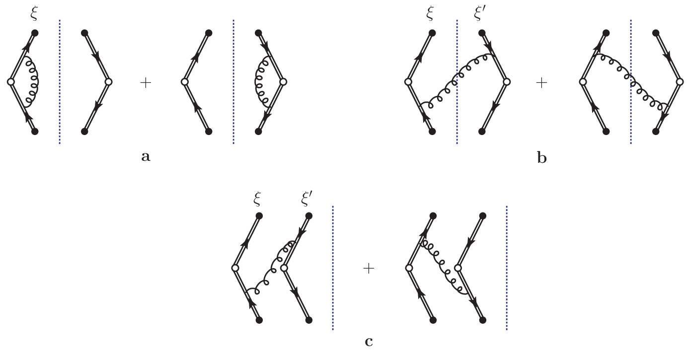

To regulate ultraviolet divergences, we work in dimensions, and to exhibit infrared divergences in individual graphs we use a small gluon mass . For the time being we omit the color matrices in the Feynman rules. One finds that each pair of graphs in figure 23 gives the same result, so that in the following we only list the expressions of the left-hand graphs and multiply by two.
Before renormalization, the vertex correction graphs in figure 23a give
| (182) |
where we recall that the vectors and have zero transverse momenta and satisfy , , , . For all poles in are on the same side of the real axis, so that this region gives a zero contribution to the integral over . For we close the integration contour in around the pole of the gluon propagator and obtain
| (183) |
As both poles in are on the same side of the real axis, one can deform the integration contour to and obtains
| (184) |
We see that both vectors and must be chosen away from the light cone, since taking even one of them lightlike gives an infinite result for . With the definition (180) for the rapidity of a spacelike vector, we have
| (185) |
We require a large rapidity difference, , i.e. . This is satisfied by the choice and made in section 3.2.2, but it also allows one of or to have central rapidity, as long as the rapidity of the other one is large (positive or negative). We can then approximate . The expression (184) is ultraviolet divergent, and using subtraction we obtain the renormalized result
| (186) |
For the graphs in figure 23b, which describe gluon emission into the final state, we have
| (187) |
Comparing with (183) we observe that at . For the integral over in (187) is ultraviolet finite and no subtraction is needed before we set . We thus obtain
| (188) |
where and is the Euler number.
The graphs in figure 23a and b give the full contribution for the vacuum matrix element defined in (177), which appears in single Drell-Yan production. Let us evaluate this contribution as a side result. The color factor for all graphs is in this case, so that we have with
| (189) |
for . Notice that the infrared divergences regulated by a gluon mass have cancelled in the sum over all graphs, as is required for a perturbative evaluation of . For the relation ensures that the condition does not receive radiative corrections, in agreement with the general result discussed below (177). This complete cancellation between real and virtual corrections plays a crucial role for collinear factorization, see section 3.5. The fact that the limit of (189) is infinite rather than zero is due to our use of modified minimal subtraction. For the ultraviolet divergences in and cancel each other (as do the finite parts of the graphs), so that there is no ultraviolet subtraction for their sum. At , however, does require ultraviolet subtraction since the first term is ultraviolet divergent whereas the second term is not.
Finally, the graphs in figure 23c give
| (190) |
For all poles in are on the same side of the real axis and give a zero net result, whereas for the integral over can be obtained from the residue of the gluon propagator. This gives the same expression as in the second step of (187). The graphs in figure 23c hence give the same result as those in figure 23b:
| (191) |
Note that the graphs in figure 23b and c only differ by the position of the final-state cut. The result (191) shows that this does not matter and provides a consistency check for the omission of explicit time ordering in (170). Namely, time ordering of the two fields and associated with the gluon propagator is required when the gluon does not cross the final-state cut. When it does cross the cut, no time ordering prescription arises, however, since the two fields then have a complete set of final states between them: .
The identity (191) also holds before setting and can then be used also at . This provides a simple explanation of the relation discussed above. Indeed, the equality is already evident from the starting expressions (182) and (190), which only differ by the sign of the eikonal propagator . This is a direct consequence of the Feynman rules in figures 16, since the upper eikonal lines to which the gluon couples in figures 23a and c only differ by the flow of color charge.
3.3.2 Soft factor associated with two-quark distributions
With these building blocks at hand we can construct the soft factor associated with two-parton distributions in the cross section formula (176). We first discuss the factor in some detail and give the results for and in the end.
The graphs contributing to are those in figure 25. In the graphs of figure 25a and b1 there is either no gluon coupling to the pair or no gluon coupling to the pair of eikonal lines, so that the lines have the same color coupling at the bottom and the top of the graph. The color factor for the vertex correction graphs 25a is , independent of the color flow along the eikonal lines and of the way in which their color indices are coupled. For figure 25b1 we have color factors
| (192) |
where the prefactors and come from the analog of the color decomposition (174) for . We note that these color factors are the same as for the ladder graphs we shall discuss in section 5.1.3.


By contrast, the graphs in figure 25b2 and c can change the color coupling of the eikonal lines. As an illustration, consider the first graph in figure 25b2 with the color indices at the bottom multiplied by octet matrices . The color structure is then
| (193) |
and we see that this graph contributes to both and . If the indices and are coupled to singlets, then the graph is proportional to and thus contributes to . For the first graph in figure 25c the color factors are analogous, with the difference that one has
| (194) |
instead of (193). Putting everything together and using the results of the previous section, we have
| (195) |
The terms come with an overall minus sign, because in graph 25c one of the eikonal lines coupled to a gluon has its color flow reversed compared with graph 23c, which reverses the sign in the eikonal propagator according to the Feynman rules in figure 16.
The matrix elements in (195) are such that we can replace and by their sum, which is infrared finite according to (189). Using we have
| (196) |
with a color factor
| (197) |
and linear combinations
| (198) |
Note that the dependence of has canceled in and .
At one-loop level the soft factor for two-quark distributions can thus be expressed in terms of its analog for single-parton distributions. This simplification will most likely no longer hold at higher orders in , since one then has graphs like in figure 26, where more than two eikonal lines are connected.

It is easy to see that the soft factor for quark-antiquark distributions is obtained from by replacing . This corresponds to the interchange of the labels and in the definitions of and (see (85) to (87)) and uses the result that the kernels and for gluons that cross or do not cross the final-state cut are identical.
The soft factor multiplying the interference distributions is obtained from the same graphs as those in figure 25, apart from changes in the color labels and in the color flow of the eikonal lines. Making the appropriate replacements of position arguments in we get
| (199) |
which can be rewritten as
| (200) |
3.4 Collins-Soper equation
As is well-known, cross sections with measured transverse momenta much smaller than the hardest scale in the process contain large logarithms in , which need to be summed to all orders in in order to have a perturbatively stable result. A powerful method to resum these Sudakov logarithms is due to Collins, Soper and Sterman (CSS) [118]. This method uses transverse-momentum-dependent factorization and is therefore, up to now, limited to the production of color singlet particles, such as a Drell-Yan lepton pair or a Higgs boson. In this section we show how this formalism extends to double Drell-Yan production, and we calculate the corresponding Sudakov factor to next-to-leading logarithmic accuracy.
We begin by a brief account of the CSS method for processes with a single hard scattering initiated by quark-antiquark annihilation. As we mentioned in section 3.2.3, the Wilson lines in the definition of transverse-momentum dependent parton distributions must be taken along a direction with a finite rapidity. Their dependence on this rapidity is governed by the Collins-Soper (CS) equation [48], whose solution resums Sudakov logarithms to all orders. By Lorentz invariance, the distributions depend on via the scalar parameter1212 12 To avoid the appearance of square roots, our definition (201) follows the convention of Ji et al. [51] and differs from the one of Collins and Soper [48], with .
| (201) |
As discussed earlier, we require to be spacelike (although the manipulations in the following would also work for timelike , which is the choice adopted in [51]). In terms of the rapidities of and of the proton, we have
| (202) |
for a right-moving proton, where is the proton mass. The approximations are valid for , which we have seen to be necessary in section 3.2.1. This implies .
Following the original paper [48] we work here with “unsubtracted parton distributions” in the parlance of [51, 119] and [50], i.e. with matrix elements of operators constructed from quark fields and Wilson lines along as in (162). Subtractions for the soft momentum region are not made in the parton distributions but in the soft factor that appears in the cross section (see [49]). The fields in the operator are renormalized, so that the distributions depend on an ultraviolet renormalization scale . Fourier transforming from transverse momentum to position space, we then have single-quark distributions . The dependence is given by a homogeneous renormalization group equation [48]
| (203) |
where can be identified with the anomalous dimension of the quark field in the axial gauge (where the Wilson lines reduce to unity). In a covariant gauge it corresponds to renormalization of the composite operator or , see (162).

In terms of graphs, the dependence of on arises from the propagators of eikonal lines and from their coupling to gluons, as is obvious from the Feynman rules in figure 16. A power counting analysis shows that dominant contributions to come from regions where the momentum flowing through eikonal lines is either hard or soft; contributions with collinear to the proton are power suppressed. The only important graphs where is a hard momentum have the form of a vertex correction shown in figure 27a (at higher orders this vertex graph becomes dressed with further gluon and quark lines). If the momentum flows through spectator partons (see figure 27b and c), the hard region is power suppressed and only the region of soft is important.
The contribution from the region of hard momenta reads
| (204) |
Since is hard, the kernel can be calculated perturbatively. is extracted from subgraphs whose external lines are the quark on the left of the final-state cut and the adjacent eikonal line, or the corresponding two lines on the right of the cut. As a result, is independent of the transverse distance between the two quark field operators. Furthermore, it depends only on the longitudinal quark momentum rather than on the proton momentum , so that the dependence on is via the combination . For dimensional reasons this parameter must be divided by , since is dominated by hard momenta and hence independent of nonperturbative scales. At leading order in , one obtains from the graph of figure 27a and the complex conjugate graph, with subtractions made for the region of soft . Using subtraction for the ultraviolet divergences, one finds [48, 119]
| (205) |
If the momentum carried by the eikonal lines and hence by the gluons they couple to is soft, we have graphs with soft gluons coupling to parton lines that move fast to the right. We can then use the same procedure as in section 3.2.2, i.e. approximate the gluon coupling to the right-moving particles and then use a Ward identity. The gluons then couple to eikonal lines with large positive rapidity, associated with a vector , with one eikonal line for each parton line attached to the collinear subgraph. This gives
| (206) |
where we used and where we have explicitly displayed the dependence of defined in (177) on the two vectors and . As shown in [50], one can take the limit of lightlike in (206) and thus has
| (207) |
with
| (208) |
Having taken the limit of infinite the dependence of on has disappeared as well, since by Lorentz invariance could only depend on . For large the kernel is dominated by nonperturbative dynamics, just as . For sufficiently small we can however use the perturbative expression of derived in the previous section. From (189) we readily obtain
| (209) |
verifying that at lowest order is independent of and .
An analysis of the ultraviolet divergences in and shows that they satisfy renormalization group equations [48]
| (210) |
so that the sum is independent of . At lowest order in this is readily verified from (205) and (209), which also give the leading term
| (211) |
of the anomalous dimension. The term is also known [118].
We are now ready to generalize the CS equation to (unsubtracted) two-quark distributions. The contribution from hard eikonal momenta is again given by vertex graphs as in figure 27a, with one graph for each of the four quark legs. This gives just the sum of kernels . As for the soft momentum region, the argument leading to (206) can be repeated. In section 3.2.2 we have seen that the Ward identity for soft gluons coupling to collinear lines in a two-parton distribution has a nontrivial color structure. We therefore now have a matrix equation in color space,
| (212) |
with a kernel
| (213) |
Analogous equations hold for quark-antiquark and for interference distributions, with kernels constructed from the appropriate soft factors . Note that the kernels are sensitive to the color charge of partons (i.e. to the difference between quarks and antiquarks) but not to their polarization. For this follows from the analogous property of , whereas for it follows from parity invariance applied to the relevant subgraph with one external quark and one eikonal line. Putting everything together, we can write the CS equation for a two-quark distribution into the form
| (214) |
with
| (215) |
According to (210) the dependence cancels between the kernels and in (214). The matrix is independent of as well. This can be traced back to the fact that the only ultraviolet divergent graphs for (and hence for ) have the form of a vertex correction as in figure 25a. As discussed in the previous section, these graphs only contribute to the color diagonal elements and and are the same in both cases, since they are insensitive to the color of the different eikonal lines.
Finally, the dependence of , etc. on the renormalization scale is given by
| (216) |
for both and . This is because ultraviolet renormalization in is performed for individual operators and .
3.4.1 General solution
Before solving (214) let us first consider the simpler equation
| (217) |
where we have abbreviated
| (218) |
We have included the argument of the running coupling in since this will be needed shortly. For the moment we do not assume that is given by a perturbative expansion. The solution of (217) can be obtained by adapting the well-known solution of the CS equation for single-parton distributions [48, 118, 120]. We have
| (219) |
where specifies the initial condition of evolution in . The scale should be chosen such that does not depend on widely disparate scales. If this is not possible because and widely differ in size, further steps may be required in order to resum all large logarithms. We note that since is independent (see below), the dependence of is given by the same renormalization group equation as in (216). The Sudakov exponent in (219) reads
| (220) |
with equal to or . It is well-known from the solution
| (221) |
of the CS equation (207) for single-quark distributions. We note that a more general set of solutions can be obtained by multiplying with a constant in the upper integration limit of (220); the initial condition in (219) then depends on that constant. One can easily restore the dependence of the expressions to follow, but for simplicity we limit ourselves to the choice here.
The integrand of (220) contains functions that depend on the ratio of two large scales. To make this dependence explicit, one uses the renormalization group equation (210) for and . Obviously, has the same dependence as , so that the dependence cancels between and in (217) and (220). Using (210) one can rewrite
| (222) |
Inserting this into (220) one can perform the integration over for the terms containing or and obtains
| (223) |
The term with in (223) gives rise to the leading double logarithm in , whereas the other terms give only single logarithms. Using (205) and (211) and neglecting the running of one has
| (224) |
at leading order in . A more precise expression is obtained by rewriting , where . After expanding in , the integral in (223) is straightforward to evaluate for the one-loop expression (205) of and the two-loop expression of (given e.g. in [118]).
The form (223) is valid even if cannot be evaluated perturbatively because one or both of and are large. If both distances are small, and thus is given by a power series in . An alternative form of the Sudakov exponent [118] is then obtained by rewriting (222) as
| (225) |
with
| (226) |
where we now distinguish between the explicit dependence of and the implicit dependence via the running coupling. One then obtains
| (227) |
where all perturbative functions are evaluated with at the same scale. With the one-loop expression of in (209) we have
| (228) |
A natural choice for the starting scale of evolution in is thus
| (229) |
with a constant of order 1. If one takes then vanishes.
It is now easy to write down the solution of the full CS equation (214) for a two-parton distribution. It is given by
| (230) |
with given by (223) for arbitrary values of and by (227) if both and are small. The logarithm in the second line has been chosen such that it coincides with the one that multiplies when one evaluates from (223). Other choices are possible and lead to different initial conditions and .
Unless all distances , and are small, the matrix cannot be calculated perturbatively and we cannot further simplify the exponentiated matrix in (230). Nevertheless, (230) contains some important information, since it gives the explicit form of the dependence on the large scales and . In particular, we see that to leading double logarithmic accuracy, where only squared logarithms of and are retained, the Sudakov factor for two-quark distributions is the same for and for and given by the product of the corresponding Sudakov factors for single-quark densities with momentum fractions and . At next-to-leading logarithmic accuracy, and mix under evolution in , with the amount of mixing depending on the transverse distances , and .
3.4.2 Small transverse distances
Let us now consider the situation when , and are all small enough to calculate in perturbation theory. The kernels in (214) are then given by (209) at leading order in , and the Sudakov exponent in the solution (230) of the CS equation can be evaluated from (227). It remains to investigate the matrix in (230), where we abbreviate
| (231) |
We treat the kernel for two-quark distributions in detail and discuss its analogs for quark-antiquark distributions and interference distributions later.
Using the definitions (213), (215) and our perturbative result (196) for , we readily find
| (232) |
with given in (197) and
| (233) |
in analogy to (198). Using the explicit form (209) or the renormalization group equation (210) for , we see that is independent, as we anticipated earlier. We must of course choose a scale in when using the one-loop result (209) for evaluating and , which gives rise to a residual scale dependence of order . The situation is the same as for a physical (and hence formally independent) quantity evaluated in fixed-order perturbation theory. An appropriate scale of in and will be constructed from and .
Let be the diagonal matrix with the eigenvalues of and let be the matrix whose columns are the corresponding eigenvectors, i.e.
| (234) |
One then has
| (235) |
The matrix (232) has eigenvalues
| (236) |
and a matrix of eigenvectors
| (237) |
so that
| (238) |
Let us see how this matrix behaves for
| (239) |
One can then Taylor expand the square root in (236) and obtains
| (240) |
if , whereas the role of and in (240) is interchanged if . In both cases one gets
| (241) |
where we have traded the color factor for
| (242) |
Since , the condition (239) holds in the large- limit. Inserting (241) into (230), we see that is then controlled by the initial condition because the admixture from is suppressed, although only by . Whether is dominated by or depends on whether the suppressed factor in the lower row of (241) or the exponential is smaller. In either case is parametrically smaller than . To which extent the large- limit gives a valid description of the physics for depends on the relative size of and , as well as the relative size of and . This can only be decided by a more detailed analysis, which we will not attempt here.
There is, however, a region of phase space where (239) holds beyond the large- limit. From its definition (233) we see that vanishes if . In the double-scattering process one has , so that the limit is relevant in the region where is much larger than . Taylor expansion then gives
| (243) |
This implies
| (244) |
for the factor in the off-diagonal elements of the matrix (241), whereas for the exponential factor we find
| (245) |
where we have chosen as in (229). We thus find that the octet admixture in the evolution of is power suppressed by , and that is power suppressed compared with by
| (246) |
In straightforward generalization of single Drell-Yan production [48, 50], an adequate choice of in the cross section for double hard scattering is . Together with this gives . Again, a more quantitative picture can only be obtained by a detailed analysis.
The preceding results all rely on the validity of perturbation theory for the soft CS kernel and thus require not only and but also to be perturbatively small. We cannot draw any strict conclusions about the case where and are small, whereas is in the nonperturbative region. However, we observe that the power suppression parameter becomes smaller rather than larger in this case. One may thus speculate that the general features of our analysis, namely the autonomous evolution of and the suppression of will continue in the nonperturbative regime.
We conclude this section by noting that the CS equation and its solution for quark-antiquark distributions is readily obtained from the previous results by replacing and that corresponding replacements are to be made for and . This follows from the corresponding property of the soft factor discussed at the end of section 3.3.2.
Interference distributions.
The Collins-Soper equation for interference distributions and has the same form as (214) with replaced by . The appropriate kernel in the perturbative regime follows from in (200) and reads
| (247) |
with and given in (233). This matrix has eigenvalues
| (248) |
and exponentiates to
| (249) |
For , i.e. if , we can Taylor expand the eigenvalues as
| (250) |
The result simplifies if we use the orthogonal matrix
| (251) |
that implements the basis transformation from to the combinations introduced in (117). We then have
| (252) |
Repeating the argument that led to (246) we obtain
| (253) |
with given in (245). Likewise, comparing (252) with (241) we find
| (254) |
For the sextet combination of is hence suppressed compared with the antitriplet one, which in its turn is small compared with the singlet combination .
We finally note that, in contrast to the case of , the limit just discussed does not give the same result as the large- limit. In the latter one finds
| (255) |
with relative corrections of order . This expansion is obviously not useful if one has . More generally, the large- limit for the evolution of will only be useful in kinematical regions where is small enough for .
3.5 Collinear factorization
The analysis in the previous sections was concerned with transverse-momentum dependent (TMD) factorization, i.e. with cross sections differential in transverse momenta that are small compared with the large scale. We now turn to collinear factorization, adequate for cross sections with integrated transverse momenta. We point out the main changes compared with TMD factorization but do not work out the formalism in detail.
As in previous sections, we first recapitulate the situation for single Drell-Yan production. The main changes compared with TMD factorization are as follows.
- •
We recall from section 3.2.2 that, after a complex contour deformation that avoids the Glauber region, the effect of soft gluon exchange is described by a soft factor . Integration of the cross section (178) over sets equal to zero in this factor. Because the cancellation between real and virtual graphs gives as discussed in section 3.3.1, there is no net effect of soft gluons in the integrated cross section.
With the elementary soft factor reduced to unity, subtractions of soft-gluon contributions as discussed in section 3.2.3 are not required, neither for the parton distributions nor for the hard-scattering subprocess.
- •
Setting in the quark and antiquark distributions , which is equivalent to integrating over , gives rise to short distance singularities in addition to those that are removed by defining the distributions with renormalized quarks fields and Wilson lines. The dependence on the ultraviolet subtraction scale is described by the well-known DGLAP evolution equations.
The rapidity divergences (from gluons with small and large ) that prevent us from taking lightlike Wilson lines in the definition of cancel between real and virtual corrections when [116]. Indeed, the relevant one-loop graphs are those in figure 27b and c (without the derivative ), and the approximation discussed in section 3.4 , which connects these graphs to the soft factor , is valid for any as long as is small.
Collinear parton distributions can hence be defined with lightlike Wilson lines and do not depend on a parameter . Correspondingly, the integrated cross section is free of Sudakov logarithms. In the operator definition of , the Wilson lines in and merge to a single Wilson line , given by
(256) The sections of the paths that go to infinity in and have cancelled, and a path of finite length between and remains.
- •
The hard-scattering subprocess now receives radiative corrections not only from virtual graphs but also from real ones, since emission of partons with large transverse momenta in the final state is permitted once we do not fix the transverse momentum of the Drell-Yan photon. As already mentioned, a subtraction for the soft-gluon region is not required in this case, in contrast to the situation for TMD factorization discussed in section 3.2.3. Subtractions are however needed for the regions where momenta are collinear to one of the partons entering the hard subprocess. These subtractions must be performed in a way that matches the ultraviolet subtractions in the parton densities. In particular, the dependence due to collinear subtractions in the hard subprocess has to cancel against the dependence of the parton distributions in the cross section.
Let us now investigate the situation for double Drell-Yan production, limiting ourselves to a one-loop analysis as we have done throughout the preceding sections. A key to understanding the role of soft gluons is to set in , which results from integrating the cross section (176) over . Our discussion in section 3.3.1 implies that for the graphs in figure 23. Together with the relation , this turns our general one-loop result (195) into
| (257) |
at . The one-loop contributions to cancel between the vertex corrections 25a and the real graphs 25b1, in full analogy with the case of discussed above. In and we have a cancellation between the real graphs 25b2 and the virtual graphs 25c.
We see from (257) that in the integrated cross section for double Drell-Yan production the contributions from color singlet and color octet distributions decouple from each other, and that they have a different behavior concerning soft gluon exchange. In the term with color singlet distributions we have a cancellation of soft gluon effects, in full analogy to single Drell-Yan production. Also, the graphs for the hard-scattering subprocess are exactly as in the single Drell-Yan process, with a cancellation of the soft-gluon region but with necessary subtractions for the regions of collinear parton momenta. From our above discussion it follows that collinear two-parton distributions can be defined with the same operators as their single-parton analogs, with lightlike Wilson lines and between quark and antiquark fields, and that their contribution to the integrated cross section is free of Sudakov logarithms. Like their single-parton counterparts, the distributions have ultraviolet divergences; the scale dependence that follows from their subtraction will be discussed in section 5.3.2.
The contribution of collinear color-octet distributions is quite different. Because real and virtual graphs have different color factors, soft gluon effects do not cancel between them, and their net effect is described by . As a consequence, the different factors in the cross section formula require soft subtractions, as they do in the case of measured transverse momenta. Since the color indices of and are not contracted, the two Wilson lines do not merge into a single one of finite length, and the same holds for their analogs with arguments and . The vector in the Wilson lines cannot be taken lightlike, so that collinear octet distributions will depend on a parameter . The resulting Collins-Soper equation gives rise to Sudakov logarithms, which suppress the color octet contribution to the integrated cross section. This important result was already obtained in [121], based on the observation that in the hard-scattering subprocesses there is no cancellation of the soft-gluon region. An adequate scale for the initial condition of the CS equation will in this case be a hadronic scale, inverse to the typical distance between the two scattering partons.
Let us finally take a look at the interference distributions . From (199) we find a soft factor
| (258) |
at . There is hence no cancellation of soft-gluon effects, so that a formulation of collinear factorization will in this case be similar to the one for the color octet distributions just discussed, with the additional complication of mixing between the color singlet and octet channels.
4 Some properties of two-quark and quark-antiquark distributions
4.1 Spin structure
Multiparton distributions have a nontrivial spin structure because the polarizations of different partons can be correlated among themselves, even in an unpolarized proton. In the following two sections we first investigate some general properties of spin correlations between two quarks and then show that they have observable consequences in multiple scattering cross sections. We will encounter several examples for parton spin correlations in section 5.2.2.
4.1.1 Spin decomposition
Let us first take a closer look at the spin dependence of the two-quark distributions introduced in (86), making use of rotation and parity invariance. We always assume that the hadron is unpolarized, i.e. that the matrix element (86) is averaged over the hadron spin. The simplest cases are the distributions
| (259) |
which are parity even, i.e. scalar functions. By contrast, the distributions and are parity odd, i.e. pseudoscalar functions. Their general form is
| (260) |
where , and are scalar functions with the same arguments as in (259). The scalar functions are in general neither even nor odd in or since their dependence on , and is not constrained by symmetry. Note that the three two-dimensional vectors , and are linearly dependent, so that the three cross products in (260) are linearly dependent as well. Expressing e.g. as a linear combination of and one obtains
| (261) |
and can thus write as times a single scalar function. However, that scalar function is singular when and become collinear, as is evident from the denominators in (261). To avoid such artificial singularities, one can use (260) if it is necessary to make the appearance of explicit.
Using that projects on quarks with definite helicity, one can readily identify the combinations of quark polarizations that are described by the above functions. In a schematic notation one has
| (262) |
where the superscript in denotes the quark helicity. The distribution thus describes the degree to which the two quark helicities are aligned rather than antialigned, whereas and describe the correlation between the helicity of one of the quarks and one of the cross products in (260).
To illustrate that spin correlations between two partons need not be small, let us consider the simple case of a symmetric three-quark wave function of the proton. Its spin-flavor part reads
| (263) |
where and respectively indicate that the quark spin is aligned and antialigned with the proton spin. As is well known, this wave function gives and for the longitudinal polarization of and quarks, which reproduces at least the trend of what is empirically found for the lowest moments of the polarized quark densities. For two-quark distributions one finds
| (264) |
and thus an appreciable correlation between the longitudinal polarizations of the quarks.
Of course, the study of a three-quark wave function tells us little about partons with or smaller, which are of particular relevance for LHC phenomenology. To the extent that they are known, polarized single-parton densities in this range are small compared with their unpolarized counterparts, which means that there is only a weak spin correlation between a small- quark and the proton as a whole. This is not too surprising, given that a small- quark and the proton are far apart in phase space. It does however not imply small spin correlations between two quarks that have small but comparable momentum fractions and are thus closer in phase space. How large such correlations are is an important open question.
The distributions defined with one or two tensor operators are associated with transverse quark polarization, since projects on quarks with a transverse spin vector . We now discuss their parametrization in terms of scalar or pseudoscalar functions. Let us begin with and , which transform like two-dimensional vectors. They can hence be written as a sum of three scalar functions that are respectively multiplied by , and . Only two of these functions are independent because of the linear dependence of the three vectors. A minimal parametrization is obtained by taking and
| (265) |
as basis vectors. This gives
| (266) |
where we have inserted the proton mass on the r.h.s. so that and have the same mass dimension as . Here and in the following we denote scalar functions by and pseudoscalar ones by . The latter can be represented in the same way as . If one wants to avoid pseudoscalar functions, one can replace the basis vector by
| (267) |
Since both and are orthogonal to , they must be proportional to each other, and explicitly one finds
| (268) |
If one inserts this into (266) then is multiplied by scalar functions, which are however singular when and become collinear. One could replace in (267) by another linear combination of and , but this would only move the singularities to a different part of phase space.
The distributions and transform like axial vectors, so that one has
| (269) |
A decomposition in terms of scalar functions can be obtained by replacing with . The tensor distribution can finally be written as
| (270) |
Notice that the four basis tensors in this decomposition are orthogonal to each other, i.e. with . Contracting (270) with the transverse polarization vectors of the quarks, we see in particular that goes with and thus describes the correlation between the two transverse quark spins.
In summary, we can represent the spin structure of by eight scalar and eight pseudoscalar functions for each combination of quark flavors. The pseudoscalar functions can be traded for scalar ones, which have however artificial singularities for particular values of the vectors , and .
If one integrates over transverse momenta to obtain collinear distributions, one finds
| (271) |
because one cannot construct a pseudoscalar function with only one vector . Likewise, the functions in (266), (269) and (270) integrate to zero, so that we are left with
| (272) | ||||||
The eight functions on the right-hand side now depend on , and and are obtained from their counterparts in (259), (266), (269) and (270) by integration over and .
The above decompositions are given for distributions in a right-moving proton. For a left-moving proton one has to change the sign of and hence of and of all pseudoscalar functions, see our remark below (100). Analogous decompositions can be written down for distributions , , that involve antiquarks, as well as for interference distributions and .
Symmetry properties
The terms appearing in the decompositions (259) to (272) are consistent with rotation and parity invariance. Let us now discuss their symmetry properties. Using that the operators in (80) satisfy one finds that the distributions are real valued,
| (273) |
For distributions that are purely defined in momentum or position space, see (9) and (12), this implies
| (274) |
These functions are in general not real-valued, nor are the scalar or pseudoscalar functions one can introduce to parameterize them in analogy to (259) to (270).
For the symmetry properties of parton distributions with respect to time reversal, the Wilson lines appearing in their definition are essential. As we argued in section 3.2.1, multiparton distributions involve the past pointing Wilson lines given in (156). Upon time reversal these turn into the future pointing Wilson lines in (160). A distribution is called even (odd) if it is even (odd) under time reversal without taking into account this change of Wilson lines. The time reversal invariance of strong interactions thus implies that odd distributions are only nonzero thanks to Wilson line effects; a prominent example from spin physics is the Sivers distribution function [122]. However, time reversal does force distributions to vanish if they are odd and have Wilson lines that are invariant under time reversal. This is the case for the Wilson lines along a finite lightlike path that appear in collinear single-parton densities and in the collinear two-parton distributions in the color singlet sector, as we discussed in section 3.5. By contrast, collinear color octet distributions , as well as interference distributions and , have Wilson lines that do change under time reversal.
After these preliminaries we can now investigate the time reversal properties of two-quark distributions. We find
| (275) |
with sign factors and , where the superscripts indicate the type of Wilson line in the matrix element defining the distributions. The relations (273) to (275) also hold for the distributions , , with antiquarks and for the interference distributions , .
Since the scalar functions parameterizing are in general neither even nor odd in , they are not even or odd either. The scalar functions that parameterize the collinear distributions in (272) are however even in . As a consequence, and are odd and all other distributions in (272) are even. For the color singlet sector this implies
| (276) |
whereas the corresponding color-octet distributions and can be nonzero due to the Wilson lines appearing in their definitions. Analogous statements hold for the corresponding distributions with one or two antiquarks. Collinear interference distributions and are not restricted by time reversal invariance.
4.1.2 Spin effects in gauge boson pair production
In this section we show that the quark spin correlations discussed in the previous section have observable consequences in multiparton interactions. As we did earlier in this paper, we consider the production of a pair of gauge bosons , or . We include the decay of each boson into a lepton pair, which carries information on the spin state of the gauge boson. While these processes have a rather small cross section, they may be suited for experimental studies due to their clean final-state signature. We do not present a full analysis here, but highlight the effects of selected parton spin correlations.
For simplicity we limit our attention to those distributions that do not involve explicit vectors or on the r.h.s. of the decompositions in the previous section, i.e. to , and the term in . For definiteness we analyze the graph of figure 6a, with two quarks emitted from the right-moving proton and two antiquarks from the left-moving one. We approximate the transverse momenta of the bosons by zero when calculating their production and decay, as deviations from this limit are suppressed by powers of . The partonic cross section for the production of a lepton pair can be written as the product of a production tensor of the boson and a tensor for its decay,
| (277) |
where is associated with the boson in the amplitude and with the one in the complex conjugate amplitude. For unpolarized or longitudinally polarized quarks one easily finds
| (278) |
with coefficients and depending on kinematic variables and the vector and axial-vector couplings of the gauge boson to the quark . In the case of a photon one has . The transverse tensors and have as nonzero components and . From (278) it follows that the overall cross section depends on the combinations
| and | (279) |
of multiparton distributions. The contraction of and with the vector boson decay matrices results in different angular distributions of the leptons. If one integrates over their angles then only the contribution from remains. We thus find that nonzero values of and modify both the total rate and the lepton angular distribution compared with the contribution from the unpolarized term .
We now turn to transverse quark polarization. In this case the production tensor from each hard scattering depends also on the transverse indices associated with the quark polarization. We recall that the quark field bilinears are chiral odd, so that in the helicity basis they correspond to quarks or antiquarks with opposite helicities in the scattering amplitude and its conjugate. As a result transverse quark polarization does not contribute to the production of a boson. Keeping only the term in the decomposition (270) of and the corresponding term in the decomposition of , one finds for the neutral bosons or
| (280) |
where the polarization indices belong to the boson with momentum and the indices to the boson with momentum . We observe that the polarization indices of the two bosons are entangled in (280). Contracting with the well-known boson decay matrices, one obtains an azimuthal dependence like , where is the relative azimuthal angle between the two leptons (as opposed to the antileptons).1313 13 Since we are working in the approximation , the azimuthal angles for the leptons of both boson decays are naturally defined w.r.t. the axis in the center-of-mass. We thus obtain the important result that a correlation between transverse quark and antiquark spins, as expressed by the distribution in (270), leads to a correlation between the decay planes of the two produced bosons.
It is instructive to rewrite the production tensors in terms of boson polarization vectors and , which respectively correspond to angular momentum or along the axis. One finds
| (281) |
and
| (282) |
We can easily understand why each boson is transversely polarized. Recall that a massless quark and antiquark can only annihilate into a vector boson if their helicities are coupled to . Since we neglect the transverse momentum of the bosons, their angular momentum along must also be . The tensors and in (281) correspond to the same boson polarization in amplitude and conjugate amplitude and thus do not give rise to an azimuthal dependence in the leptonic decays, but they do give different distributions in the polar angles of the leptons, or equivalently in their rapidities. By contrast, (282) involves the interference between and for each of the bosons, which readily translates into the dependence already mentioned.
It is natural to expect that spin correlations between partons also lead to angular correlations in the final state for other double-scattering processes, such as the production of two dijets. In this case two-parton distributions involving linear gluon polarization can contribute as well. We note that in the analysis of [9] uncorrelated dijet planes were taken as a characteristic feature of the double-scattering mechanism. This is only adequate if parton spin correlations in the proton are negligible.

Returning to four-lepton production, let us compare our results for double hard scattering with the contribution from a single annihilation, remaining in kinematics where and can be neglected compared with . The corresponding Feynman graphs involve either quark exchange in the or channel, or an intermediate boson in the channel in case one or both final-state bosons are charged, see figure 28a and b. In addition, the four-lepton final state can be produced by graphs as in figure 28c, where only one lepton pair comes from the decay of a vector boson. Such graphs were recently discussed and termed “single-resonance graphs” in [13]. They should be taken into account unless each lepton pair has an invariant mass inside the or mass peaks.
The dependence of the single-scattering cross section on the azimuthal angle between the leptons can be deduced from symmetry arguments since we set and to zero in the parton-level process. Let us assume that the initial pair has total angular momentum along the axis. This must then hold for both the scattering amplitude and its conjugate, since a single quark or antiquark in an unpolarized proton is unpolarized. One of the lepton pairs originates from the decay of a gauge boson and is thus in a partial wave with . The possible combinations of for the two lepton pairs are thus , , and , where the first and last possibilities are only possible for single-resonance graphs. In the cross section this gives a independent term and a modulation with from all graphs, as well as modulations with and from single-resonance graphs. The same angular terms are obtained when the initial pair has , whereas the configuration where the pair has decouples in the hard-scattering graphs of figure 28. In summary, the modulation we found in the double-scattering mechanism competes with single-scattering contributions involving single-resonance graphs.1414 14 This was not realized in [47], where single-resonance graphs were not taken into account. One may hope that the two sources of dependence can be separated by a more detailed analysis — making for instance use of the fact that the single-resonance graphs also give a term — but this issue must be left to a dedicated study.
4.2 Mellin moments and lattice calculations
If one takes Mellin moments in and of the color singlet distributions , then the light-cone operators in their definition turn into local operators. The corresponding moments of single-parton densities can be calculated in lattice QCD, and we will now investigate to which extent the same can be done for two-parton distributions. From our discussion in section 3.5 it follows that the Mellin moments of color octet distributions do not involve local operators because of their Wilson line structure. We therefore limit ourselves to the color singlet sector.
Using the relation (88) and its analogs for and , one obtains double Mellin moments
| (283) |
with and . For each label the moments and the corresponding operator on the r.h.s. carry an additional transverse Lorentz index not displayed in (283). On the r.h.s. we have the twist-two quark operators familiar from the operator product expansion,
| (284) |
where is the antisymmetrized covariant derivative. , and respectively denotes symmetrization, antisymmetrization and subtraction of traces in the indicated indices. It is understood that the composite operators and in (283) are each renormalized in a standard manner, e.g. in the scheme. As long as they are taken at a finite spacelike distance , no further ultraviolet divergences appear. The operators and mix of course with their gluon counterparts and under renormalization. We shall return to the renormalization of collinear multiparton distributions in section 5.3.2.
Let us rewrite the r.h.s. of (283) in a manifestly covariant form. We first introduce the covariant decomposition
| (285) |
where the ellipsis represents terms with uncontracted vectors and terms involving the metric tensor . The reduced matrix element can only depend on the invariants and . We then choose a frame where and , so that and . This allows us to write (283) in the desired form
| (286) |
A corresponding representation is readily obtained for . For one or two polarization labels the analogs of (285) involve the tensor structures in the decomposition (272) of the two-quark distributions.
The matrix element in (285) and its counterparts with polarized quarks can be evaluated on a lattice in Euclidean spacetime if one chooses . This is rather similar to lattice studies of transverse-momentum dependent single-quark distributions [123, 124], with the main difference that the operators taken at different spacetime points are single quark fields in that case, whereas they are gauge invariant bilinear operators here. The restriction entails
| (287) |
where and denote the spacelike three-vectors. Thus, the integral over all at fixed on the r.h.s. of (286) can unfortunately not be evaluated from results on a discrete Euclidean lattice, where the maximal momentum is fixed by the lattice spacing. This is completely analogous to the single-quark case, as discussed in [124]. Despite this limitation of principle, we hope that lattice data in a certain range of and will in the future provide genuinely nonperturbative information about the behavior of multi-parton distributions.
We note that a lattice calculation has been reported in [125] for the correlation function of two vector currents at equal time in a proton at rest. This corresponds to setting and in (285). The reduced matrix element at is directly related to an integral of the two-quark correlation function defined in (75). The relative plus-momentum is integrated over in that case, rather than being set to zero as required for the distributions that appear in double hard-scattering cross sections.
4.3 Relation with generalized parton distributions
In section 2.1.5 we derived an approximate relation between multi- and single-parton distributions in a model theory with scalar partons. We now extend this relation to distributions for two quarks or antiquarks, taking into account the different combinations of fermion number and color. For the time being we neglect aspects related to the proton spin, which will be discussed in section 4.3.1. The distributions we will deal with are
| (288) |
The general result (69) for scalar partons readily carries over to the two-quark distributions :
| (289) |
where the impact parameter dependent single-quark distributions are defined in analogy to the scalar case in (64) and (65). Setting in (289), one obtains collinear distributions on both sides and has the probability interpretation represented in figure 4. As a counterpart to (72) one can transform the relation (289) into transverse-momentum space, where it reads
| (290) |
with distributions defined in analogy to (66). Integrating over we obtain the relation recently given in [59]. Relations analogous to (289) and (290) are obtained for by replacing the label with on both sides.
To reduce to single-particle distributions we could repeat our earlier derivation that started with (59). We find it more convenient to work in the transverse-momentum rather than impact parameter representation. We insert a complete set of intermediate states between the color singlet operators and and assume that single-proton intermediate states dominate. We then have
| (291) |
After an appropriate shift of the position arguments in the bilinear field operators and a change of integration variables from to , and this gives
| (292) |
The integrations over and fix the momentum of the intermediate state. In particular, its plus-momentum is , which reflects that the operator describes the emission of a quark with plus-momentum and the reabsorption of a quark with plus-momentum . The matrix elements in the approximation (292) are thus given by generalized parton distributions (GPDs), which play a prominent role in the description of hard exclusive processes, see [126, 127, 128] and the reviews [129, 130, 131]. To evaluate the unapproximated form in (291) one would need the corresponding matrix elements for all transitions . This is obviously impractical, although for selected transitions to single baryons, e.g. for , some information can be obtained [129, 131]. GPDs are defined by
| (293) |
where and is one of the matrices in (81). The parameter
| (294) |
is often called skewness. One finds that is the average transverse momentum of the two quark legs and their average plus-momentum divided by the average plus-momentum of the proton states. For ease of notation we do not indicate the polarization states of the protons, which are in general different. A parameterization of the matrix elements (293) for spin hadrons in terms of scalar functions can be found in [132]. Invariance under the transverse boost specified by gives the relation with . Abbreviating
| (295) |
we can thus rewrite the relation (292) as
| (296) |
where and
| (297) |
In complete analogy one derives
| (298) |
where the generalized parton distributions for antiquarks are defined by replacing with in (293). One finds
| (299) |
with the same sign factors and that appeared in (88). We also note that generalized parton distributions with positive and negative skewness parameter are easily related to each other by taking the complex conjugate of (293).
For the distributions and we obtain
| (300) |
where we have again but now
| (301) |
In this case we have , which describes the emission of a quark-antiquark pair. Again, this could be anticipated from figure 5 since now the parton lines combined to color singlets are and , with each pair being on the same side of the final-state cut in the double parton distribution.
An important difference between the approximations for , , and the one for given in (289) is that the generalized distributions on the r.h.s. of (296), (298) and (300) do not reduce to collinear functions if we integrate over and , because these momenta appear in their fourth arguments.
The preceding derivations can easily be extended to distributions describing interference between different quark flavors. The distributions corresponding to figure 7 are defined with bilinear operators or . For a proton target, the ground state in the sum over intermediate states inserted between the two operators is then a neutron. Isospin symmetry relates the resulting matrix elements to matrix elements in the proton: . Under the assumption of flavor symmetry one can derive similar relations for distributions involving strange quarks [129, 131].
Although the relation between multiparton distributions and GPDs is an approximation whose accuracy is not easy to estimate (and although our current knowledge of GPDs is far less advanced than that of ordinary parton densities) this relation provides opportunities to obtain information about multiple interactions that is hard to get by other means. One example are the different interference distributions discussed above, which are so far entirely unknown. Perhaps even more important is that GPDs give rather direct information about the distribution of single partons in the impact parameter , which is Fourier conjugate to a transverse momentum transfer that can be measured in physical processes. This is in stark contrast to the interparton distance in two-parton distributions, which appears as an integration variable in cross section formulae like (91) and is not directly related to observable kinematic quantities. We already mentioned in section 2.6 that studies of GPDs give evidence for a correlation between the longitudinal momentum and the impact parameter of partons in the proton. For values of the momentum fraction where such a correlation is strong, it is hardly plausible that there should be no correlation between and in two-parton distributions, even if there were important corrections to approximations like (289).
4.3.1 Spin correlations
We now take a closer look at the role of the proton spin in the approximate relation between double and single parton distributions, which we have glossed over up to now. For our purpose, a suitable choice to describe the spin state of a proton is the light-cone helicity , which is equal to the usual helicity in a frame where the proton plus-momentum tends to infinity (see e.g. [133] or (130, section 3.5.1)). We denote the corresponding momentum eigenstates by .
When inserting intermediate proton states between the two color singlet operators in a two-parton distribution for an unpolarized proton, we schematically have
| (302) |
or an analogous relation with states of definite transverse position. The sum over states on the r.h.s. thus includes single-parton matrix elements where the proton helicity differs in the bra and the ket state. Corresponding sums over polarization states should hence be inserted in the relations (289), (296), (298) and (300).
To discuss the implications of this observation, let us focus on the collinear distribution . At the level of matrix elements we have a relation
| (303) |
where the superscripts and of denote the proton helicities as in (302) and an average over proton helicities is understood in . A standard decomposition of the spin dependence of generalized parton distributions involves two distributions and for unpolarized quarks and two distributions and for longitudinally polarized quarks. The distribution does not contribute in the case of zero skewness we are dealing with here. Using the conventions and the matrix elements for definite proton light-cone helicity in eq. (54) of [130], we have
| (304) | ||||||
| and | ||||||
| (305) | ||||||
where is the proton mass and , and are the usual GPDs defined in [130]. and are the respective generalizations of the unpolarized and longitudinally polarized quark densities and . Changing the basis of the proton spin states, one can see that is related to unpolarized quarks in a transversely polarized proton [65]. Inserting (304) into (303), we get
| (306) |
The term with corresponds to the simplest approximation of the two-parton distribution as a product of single-parton distributions, whereas the one with appears in addition. describes a correlation between the position of a single quark and the proton spin, and (306) shows how such a correlation may lead to a correlation between two quarks in an unpolarized proton. It is difficult to say whether this correction term alone already provides an improved approximation of , but one may take it as an indicator for the possible departure from a simple factorized ansatz that neglects all correlations. In cases where the correction from is large, it is plausible to expect that the factorized ansatz involving only will fail.
Applying the same method to the distribution , we obtain from (305)
| (307) |
Again one should be cautious regarding the validity of this approximation. For the region of small but similar and we already argued in section 4.1.1 that one may well have sizeable correlations between the longitudinal polarization of two quarks, even if there is little correlation between the longitudinal polarizations of one quark and the proton as a whole. Conversely, in kinematics where the product of quark-proton spin correlations in (307) is sizeable it seems natural to assume that quark-quark spin correlations are sizeable as well.
5 Perturbatively large transverse momentum
So far we have treated multiple interactions as a two-scale problem, in which the virtualities define a large scale whereas the transverse momenta , and the scale of nonperturbative interactions are treated as small. We now make a distinction between the different scales previously treated as small, requiring to be large compared with the hadronic scale . We thus have a three-scale problem characterized by the hierarchy
| (308) |
Large implies that at least some of the transverse parton momenta and must be large. The occurrence of partons with large transverse momentum can be thought of as resulting from the perturbative splitting of partons with low , which leads to a factorization formula for transverse-momentum dependent parton distributions in terms of a hard-scattering kernel and collinear distributions. This significantly adds predictive power since collinear distributions depend on fewer variables than dependent ones.
Example graphs for the case of a single-quark distribution are shown in figure 29. The description based on such graphs was extensively used for spin effects and azimuthal correlations in Drell-Yan production [134, 135, 136] and semi-inclusive DIS in [136, 137, 117], building on the seminal work in [48, 118].

This description carries over to the case of two-parton distributions and is discussed in section 5.1. In the subsequent sections we investigate a competing mechanism for the generation of high transverse momentum, in which the two partons with momentum fractions and originate from the perturbative splitting of a single parton. We will see that this mechanism has profound consequences for the theoretical description of multiple interactions.
5.1 Ladder graphs at large

The single and double ladder graphs in figure 30 are natural generalizations of the ladder graph for a single parton density in figure 29a. In the following we concentrate on these ladder graphs, bearing in mind that in a covariant gauge there are further graphs with eikonal lines as in figure 29b. Those do not change the conclusions we obtain for the ladder graphs. Indeed, they are absent in the axial gauge , where the Wilson lines in the definition of parton distributions reduce to unity (apart from pieces at infinity, as discussed at the end of section 3.2.1).
When interpreting the graphs in figures 29 and 30 it is important to bear in mind that they represent a separation of dynamics at different scales, with lines attached to the lower blob having virtualities of order , whereas propagators in the upper part of the graphs are for virtualities of the order of the large transverse momentum . An important feature of figure 30 is that no hard gluons are exchanged between the parton lines that have different momentum fractions and at the top of the graphs. The requirement that both and have small virtualities forces to be of order , which translates into interparton distances of hadronic size in the Fourier transformed distributions .
5.1.1 Power behavior
Let us first investigate the general power behavior associated with ladder graphs. In the following we refer to as the hard scale (compared with ), keeping in mind that is still much smaller than .
We proceed in a similar way as in section 2.4. In particular, we use the modified parton correlation functions , which contain a factor for each quark or antiquark of momentum and in which pairs of quark fields are contracted with a Dirac matrix from (81). For the transition from to partons in the channel, we correspondingly use hard-scattering coefficients that include a factor for each incoming quark or antiquark and a factor for each outgoing one. Spinor indices in are contracted with an appropriate matrix , , for outgoing lines and with , , for incoming ones. is invariant under a boost along and thus can only depend on the scale but not on (cf. the corresponding argument for in section 2.4). One thus obtains
| (309) |
as one can easily check for the example graphs below. Note that compared with the hard-scattering amplitudes in (127) we now have instead of because includes the propagators of the outgoing partons, as is appropriate for the calculation of parton distributions.
The power behavior for the single-ladder graph in figure 30a can be obtained from
| (310) |
The factor and the integrations over minus-momenta come from the definition of , whereas compensates the corresponding factors in and . It is understood that includes a function for each parton line going across the final-state cut. This does not affect the power counting, since one could first consider the hard-scattering amplitude without cut and then take the appropriate discontinuity in the channel. The momenta and attach to the parton distribution at the bottom of the graph and hence have virtualities of order , whereas emerges from the hard scattering and hence has virtuality of order . As a result, the momentum components and are small and can be neglected in the hard-scattering kernel . We used this when rearranging the order of integrations in the second step. By contrast, the large components and are to be kept in . For the power behavior we obtain
| (311) |
with (126) and (309). We recognize the behavior that is characteristic of the splitting of one parton (the incoming quark) into two partons (the outgoing quark and the gluon). The power behavior for the double-ladder graph in figure 30b is obtained by the same type of analysis:
| (312) |
If all transverse momenta are small, the distribution scales of course like .
Let us now see how the power behavior of the two-parton distributions translates into the power behavior of the cross section
| (313) |
where we have omitted numerical factors as well as labels for parton species, spin and color. We have multiplied the cross section with for convenience, since this gives factors of order on the r.h.s.
To have both large and requires at lowest order in either a single-ladder graph in the distribution for each colliding proton, or a double-ladder graph in one of the distributions with no hard gluons in the other, as shown in figure 31. In both cases one has for the product of distributions, and the integration volume is of order since and thus are restricted to be of size . Similarly, one finds in both cases, so that the overall power behavior is
| (314) |
By similar arguments one finds that the power behavior remains the same at higher order in , when one can have more than two ladders in the graphs for the cross section. Any decrease by a factor in the product is compensated by an increase from to in the integration volume over the transverse parton momenta or .

5.1.2 Factorization formulae
Let us now investigate the structure of the factorization formulae for ladder graphs. Still omitting spin and color indices for the moment, we write our result (310) as
| (315) |
The lower limit on the integration reflects that the gluon with momentum crosses the final-state cut and hence cannot have negative plus-momentum. Up to a numerical factor, the second expression in square brackets is just the transverse-momentum dependent double-parton distribution with . The first factor in square brackets is invariant under boosts along and can thus only depend on and . We can write it as a numerical factor times , where is dimensionless. If is a scalar it depends on only via and only because there are other dimensionful variables and , which we have not displayed for ease of writing. For certain parton polarizations, is a tensor with transverse indices and can hence depend on the components of , as discussed below.
We can finally Fourier transform (315) from to and then have
| (316) |
where the factor has been chosen for convenience. Inserting this and its analog for in the cross section formula (35), we have
| (317) |
where we have used the function constraints in (35) to eliminate and . We can now approximate and , after which the integrations over and only concern the double-parton distributions, which are then integrated over both transverse-momentum arguments. The result is
| (318) |
Only collinear two-parton distributions appear on the r.h.s., so that the relation (316) is only needed in the form
| (319) |
Repeating the preceding arguments for the double-ladder graph, one obtains
| (320) |
from the result (312) and
| (321) |
for the contribution of figure 31b to the cross section, where again only collinear two-parton distributions appear.
The analog of (319) for single-parton distribution reads
| (322) |
At order the kernel is just the usual DGLAP splitting function, up to terms proportional to which will be discussed shortly. To see this, let us consider the integrated parton density defined with a naive cutoff,
| (323) |
Using that the transverse-momentum dependent density depends only on the square of we then have
| (324) |
and comparing with the DGLAP equation for the l.h.s. we can identify the kernel in (322) as the familiar splitting function.
The preceding argument is oversimplified in two respects. Firstly, the calculation of for large only involves real graphs like those in figure 29 at leading order in , because to obtain a parton with large one needs a recoiling parton in the final state. (Higher-order graphs can include virtual loops, so that our argument cannot be applied any more.) By contrast, the evolution equation for the collinear parton density , which is integrated over all , involves both real and virtual graphs at order . The latter give contributions proportional to to the DGLAP splitting kernels, which are absent from in (322). Secondly, the distribution must be defined with non-lightlike Wilson lines as discussed in section 3, which leads to a dependence on the parameter defined in (201). Since the collinear distribution has no such dependence, it is the kernel in (322) that must depend on . The explicit calculation in [117] shows that the dependence of comes with a factor , which in the light of our discussion in section 3.2.3 is plausible if one observes that the point in (322) corresponds to infinite negative gluon rapidity in figure 29.
Let us mention that there is an analog of (322) for the distribution at small transverse distance . The corresponding hard-scattering kernel differs again from by terms proportional to . This is because is given by an integral over all , so that already at order virtual graphs appear in addition to real ones.
We now turn our attention to the role of color in two-parton distributions at high transverse momentum, which we have glossed over so far. Since the graphs we are discussing do not connect parton lines with different momentum fractions and , the color coupling of the distributions on the left and on the right of the factorization formulae (319) and (320) are the same. For distributions in the color singlet channel, the kernels in (319) and (320) coincide with the one in (322) at least at leading order in , since the relevant hard-scattering graphs to be calculated are identical. The leading-order kernels for the color octet distributions differ by an overall color factor from those for , which is the subject of the next section. Note that, unlike their color singlet analogs, the collinear color octet distributions appearing on the r.h.s. of (319) and (320) depend on as discussed in section 3.5. Given our discussion of the cancellation or non-cancellation of soft contributions between real and virtual graphs in section 3.5, we expect that the kernels for the position space distributions and at small will differ by more than an overall color factor already at leading order. A systematic investigation of this is left to future work.
The power counting in section 5.1.1 and the discussion in the present section do not depend on whether the parton lines in the ladder graphs are quarks or gluons. As is well-known for single parton distributions, a quark with high transverse momentum can originate from a gluon with low transverse momentum and vice versa. The corresponding elementary ladder graphs are shown in figure 32 below.
We now discuss the spin structure of the ladder graphs. As we have seen in sections 2.2.1 and 2.2.2, there are three polarization combinations for each quark or gluon in a two-parton distribution, which we can choose as unpolarized (), longitudinally polarized and transversely or linearly polarized. The possible transitions between these combinations in the factorization formulae (319) and (320) are restricted by symmetries. Transverse quark polarization is described by a chiral-odd operator and the chirality of light quarks is conserved in hard-scattering subprocesses, so that the only transitions for transversely polarized quarks are of the form . In the longitudinally polarized sector one has all possible transitions between and on the left and on the right of (319) and (320), with transitions to other polarizations being forbidden by parity invariance. Likewise, one has all possible transitions between unpolarized quarks and gluons. In addition, ladder graphs allow the transitions and from unpolarized collinear distributions to linearly polarized gluons at high , as has been observed in the study of single Higgs production in [83, 84]. Since corresponds to a helicity difference of two units between the gluon on the left and the gluon the right of the final-state cut, there is no collinear distribution for a single linearly polarized gluon in a proton, so that transitions and played no role in [83, 84]. However, one finds that the corresponding hard-scattering kernels are nonzero and hence allow these transitions for two-parton distributions. One thus has all possible transitions between and .
For distributions that involve polarizations or the kernels in (319) and (320) are tensors with transverse Lorentz indices, constructed from and from the large transverse momentum or in the ladder. Explicit calculation at order shows that the kernel for the transition from to (with arbitrary ) is proportional to . As a result, ladder graphs do not generate the distributions and in the decomposition (270) of , given that they come with tensors that are absent in the collinear distributions according to (272). This adds to the predictive power of the perturbative mechanism at large transverse momenta. For transitions involving linear gluon polarization we find kernels
| (325) |
where the transition from to is described by , the transition from to by etc., and where is or . The second tensor in (325) is symmetric and traceless and describes two units of orbital angular momentum, which compensates the mismatch of helicities in the transitions , , and . For later use we note that terms involving this tensor vanish by rotation invariance when (316) or (320) is integrated over and .
The representation of the cross section derived in this section is based on a two-step procedure. In the first step we have used factorization to separate the annihilation processes into vector bosons with mass or virtuality of order from transverse-momentum dependent two-parton distributions, in which the largest scale is . In a second step, we have used factorization to compute these distributions in terms of hard-scattering processes at scale and distributions that reflect physics at a hadronic scale , where it turned out that in the cross section we only need the latter distributions integrated over and .
An alternative procedure is to first use factorization to represent the graphs in figure 31 as the product of collinear two-parton distributions and inclusive hard-scattering processes , where at lowest order in the unobserved system consists of just one gluon. In a second step one can then simplify the corresponding hard-scattering kernels by taking the limit we are interested in. The relation between these two procedures has been studied in detail for single Drell-Yan production or for semi-inclusive deep inelastic scattering in [117] and [134, 135, 136, 137]. An important property of the procedure using transverse-momentum dependent distributions in a first step is that it permits the resummation of Sudakov logarithms with the method of Collins, Soper and Sterman [118].
5.1.3 Color factors and quark-gluon transitions

Let us now compute the color factors for the transitions from collinear to transverse-momentum dependent two-parton distributions, restricting ourselves to the leading order in . For this it is sufficient to consider ladder graphs for the hard scattering, because graphs with eikonal lines as in figure 29b can be eliminated by choosing the gauge . Multiplying the color structure of the ladder graphs in figure 32 with the appropriate color matrix for the incoming partons, one obtains the following color transitions:
| (326) |
Reversing the fermion lines in the ladder graphs changes the order of multiplication for the matrices on the l.h.s. of the above relations. This leads to a change of sign on the r.h.s. for the transitions and , whereas transitions between and or between singlets are unchanged. This implies that the difference of distributions for and does not mix with gluons in the singlet or the symmetric octet channel but does mix with gluons coupled to an antisymmetric octet.
In the cases where there is mixing, the relation (319) for a double-parton distribution at large becomes a matrix equation, which can be written as
| (327) |
where the arguments of and are as in (319). For polarizations and the distributions and kernels carry tensor indices, which were discussed in the previous section and will be omitted here. The matrix structure in (327) can be generalized to the relation (320) for double-ladder graphs, but the resulting expressions are rather cluttered with indices and will not be given here.
In the color singlet sector one has
| (328) |
where is the number of quark flavors and where the second parton may be an unpolarized or polarized quark, antiquark or gluon.1515 15 We note that in [47] the possibility of transitions between and was overlooked, and only the mixing between and was considered. To obtain the color factors for the off-diagonal elements one must take into account the prefactors in the definitions (103), (2.3.2) and (123). In the upper left submatrix of we recognize the structure of the mixing matrix in the usual DGLAP equations. Mixing in the symmetric octet sector involves the vectors
| (329) |
If indicates a gluon, one should replace by and by . The splitting matrices now read
| (330) | ||||
| and | ||||
| (331) | ||||
There is no mixing for the combinations , nor for the difference of distributions for two quark flavors, nor for matrix elements where the quark flavors differ on the two sides of the final-state cut as in figure 7. In these cases the behavior at large is described by (319) with replaced by for color singlet and by for color octet combinations.
Experience with the usual parton densities tells us that gluons quickly dominate over sea quarks as one goes to momentum fractions below (except possibly if one considers very low factorization scales). One therefore expects that for typical values of and at LHC, two-parton distributions at high transverse momentum are dominated by those combinations that can originate from gluons in (327).
Comparing (328) with (330) and (331) we find that the color factors are always smaller in the octet channels than in the singlet channel, with the biggest suppression occurring for . In the large- limit the singlet matrix has one eigenvalue and two eigenvalues with color factors for the submatrix in the sector. Both and have the same two eigenvalues, but with color factors instead of , and another eigenvalue of order . One can hence expect a dominance of color singlet distributions for sufficiently large transverse momentum, which would significantly simplify the theoretical description and the phenomenology of multiple interactions. How strong the suppression of color octet channels is in given kinematics should, however, be studied quantitatively before drawing strong conclusions.
We have also calculated the color factors for higher color representations of gluon distributions, restricting ourselves to as we did in (121). Mixing with quark distributions is of course not possible in this case. We find that the color factors for decuplet and antidecuplet distributions are zero, so that ladder graphs do not admit these color combinations, at least not at leading order in . For the representation we obtain
| (332) |
where or . The color factor is equal to and thus smaller in magnitude than the factors or we have in the singlet and octet sectors, respectively.
The color factors we have obtained agree with those given in [138], provided that one restores a missing factor in the expression of in eq. (54b) of that paper.1616 16 The projector in [138] appears only for with [139]. Our color factors for transitions in the gluon sector are also in agreement with eq. (A.6) in [140].
The splitting matrices for longitudinally polarized quarks and gluons in (327) are obtained from the upper left submatrices for unpolarized quarks and gluons in (328) to (331) by changing the kernels but keeping the color factors. Likewise, the splitting kernel for transverse quark polarization comes with the same color factors as . In both cases, it is again the color singlet sector that has the largest color factors and will therefore be enhanced at high transverse parton momentum.
Let us finally consider ladder graphs for the quark-antiquark interference distributions represented in figure 5c. The color independent part of the splitting kernel is different for distributions and because of their different spin structure (in one case a gluon is exchanged between a quark and an antiquark line and in the other case between two quark lines), but we shall not pursue this issue further here. We can, however, easily determine the color structure of the graphs. For definiteness, consider the exchange of a gluon between the two lines with momentum fraction and color indices , . The color decomposition that remains invariant under this exchange is the one in (116), since
| (333) |
For we thus find a color factor if the quarks are coupled to a sextet and if they are coupled to an antitriplet. Both factors are smaller than in the color singlet channel.
5.2 Parton splitting at high transverse parton momenta
We now turn to another mechanism that generates large transverse momenta in multiparton distributions: the perturbative splitting of one parton into two partons, both of which subsequently take part in hard-scattering processes. This mechanism turns out to be enhanced by powers of in the cross section. In addition, it leads to conceptual issues concerning the very notion of multiparton interactions. In the following sections we derive several results about the splitting mechanism, but we will be left with a number of open questions for future research.
5.2.1 Power behavior

There are a multitude of graphs involving the splitting of one parton into two partons, and in order to assess their importance we use power counting as our first guiding principle. Simple examples for parton splitting are shown in figure 33. They allow all transverse momenta , and to be large. This leads to large virtualities for , and , so that their minus components are large as well,
| (334) |
At lowest order in one has disconnected graphs as in figure 33a, which leads to the kinematic constraint
| (335) |
We will see shortly that this constraint plays a special role when two-parton distributions are combined to calculate a cross section. The power behavior of graph 33a can be determined using the same method as in section 5.1.1, and we have
| (336) |
where the power counting of integration volumes is and in order to fulfill the constraint (335). Notice that in one should set because the difference of and is negligible compared with . Likewise, one should set equal to in . The factor in (336) is proportional to the transverse-momentum dependent distribution of a gluon in the proton.
Starting at order one has connected graphs as in figure 33b. The restrictions (335) are then lifted, and we obtain a power behavior
| (337) |


The graphs just discussed describe the transition from two to four partons in the channel. Let us compare them with transitions starting from three or four partons. The corresponding graphs admit a variety of topologies, and we shall not give a comprehensive treatment here. Important examples are shown in figures 35 and 35. They are subject to different kinematic restrictions:
- •
- •
- •
- •
The power behavior of the resulting two-parton distributions can be obtained by the same methods as previously and is given in the figures. We see that within a given kinematic group, the graph with the smallest number of partons initiating the hard scattering is dominant by power counting, i.e. two partons in cases a and b, and three partons in cases c and d. The graph with the leading power behavior also has the lowest power of . We note that for graphs starting with four partons there are topologies leading to different kinematic constraints, such as those in figure 36. We shall not discuss these in the following.
So far we have assumed that the transverse momenta , , are all large. However, the graphs we have discussed remain under perturbative control in more restricted kinematics as well. In graph 33a for instance, we need large transverse momenta for the four upper parton lines, i.e. large (recall that for this graph). This allows either or to be small, as long as the other is large. Both configurations will be important in our further discussion. The power behavior we have derived above remains unchanged in those kinematic regions, as we shall see explicitly in section 5.2.2.

Cross section.


Let us now see how the different contributions to multiparton distributions enter the cross section for large and . Taking the lowest-order parton splitting contribution of figure 33a for both protons, we arrive at the graph in figure 39a. Both and are restricted to be of order in this case, which implies
| (338) |
In other words, the produced bosons must be almost back to back in transverse momentum. To determine the power behavior of the cross section, we note that the integration element scales like since can be freely chosen of size . Once this choice is made, can only differ from by an amount of order , so that scales like . The corresponding constraint on is then automatically fulfilled by virtue of (338). With and the scaling behavior (336) the cross section formula (313) then gives
| (339) |
Going one order higher in , one has graphs as in figure 39b with a connected two-to-four parton transition on one side. The constraint (338) is then lifted, and and can be chosen independently. The integration elements in the cross section formula scale as in the previous case, but due to the stronger falloff in in (337), one now has
| (340) |
At yet higher order in one obtains the same power behavior if both two-parton distributions contain a connected two-to-four parton transition: the extra factor from the two-parton distribution is compensated by an increase from to in the loop phase space, since both and can then be chosen independently of order .
We note that both (339) and (340) contribute at the same power of if one integrates the cross section over and in a region of size . This is because the contribution (339) has a restricted phase space of order . In the differential cross section, however, the contribution (339) gives a peak in the distribution of , which is enhanced not only by a power of but also by .
There are more contributions to the cross section with the same power behavior as the one we have just encountered. We recall from our discussion in section 2.4 that in the differential cross section, double parton scattering has the same power behavior as the interference of two hard scatters in the amplitude with a single hard scatter in the conjugate amplitude (see graph 9a). If the two partons initiating the two hard scatters in the amplitude come from the splitting of a single parton, we have graphs like in figure 39.1717 17 The single hard scattering to the right of the final-state cut proceeds through a loop in our example, because gluons have no direct coupling with electroweak gauge bosons. Other processes, like the production of two dijets, can proceed already at tree level. The powers of in our example are thus not representative of the generic case, whereas powers of are. For graph 39a one finds the same scaling behavior (339) as for graph 39a, and for graph 39b one finds the same scaling behavior (340) as for graph 39b.
The same power behavior is again found for the case where the two gauge bosons are produced in a single hard scatter, both in the amplitude and its conjugate. The corresponding cross section formula can be found in (42). For incoming gluons the hard scattering proceeds through a loop as on the r.h.s. of graphs 39 a and b, whereas for incoming quarks or antiquarks one has graphs as those in figure 39. If then one needs no parton exchange of virtuality in any of the parton densities, and one immediately finds the same power behavior as in (339). If then at lowest order in one parton distribution has large transverse momentum generated by a ladder graph as shown in fig. 39b. According to (322) one has for , and for the cross section one obtains the same power behavior as in (340).
Adapting our discussion at the end of section 5.1.2 we see that the graph in figure 39b can be calculated either in terms of transverse-momentum dependent parton densities, one of which involves a ladder graph, or in terms of collinear parton distributions and the parton-level process , where and denote the produced vector bosons. The result is the same in both cases.
In a similar way, figures 39 and 39 can be interpreted as graphs for two-boson production by a single hard scattering process at one-loop level, namely by for graphs a and for graphs b. The quark lines in each loop are then typically off-shell by order , which is the hard scale set by the final state. Note that this differs from the case when one interprets the same graphs as representing double hard scattering (figure 39) or the interference of double and single hard scattering (figure 39). In that case the quark lines in the loops (except for those on the r.h.s. of graphs 39a and b) are understood to have typical virtualities of order , which allows one to treat them as incoming on-shell partons in the tree-level subprocesses , whose large scale is . Detailed inspection of the quark loops in figure 39 shows that they receive contributions with the same scaling behavior in from the two regions where all quark virtualities are either of order or of order .1818 18 By contrast, there is no kinematic region where all quark lines in the loops on the r.h.s. of graphs 39a or b are off shell by order . This is easily seen by analyzing the flow of large plus and minus momenta. One thus obtains the same power behavior for the graphs in each of the two interpretations just discussed. The interpretation in terms of a single hard-scattering process producing two gauge bosons for graphs 39a, 39a and 39a and two gauge bosons plus a gluon for graphs 39b, 39b and 39b makes it clear that each group of graphs has the same scaling behavior, respectively given by (339) and (340).
In section 5.1.1 we found that ladder graphs as in figure 31 contribute to the scaled cross section with a power , with no distinction between the cases where is of order or . This means that the contributions of figures 39, 39 and 39 are enhanced over the ladder graphs by for and by for . As we already discussed in section 2.5, one can however expect that at small and this enhancement is counteracted by the stronger rise of the ladder graphs with decreasing parton momentum fractions, since the ladder contributions involve two-parton distributions, whereas the graphs in figures 39, 39 and 39 depend on single-parton distributions. Whether this small- enhancement is more important than powers of cannot be determined on generic grounds, so that one will want to keep both types of contribution in a flexible theoretical description.
With this in mind, we now turn our attention to the graphs in figures 41 and 41, which involve parton splitting and thus single-parton distributions for one proton but a two-parton distribution for the other. In the graphs of figure 41 the two-parton distributions in one proton force to be of order , whereas in figure 41 an additional gluon exchanged between partons with momentum fraction and allows to be of order .


The corresponding power behavior is readily obtained from our results for the relevant parton distributions (given in figures 30, 33 and 35) and the available loop phase space in each graph. We find
| (341) |
and the analogous scaling behavior with an extra power of for the graphs in figure 41. For , we thus find the same behavior as for the ladder graphs in figure 31, which involve however two two-parton distribution in the cross section and therefore have a stronger small- enhancement. In the region we have an extra power of , as in the other parton splitting contributions discussed so far.

In figure 35 we have graphs initiated by proton matrix elements with three partons in the channel. Examples for their contribution to the cross sections are given in figure 42. They behave as
| (342) |
The contribution from graph 42a is thus suppressed compared with the one from graph 39a, although only by a power of , which corresponds to the loss of one power between the splitting graphs initiated by two or three partons in the channel (cf. figures 33a and 35c). Likewise, graph 42b is suppressed by compared with graph 39a, thus having the same power behavior as graph 41a, but lacking the small- enhancement of the latter. An analogous situation is found for graphs that are like in figure 42 but have an extra gluon across the final-state cut (constructed e.g. from graphs 33b or 35d) and thus contribute to the region . To the extent that one power of is a small enough suppression parameter and that the small- enhancement of four-parton matrix elements is important, one can hence neglect contributions involving three-parton matrix elements. Our results for the power behavior of the different contributions are collected in table 1.
| partons | example graphs | power behavior | |
|---|---|---|---|
| ( channel) | |||
| 31 | |||
| 41, 41 | |||
| 39, 39, 39 | |||
| 42a | |||
| 42b | |||
The contributions in the first three rows of the table were recently investigated in [98]. It was pointed out in that work that the contribution in our table has a further enhancement compared with the term, which is due to the fact that the latter involves the product of two distributions that decrease with , whereas the former involves only one factor multiplied by the perturbative splitting contribution that is approximately independent for .
To compare our results with those in [98] we note that was required to be in the perturbative domain in that work, whereas we treat it as comparable to a soft scale. Our power counting results apply to this case as well as far as the behavior is concerned, if one understands as either or a generically soft scale, without the ability to distinguish between them. What is important for our results is the hierarchy , which in the notation of [98] reads . The fact that in [98] four-jet production rather than the double Drell-Yan process was studied does not prevent us from a comparison since, as we pointed out earlier, our power counting results hold independently of the particular hard-scattering processes. We agree with [98] that the and the contributions to the cross section respectively behave like and , and that the contribution does not have a behavior but depends logarithmically on . However, the authors of [98] write that the term is comparable to the and terms. We emphasize that the contribution goes like in the scaled cross section and is therefore power enhanced compared with the other two contributions for . This comes out of our power counting analysis and is confirmed by explicit calculation, see (381) below. What can potentially make the and terms more important is their small- behavior, as we noted above.
5.2.2 Splitting in two-parton distributions
After the general analysis in section 5.2.1 we now investigate splitting contributions to two-parton distributions in more detail. We begin with the graph in figure 33a, which describes the splitting process .
From the color structure of the graph we readily find that it gives rise to color octet distributions that are suppressed compared with the color singlet ones by a factor
| (343) |
The color singlet distributions are given by
| (344) |
where and are polarization indices of the gluon potentials in the correlation function , whose definition follows from (96). is already summed over the gluon color indices, and the corresponding trace over color matrices has given a factor . As discussed in section 2.2.2, and are restricted to be transverse at leading-power accuracy. The second and third line of (344) represent the hard part of the process, where we can neglect the difference between the transverse and minus-components of and , see (336). We introduce
| (345) |
and change integration variables from and to and . The integration over only concerns the gluon correlation function , which can be decomposed as [82]
| (346) |
where denotes the proton mass. In terms of the operators introduced in (98) we have
| (347) |
is the usual transverse-momentum dependent density of gluons, whereas the gluon Boer-Mulders function describes linearly polarized gluons and is essentially unknown at present (see [85, 86, 87] for processes where this distribution could be studied). Writing the product of propagator denominators in (344) as
| (348) |
we see that the integrations over and can conveniently be performed using the theorem of residues, after a change of variables to and . Performing the fermion trace, we finally obtain
| (349) |
With the abbreviation the kernels read
| (350) |
and
| (351) |
where and are the indices of the Dirac matrices in the definition of the distributions. The kernels and not listed in (350) or (351) are zero. Note that is half the difference between the transverse parton momenta and on the left of figure 33a, whereas is half the corresponding momentum difference on the right. To ensure that the quark lines with momenta and in figure 33a are far off-shell it is sufficient that one of the transverse momenta and is large, as already mentioned earlier. This implies that (349) describes the large behavior of for small and , as well as its behavior for large at small .
We see that the short-distance splitting process gives rise to a rich spin structure, with all chiral even two-parton distributions being nonzero. The relations and reflect that the perturbative gluon splitting leads to a 100% correlation between the helicities of the quark and antiquark: if the quark has positive helicity the antiquark has negative one, and vice versa. For values of around , the transverse spin correlation encoded in is as large as the unpolarized distribution .
The splitting contributions to other two-parton distributions are obtained in close analogy to the case we have just discussed, and in the following we only give the relevant starting expressions and results. A reader not interested in the details may skip forward to the paragraph after equation (367).
The graph in figure 33a also contributes to the interference distributions , with the same ratio of octet and singlet distributions as in (343). The expression for can be obtained from the one in (344) by interchanging and in the fermion trace. The result has the same structure as in (349), with the kernels replaced by
| (352) |
and the kernels replaced by
| (353) |
All other kernels are zero. We see that the splitting contribution to the interference distributions is generically of the same size as for the distributions .
We now turn to the analog of figure 33a for the splitting process . This graph (not shown here for brevity) involves propagators for the outgoing gluons and requires a choice of gauge. If we work in the light-cone gauge with , then the gluon propagator has a numerator
| (354) |
and the splitting contribution to quark-gluon distributions reads
| (355) |
Since is a transverse index, the numerator factor of the first gluon propagator simplifies to . If we work in covariant gauge instead, these two terms correspond to the first two terms of the gluon field strength in the operator definition of the quark-gluon distribution. An analogous statement holds for the second gluon propagator. The expression (355) involves the quark correlation function for an unpolarized proton, for which one has
| (356) |
to leading-twist accuracy, or equivalently
| (357) |
The splitting process gives rise to all possible color couplings in the quark-gluon distribution in (123), with color factors
| (358) |
Contrary to the case of analyzed above, the splitting mechanism now favors color octet distributions over color singlet ones. Evaluating (355) we obtain
| (359) |
with
| (360) | ||||||
and
| (361) |
All other kernels are zero, in particular is not generated by the splitting mechanism at leading order in . Analogous results can be derived for the splitting .
The splitting of one gluon into two gives a contribution to two-gluon distributions, which reads
| (362) |
in the gauge . Evaluating this expression, we obtain a result with the same structure as for in (349),
| (363) |
with
| (364) | ||||||
and
| (365) |
The kernels , , and are respectively obtained from , , and by interchanging and the appropriate indices. The remaining kernels are zero. For the different color combinations we find
| (366) |
where as in the case color octet distributions are enhanced over color singlet ones. The factors for the higher color representations in the case are
| (367) |
The representation is hence even more strongly enhanced than the two color octet combinations. Decuplet and antidecuplet distributions are not generated by perturbative splitting at lowest order. We recall that this was also the case for the ladder graphs discussed in section 5.1.3.
We see that the perturbative splitting mechanism gives rise to a multitude of two-parton distributions at high transverse momentum, which we have collected in table 2. As the comparison of (349), (359) and (363) shows, a common feature of all channels is the dependence on the transverse momenta and .
Position space.
The Feynman graphs for the splitting contributions are naturally evaluated in momentum representation. We now transform our results to position space. We restrict our attention to the splitting since the other distributions can be treated in close analogy. Using the relation
| (368) |
one can easily transform (349) to impact parameter space,
| (369) |
where
| (370) |
and are the Fourier transforms of the transverse-momentum dependent parton densities in (349). The distribution in (369) is singular at and at , i.e. at the points where in the operator definition of either the two fields on the left or the two fields on the right of the final-state cut are taken at equal transverse positions (see (85)).
The form of the distributions in the mixed representation is slightly more involved. For convenience we introduce the function
| (371) |
which appears in , and . Its Fourier transform can be written as
| (372) |
where the Gaussian integral over is straightforward to perform. Using the representation
| (373) |
of the MacDonald functions we obtain
| (374) |
For the factor appearing in and one finds in a similar fashion
| (375) |
For small we can approximate the MacDonald functions and perform the integral over , which gives
| (376) |
where is the Euler number. In the short-distance limit we thus have a logarithmic divergence in and hence in the distributions , and .
5.2.3 Contribution to the cross section
We now investigate how the splitting contribution to quark-antiquark distributions in figure 33a enters in the cross section for double hard scattering, as shown in figure 39a. Concentrating on the factors that depend on transverse momenta, we have with the cross section formula (33) and the distributions from (349)
| (377) |
with , where the ellipsis stands for terms involving the gluon Boer-Mulders functions . Changing integration variables to and , we can rewrite the last line as
| (378) |
Each integral is infrared finite but has a logarithmic divergence at large . This logarithmic divergence also appears if we use the impact parameter space representation (369). According to (36) the cross section is then proportional to
| (379) |
The last line diverges logarithmically for and . At these points one respectively has and , so that the singularities correspond to configurations where partons are at the same transverse position, either to the right or to the left of the final-state cut.
To understand the origin of this ultraviolet divergence, we go back to the graph in figure 39a. As mentioned in section 5.2.1 this graph receives leading contributions from two kinematic regions. In the first region, the virtualities and transverse momenta of the quarks are of order and thus much smaller than , whereas in the second region they are of order . The approximations that are necessary to derive factorization for double hard scattering are only valid in the first region. However, the integrand in (378) does not decrease fast enough with to suppress the second region, so that the factorization formula (33) requires a suitable regularization in order to remove contributions from that region. A corresponding statement holds in the position space formulation.
A simple way to regularize the cross section formula in impact parameter space is to impose a lower cutoff on and . The integral in the last line of (379) then becomes
| (380) |
times the same expression with and . The integral in (380) behaves like for . The dependence of the cross section obtained in this way must cancel when one adds the contribution from figure 39a in the region of transverse loop momenta of order . That region is naturally associated with single hard scattering as discussed in section 5.2.1. At this point, one must obviously be careful to avoid double counting between the parts of the graph that one associates with single or with double hard scattering. The analogous double counting problem in multijet production has been pointed out in [141].
To use a cutoff in (379) is of course rather ad hoc, and there should be better ways to construct a consistent factorization scheme in which the formula for double-parton scattering has a controlled ultraviolet behavior and in which the double counting problem is properly taken care of. One may for instance think of subtracting the perturbative splitting contribution of figure 33 at large momenta or small transverse distances in the definition of the two-parton distributions, so that graphs like in figure 39 are not included in double hard scattering at all. To solve this issue is a nontrivial task and must be left to future work.
We already remarked that the integrals in (378) are finite in the infrared. This is due to the numerator factors and can be understood in simple physical terms, as noted in the detailed analysis given in [142]. The points where one of the four momenta , , or vanishes correspond to configurations where one of the four splitting processes in figure 39a proceeds in strictly collinear kinematics. The amplitude for the collinear splitting is zero because an on-shell gluon has helicity , whereas the helicities of and add up to zero due to chirality conservation for massless quarks.
5.3 Parton splitting in collinear distributions
The results of the previous section are relevant not only for transverse-momentum dependent two-parton distributions but also for collinear ones. As we have seen, collinear two-parton distributions appear in transverse-momentum integrated cross sections and in cross sections at perturbatively large via the ladder graphs discussed in section 5.1. Since and are not fixed in collinear distributions, the splitting contributions we computed in section 5.2.2 are relevant for at large and, after Fourier transform, for at small .
5.3.1 Ultraviolet behavior
Integrating (349) over and , i.e. over and , one formally obtains
| (382) |
where the integration over gives the collinear gluon distribution , whereas the term with disappears due to rotation invariance. In the case where , i.e. for , and , the integral over is ultraviolet divergent. The corresponding integrals of and are proportional to and hence vanish, as they must according to the constraint (271) from parity invariance. An analogous discussion can be given for the interference distributions and for the distributions resulting from the splitting processes or . In all cases, contributions going with the Boer-Mulders functions or vanish after integration over and one is left with contributions from the unpolarized distributions or .
With the kernels or given in (350), (352), (360) and (364) we find that the splitting mechanism generates nonzero collinear two-parton distributions
| (383) | ||||||||
as well as the distributions obtained by interchanging the first and second subscripts in (383) or by replacing quarks with antiquarks in and its polarized counterparts. With the exception of (and , , ) these are indeed all collinear distributions that are allowed by parity invariance and that are chiral even. For the distributions depending on polarization indices we have
| (384) | ||||||
To further investigate the ultraviolet divergence mentioned below (382) we focus on for definiteness. Since in (371) falls off as for fixed and as for fixed , one obtains logarithmic divergences if one integrates over one or both of these variables. To regulate these divergences one may work in dimensions. The result for is then the same as in (349) with a modified kernel
| (385) |
times a power of we need not specify here. Integrating over both transverse momenta and changing integration variables to and , one obtains
| (386) |
which is zero due to rotation invariance. We note that integrating over , and puts all four fields in the matrix element defining at the same transverse position, so that one obtains a twist-four operator. If (386) were not zero but finite after subtraction of the logarithmically divergent pieces, the graph in figure 33a would contribute to the scale evolution of a twist-four distribution. The vanishing of (386) thus reflects the fact that distributions of twist four and of twist two (the collinear gluon distribution in (382)) do not mix under evolution. The same zero result is obtained in any regularization scheme that respects rotational invariance.
Integrating over at fixed nonzero and using the integral representation in (371), one obtains
| (387) |
This contains an ultraviolet pole and an associated logarithm of the renormalization scale . The value of the constant is not of relevance for our discussion. If then the integral on the l.h.s. is scaleless and therefore vanishes. To isolate the ultraviolet singularity in that case, one can for instance give a small mass to the quarks. Up to corrections of order this leads to
| (388) |
The ultraviolet pole and the associated logarithm are hence the same as for nonzero .
If one defines the collinear distribution in the scheme, the above pole is subtracted, together with a constant. To leading order in one finds for the scale dependence1919 19 We note that both and the gluon distribution in (382) also have a scale dependence, which becomes relevant at order in the evolution equation.
| (389) |
where
| (390) |
is the familiar DGLAP splitting function (now including a color factor , unlike the function we used in section 5.1.3). We come back to this in the next section. Let us note that with the results in (359), (360) and (363), (364) we obtain relations analogous to (389) for and . On the r.h.s. of these relations we respectively find the DGLAP splitting functions and , except for terms proportional to in .
Quite interestingly, the situation changes if we consider instead of . The Fourier transform of in transverse dimensions is
| (391) |
which can be seen by writing , performing the integral over and then the one over . The factor responsible for the ultraviolet divergence in (387) is thus canceled if one Fourier transforms from to , and the result is finite for ,
| (392) |
The behavior can be obtained directly in dimensions by setting in (369).
We thus find that requires an ultraviolet subtraction for the graph in figure 33a, whereas does not. Let us see what we obtain if we define a modified dependent distribution as the Fourier transform of the ultraviolet subtracted distribution ,
| (393) |
We have
| (394) | ||||
| (395) |
where the explicit expressions of and are easily obtained but not relevant for our discussion. As shown in appendix A the Fourier transform of (394) gives
| (396) |
where
| (397) |
with . We thus find the same dependence in (395) and (396), up to terms concentrated at the singular point . This is not surprising since the ultraviolet divergent term in (387) is independent of .
In section 5.1.1 we have shown that the contribution of ladder graphs at large to the cross section involves an integral
| (398) |
according to (318) and (321). Since the collinear two-parton distributions behave like at small , the above integral has a linear divergence for small and is hence not defined as it stands. A corresponding linear divergence is found if one Fourier transforms from to ,
| (399) |
where according to (394) the distributions behave like for large . The ultraviolet subtraction already included in the definition of is hence not sufficient to render the integral in (399) finite.
The reason for the unphysical divergences in (398) and (399) is that the cross section formulae containing these integrals have been derived for the region where or is much smaller than . We thus encounter a similar problem as in section 5.2.3, with the difference that the divergence to be regulated is now linear instead of logarithmic. To make the cross section formulae (318) and (321) well-defined, one must either remove or suppress the integral in the region where is not large compared with , or one must define such that in this region the contribution from perturbative splitting as in figure 33 is subtracted. Along with such a procedure, one must provide a prescription for evaluating the splitting contribution at small in such a way that there is no double counting, as discussed in section 5.2.3.
Integrating the cross section (91) over and , we readily obtain the integral in (398) with and . The discussion of the previous paragraph carries over to that case, with the difference that the requirement for the validity of the cross section formula is then instead of . For the corresponding momentum integral (399) with and one must require instead of . We note that in [143] it was proposed to regulate this integral by imposing an upper cutoff . By itself this is clearly insufficient to obtain a reliable result, since the contribution from outside that region is large and needs to be evaluated as well.
5.3.2 Scale evolution
Let us now investigate the scale evolution of collinear two-parton distributions. We focus on the color-singlet combinations , which are most closely related with single-parton densities as we already saw in section 3.5. For definiteness we consider the quark-antiquark distribution , which we studied extensively in the previous section. The generalization to other parton and polarization combinations is straightforward.
The dependence on the scale of collinear parton distributions arises from the regularization and subtraction of ultraviolet divergences in their definition. This involves divergences from self-energy graphs (which also occur in transverse-momentum dependent distributions and can be expressed in terms of suitable factors) and divergences from regions of large transverse parton momenta. For a single-parton distribution the contribution from the high-transverse-momentum tail was already discussed in section 5.1.2.
The scale dependence in the collinear distributions arises from self-energy graphs and in addition from the ladder graphs in figure 30, which according to (319) and (320) give rise to ultraviolet divergent integrals unless one performs suitable subtractions. Since the ladder and self-energy graphs have exactly the same structure as for single-parton distributions, the corresponding evolution equation reads
| (400) |
for a quark-antiquark distribution. The splitting functions now include the contributions from virtual corrections, unlike the corresponding kernels in section 5.1.3. Note that the labels and do not take the value here, because the corresponding kernels and vanish due to rotation invariance, see our remark below (325).
The evolution equation (400) has the structure of a usual DGLAP equation for each parton. The corresponding operator appearing in the distribution is
| (401) |
where the Wilson line is defined in (256) and where indicates that each bilinear operator is renormalized at scale in the same way as for single-parton distributions. As long as the transverse distance between the two bilinear operators remains finite, no further ultraviolet divergences appear, and one has the product of two renormalized twist-two operators. As remarked earlier in the literature, one may choose different renormalization scales and for the two operators, which appears useful when one has two hard-scattering processes with rather different hard scales. The separate evolution equations in and are then simply the usual ones with a single DGLAP kernel.
For the collinear distributions that depend on the relative momentum the situation is different, as we have seen in the previous section. The splitting graph in figure 33a and higher-order corrections as in figure 33b give rise to additional ultraviolet divergences. Their subtraction leads to an inhomogeneous term in the evolution equation. At leading order in one has
| (402) |
where the extra term follows from (389). At higher orders in , the inhomogeneous term will involve a convolution integral, as can be anticipated from the graph in figure 33b. The appearance of the extra term in the evolution equation can also be understood in the impact parameter representation by writing as a Fourier transform
| (403) |
Since has a singularity at small , the integral over this variable is logarithmically divergent and requires a subtraction in addition to those already made in . We have indicated this extra subtraction by .
For the distribution
| (404) |
the evolution equation (402) has long been known in the literature, see [144, 145, 146] and the recent detailed study [147]. We wish to comment in this context on an ansatz that is often made in phenomenological studies, in which the dependent two-parton distributions are written as
| (405) |
where is a smooth function normalized as . A typical choice for is e.g. a Gaussian or a sum of Gaussians. This type of ansatz is obviously inconsistent if is defined from the product (401) of twist-two operators, since the dependence of the l.h.s. is then given by the homogeneous evolution equation whereas the dependence on the r.h.s. is governed by the inhomogeneous evolution equation (402). If one instead defines the dependent distribution as the Fourier transform of as in (393) then the ansatz (405) is consistent regarding evolution since by construction evolves as in (402). We do however not think that this procedure is satisfactory. As we have seen in (396), differs from only by terms proportional to , and such terms do not appear in the ansatz (405), which is smooth and finite at . In more physical terms, we recall that the inhomogeneous term in the evolution equation (402) has its origin in the behavior of at short distances, which is not described by (405).
We have seen in section 5.2.3 that this short-distance behavior prevents us from using either or in the double-scattering factorization formula as it stands. An ansatz like (405) with a smooth function does not have this problem and may be regarded as modeling a distribution where the perturbative splitting contribution that gives rise to the singularity has been removed. Since the ansatz is ad hoc, one cannot say which evolution equation should then be used on both sides of (405). Our discussion suggests that the homogeneous form (400) may be more appropriate, at least for values of typical hadronic size, which are of course most important when the ansatz is used in the factorization formula. With this choice, one also retains consistency with respect to evolution if one makes the additional ansatz , as is often done. To find a systematic solution that treats both splitting and non-splitting contributions in a consistent manner remains a task for future work.
For the reasons discussed in section 3.5, the evolution of color octet distributions differs from the one of , and these differences have not yet been worked out in detail. However, the issues discussed in the present section affect in the same way as , given that both the ladder graphs in figure 30 and the splitting graph in figure 33a differ only by overall factors between the singlet and octet channels. They hence give rise to the same logarithmic divergences when the relevant transverse momenta are integrated over. One may therefore expect that, once a solution of the above problems for singlet distributions is found, it will be possible to adapt it to the octet sector.
6 Conclusions
We have investigated several aspects of multiparton interactions in QCD. Such interactions can contribute to hadron-hadron collisions whenever one has a final state with several groups of particles for which the vector sum of transverse momenta is small compared with the large scale that characterizes the process. As we have shown in sections 2.1.3 and 2.4, multiple interactions are then not power suppressed in compared with the mechanism where these groups of particles are produced in a single hard scattering. Examples are the production of two lepton pairs originating from the decay of two vector bosons with low transverse momenta, or the production of two dijet pairs that are approximately back-to-back. For small parton momentum fractions , which are typical of collisions at the LHC, multiple hard scattering can even be enhanced because one expects multiparton distributions to rise faster with decreasing than single-parton densities, as we argued in section 2.5.
Given the importance of transverse momenta in the final state, we have given a factorization formula for multiple hard scattering in terms of multiparton distributions that depend on the transverse momenta of the partons. Such a formula can be fully derived for lowest-order Feynman graphs and generalizes the more familiar description in terms of collinear (i.e. transverse-momentum integrated) multiparton distributions given in the literature [52, 53, 66]. A physically intuitive interpretation is obtained if one expresses the cross section in a mixed representation, in which the multiparton distributions depend on the average transverse momentum of the partons and on their average transverse distance from each other, where the “average” refers to the scattering amplitude of the process and its complex conjugate. These distributions have the structure of Wigner functions.
The simple picture just sketched is however complicated by the presence of correlation and interference effects, some of which have been pointed out earlier in the literature [89]. The spin and color of the partons described by a multiparton distribution can be correlated, and such correlations change the overall rate of multiple interactions. Two-quark distributions allow two color couplings, which we classified as color singlet and color octet, whereas for gluons a number of color couplings appear in addition to the color singlet one, see section 2.3. In section 4.1.2 we have shown that spin correlations can also affect the distribution of particles in the final state, using four-lepton production as an example. Further contributions to the cross section can come from interference effects in fermion number or in quark flavor (figures 6c and 7) and from the interference between single and multiple hard scattering (figure 9a). One can however expect that these interference effects will not benefit from the small- enhancement of multiple interactions mentioned above (although in the case of interference between single and multiple scattering the situation is not entirely settled as explained in section 2.5). Regarding “rescattering contributions” of the type shown in figure 12a, we have shown that their evaluation in terms of two sequential scattering processes with on-shell external partons is inappropriate and that, when calculated properly, such contributions are suppressed by powers of .
How large the above correlations and interference effects are remains an important open question, both for the phenomenology of multiple interactions and from the point of view of hadron structure. The possibility to study moments of multiparton distributions on the lattice as explained in section 4.2, as well as the approximate relations with generalized parton distributions we derived in sections 2.1.5 and 4.3 provide two possible avenues to investigate these issues further.
A proper factorization formula in QCD requires much more than an analysis of the lowest-order Feynman graphs contributing to the process in question. In section 3 we have taken first steps towards a factorization proof for double hard scattering in terms of transverse-momentum dependent distributions. Our investigation only applies to processes where each hard scatter produces color-singlet particles, given the limitation of our current understanding for single hard-scattering processes [111]. For definiteness we have restricted our analysis to the double Drell-Yan process. We have shown how collinear and soft gluon exchange at order can be arranged into Wilson lines, which are basic building blocks in the construction of an all-order factorization formula. We have also seen that at this order soft-gluon effects cancel in factorization formulae that involve collinear two-parton distributions in the color singlet sector, whereas they do not cancel in the color octet sector. In section 3.2 we have listed the many issues that remain to be clarified and worked out for a full factorization proof. The most critical questions are probably whether one can show that the effect of soft gluons in the Glauber region cancels in the cross section and whether the double counting problem mentioned below can be solved in a satisfactory way.
Our calculation of soft-gluon effects at leading order in also allows us to investigate the structure of Sudakov logarithms in the double Drell-Yan process, extending the method of Collins, Soper and Sterman [118]. We find that the leading double logarithms are given by the product of the corresponding Sudakov factors for each single scattering process, whereas beyond this approximation soft gluon effects connect the two hard scatters in a nontrivial way. In the region where all transverse parton momenta are large and the transverse distance between the two partons is small compared to a hadronic scale, we find that Sudakov effects favor the color singlet coupling in two-quark distributions. If this result could be generalized to large , it would provide a valuable simplification.
In generic kinematics, the description of multiple interactions involves a multitude of terms, with many unknown distributions that describe correlation effects already in the case of double hard scattering (not to speak of the case with three or more scatters). The predictive power of the theory is increased in the region where the net transverse momentum for each final state produced by a hard scattering is large compared with the scale of nonperturbative interactions (while still being small compared with the scale characterizing the hard-scattering processes). Apart from the possible simplification due to Sudakov effects just mentioned, the transverse-momentum dependent multiparton distributions can then be computed in terms of collinear distributions and a hard scattering at scale . The generation of high transverse momenta can proceed by ladder graphs as in figure 30, and we find that the color factors of these graphs favor the color singlet coupling in two-parton distributions.
A different mechanism is shown in figure 33, where one parton splits into two partons that subsequently take part in a hard scatter. By explicit calculation at order we find that this splitting mechanism generates a multitude of spin correlations between the two emerging partons. For distributions the color singlet coupling is preferred, whereas for and distributions the opposite is the case. Contributions from ladder graphs and from parton splitting graphs compete with each other in the double scattering cross section. An overview is given in table 1, where we see that compared with splitting graphs the contribution of ladder graphs is suppressed by powers of . On the other hand, the splitting graphs lack the small- enhancement discussed earlier, so that one cannot decide on generic grounds which mechanism is more important in given kinematics. Finally, we find that splitting contributions require a modification of the formalism outlined so far, because they increase so strongly for decreasing interparton distance that one obtains divergent integrals when inserting them into the factorization formulae. This is closely related with the problem that graphs like in figure 39a can either be interpreted as representing double hard scattering with parton splitting in each two-parton distribution, or as representing a single hard-scattering process at two-loop level. A consistent factorization scheme must ensure that there is no double counting of this graph in different kinematic regions. A satisfactory solution of these problems remains to be found, and as we argued in section 5.3.2 such a solution will also have consequences on the evolution equation for collinear multiparton distributions.
In summary, we find that a systematic description of multiparton interactions in QCD involves a considerable degree of complexity, but that there are several elements that hint at possible simplifications. More work is required to work out these simplifications and to put the theory on firmer ground.
Appendix A Two-dimensional Fourier transform of the logarithm
In this appendix we prove the relation
| (406) |
with , which we used in (396). To this end we integrate the relation over a test function, which must be differentiable and decrease sufficiently fast for . We have
| (407) |
The integral over is convergent and gives
| (408) |
which leads to
| (409) |
The integration region has been split in such a way that integration by parts does not give any boundary term, so that one has
| (410) |
For an alternative derivation of the result in this form (with test functions depending on ) we refer to eqs. (129), (133) and (141) in [148]. Further rewriting
| (411) |
we can separate the terms with and with and thus obtain (406).
Acknowledgements.
We gratefully acknowledge discussions with J. Bartels, J. Blümlein, D. Boer, V. Braun, S. Brodsky, F. Ceccopieri, S. Dawson, Yu. Dokshitzer, J. Gaunt, Ph. Hägler, T. Kasemets, F. Krauss, P. Kroll, L. Lipatov, Z. Nagy, S. Plätzer, T. Rogers, D. Soper, R. Venugopalan and W. Vogelsang. A part of the calculations for this work was done using FORM [149], and the figures were produced with JaxoDraw [150].References
- (1) P. V. Landshoff, J. C. Polkinghorne, D. M. Scott, Phys. Rev. D12 (1975) 3738.
- (2) P. V. Landshoff, J. C. Polkinghorne, Phys. Rev. D18 (1978) 3344.
- (3) B. Humpert, Phys. Lett. B131 (1983) 461.
- (4) B. Humpert, R. Odorico, Phys. Lett. B154 (1985) 211.
- (5) L. Ametller, N. Paver, D. Treleani, Phys. Lett. B169 (1986) 289.
- (6) M. L. Mangano, Z. Phys. C42 (1989) 331.
- (7) A. Del Fabbro, D. Treleani, Phys. Rev. D66 (2002) 074012 [hep-ph/0207311].
- (8) S. Domdey, H. J. Pirner, U. A. Wiedemann, Eur. Phys. J. C65 (2010) 153 [arXiv:0906.4335].
- (9) E. L. Berger, C. B. Jackson, G. Shaughnessy, Phys. Rev. D 81 (2010) 014014 [arXiv:0911.5348].
- (10) M. Drees, T. Han, Phys. Rev. Lett. 77 (1996) 4142 [hep-ph/9605430].
- (11) C. Goebel, F. Halzen, D. M. Scott, Phys. Rev. D22 (1980) 2789.
- (12) F. Halzen, P. Hoyer, W. J. Stirling, Phys. Lett. B188 (1987) 375.
- (13) C. H. Kom, A. Kulesza, W. J. Stirling, Eur. Phys. J. C 71 (2011) 1802 [arXiv:1109.0309].
- (14) C. H. Kom, A. Kulesza, W. J. Stirling, Phys. Rev. Lett. 107 (2011) 082002 [arXiv:1105.4186].
- (15) S. P. Baranov, A. M. Snigirev, N. P. Zotov, Phys. Lett. B705 (2011) 116 [arXiv:1105.6276].
- (16) A. Novoselov, [arXiv:1106.2184].
- (17) R. M. Godbole, S. Gupta, J. Lindfors, Z. Phys. C47 (1990) 69.
- (18) O. J. P. Eboli, F. Halzen, J. K. Mizukoshi, Phys. Rev. D57 (1998) 1730 [hep-ph/9710443].
- (19) A. Del Fabbro, D. Treleani, Phys. Rev. D61 (2000) 077502 [hep-ph/9911358].
- (20) E. Cattaruzza, A. Del Fabbro, D. Treleani, Phys. Rev. D72 (2005) 034022 [hep-ph/0507052].
- (21) E. Maina, JHEP 0904 (2009) 098 [arXiv:0904.2682].
- (22) E. Maina, JHEP 0909 (2009) 081 [arXiv:0909.1586].
- (23) E. Maina, JHEP 1101 (2011) 061 [arXiv:1010.5674].
- (24) A. Kulesza, W. J. Stirling, Phys. Lett. B475 (2000) 168 [hep-ph/9912232].
- (25) J. R. Gaunt, C.-H. Kom, A. Kulesza, W. J. Stirling, Eur. Phys. J. C69 (2010) 53 [arXiv:1003.3953].
- (26) E. L. Berger, C. B. Jackson, S. Quackenbush, G. Shaughnessy, Phys. Rev. D 84 (2011) 074021 [arXiv:1107.3150].
- (27) T. Akesson et al. [Axial Field Spectrometer Collaboration], Z. Phys. C34 (1987) 163.
- (28) J. Alitti et al. [UA2 Collaboration], Phys. Lett. B268 (1991) 145.
- (29) F. Abe et al. [CDF Collaboration], Phys. Rev. D47 (1993) 4857.
- (30) F. Abe et al. [CDF Collaboration], Phys. Rev. Lett. 79 (1997) 584.
- (31) F. Abe et al. [CDF Collaboration], Phys. Rev. D56 (1997) 3811.
- (32) V. M. Abazov et al. [D0 Collaboration], Phys. Rev. D81 (2010) 052012 [arXiv:0912.5104].
- (33) V. M. Abazov et al. [D0 Collaboration], Phys. Rev. D83 (2011) 052008 [arXiv:1101.1509].
- (34) T. Sjöstrand, P. Z. Skands, JHEP 0403 (2004) 053 [hep-ph/0402078].
- (35) A. Buckley et al., Phys. Rept. 504 (2011) 145 [arXiv:1101.2599].
- (36) S. Alekhin et al., Proceedings on the Workshop on HERA and the LHC, DESY and CERN, 2004–2005, parts A and B [hep-ph/0601012] and [hep-ph/0601013].
- (37) H. Jung et al., Proceedings of the Workshop on HERA and the LHC, DESY and CERN, 2006–2008 [arXiv:0903.3861].
- (38) P. Bartalini et al., Proceedings of MPI 08, Perugia, Italy, October 27–31, 2008 [arXiv:1003.4220].
- (39) P. Bartalini et al., [arXiv:1111.0469].
- (40) ATLAS Collaboration, Note ATLAS-CONF-2011-160, http://cdsweb.cern.ch/record/1404953.
- (41) P. Bartalini, L. Fanò, [arXiv:1103.6201].
- (42) A. Accardi, D. Treleani, Phys. Rev. D 64 (2001) 116004 [hep-ph/0106306].
- (43) M. Strikman, D. Treleani, Phys. Rev. Lett. 88 (2002) 031801 [hep-ph/0111468].
- (44) E. Cattaruzza, A. Del Fabbro, D. Treleani, Phys. Rev. D 70 (2004) 034022 [hep-ph/0404177].
- (45) G. Calucci, D. Treleani, Phys. Rev. D83 (2011) 016012 [arXiv:1009.5881].
- (46) M. Strikman, W. Vogelsang, Phys. Rev. D83 (2011) 034029 [arXiv:1009.6123].
- (47) M. Diehl, A. Schäfer, Phys. Lett. B698 (2011) 389 [arXiv:1102.3081].
- (48) J. C. Collins, D. E. Soper, Nucl. Phys. B193 (1981) 381.
- (49) J. C. Collins, T. C. Rogers, A. M. Stasto, Phys. Rev. D77 (2008) 085009 [arXiv:0708.2833].
- (50) J. C. Collins, The Foundations of Perturbative QCD, Cambridge University Press, Cambridge 2011.
- (51) X.-D. Ji, J.-P. Ma, F. Yuan, Phys. Rev. D71 (2005) 034005 [hep-ph/0404183].
- (52) N. Paver, D. Treleani, Nuovo Cim. A70 (1982) 215.
- (53) M. Mekhfi, Phys. Rev. D32 (1985) 2371.
- (54) P. V. Landshoff, J. C. Polkinghorne, Phys. Rept. 5 (1972) 1.
- (55) M. Diehl, T. Gousset, Phys. Lett. B 428 (1998) 359 [hep-ph/9801233].
- (56) R. L. Jaffe, Nucl. Phys. B 229 (1983) 205.
- (57) M. Hillery, R. F. O’Connell, M. O. Scully, E. P. Wigner, Phys. Rept. 106 (1984) 121.
- (58) A. V. Belitsky, X.-D. Ji, F. Yuan, Phys. Rev. D69 (2004) 074014 [hep-ph/0307383].
- (59) B. Blok, Yu. Dokshitzer, L. Frankfurt, M. Strikman, Phys. Rev. D83 (2011) 071501 [arXiv:1009.2714].
- (60) S. J. Brodsky and G. P. Lepage, in: Perturbative Quantum Chromodynamics, edited by A. H. Mueller (World Scientific, Singapore 1989).
- (61) M. Diehl, T. Feldmann, R. Jakob, P. Kroll, Nucl. Phys. B596 (2001) 33 [hep-ph/0009255].
- (62) M. Diehl, Eur. Phys. J. C 25 (2002) 223, Erratum ibid. C 31 (2003) 277 [hep-ph/0205208].
- (63) H. D. Politzer, Nucl. Phys. B172 (1980) 349.
- (64) D. E. Soper, Phys. Rev. D15 (1977) 1141.
- (65) M. Burkardt, Int. J. Mod. Phys. A18 (2003) 173 [hep-ph/0207047].
- (66) G. Calucci, D. Treleani, Phys. Rev. D 80 (2009) 054025 [arXiv:0907.4772].
- (67) T. Sjöstrand, M. van Zijl, Phys. Lett. B188 (1987) 149.
- (68) T. Sjöstrand, M. van Zijl, Phys. Rev. D36 (1987) 2019.
- (69) L. Durand, H. Pi, Phys. Rev. Lett. 58 (1987) 303.
- (70) L. Durand, H. Pi, Phys. Rev. D40 (1989) 1436.
- (71) L. Ametller, D. Treleani, Int. J. Mod. Phys. A3 (1988) 521.
- (72) L. Frankfurt, M. Strikman, C. Weiss, Phys. Rev. D69 (2004) 114010 [hep-ph/0311231].
- (73) G. Calucci, D. Treleani, Phys. Rev. D57 (1998) 503 [hep-ph/9707389].
- (74) G. Calucci, D. Treleani, Phys. Rev. D60 (1999) 054023 [hep-ph/9902479].
- (75) A. Del Fabbro, D. Treleani, Phys. Rev. D 63 (2001) 057901 [hep-ph/0005273].
- (76) T. C. Rogers, M. Strikman, Phys. Rev. D81 (2010) 016013 [arXiv:0908.0251].
- (77) C. Flensburg, G. Gustafson, L. Lönnblad, A. Ster, JHEP 1106 (2011) 066 [arXiv:1103.4320].
- (78) J. P. Ralston, D. E. Soper, Nucl. Phys. B 152 (1979) 109.
- (79) R. D. Tangerman, P. J. Mulders, Phys. Rev. D 51 (1995) 3357 [hep-ph/9403227].
- (80) R. L. Jaffe, A. Manohar, Phys. Lett. B 223 (1989) 218.
- (81) A. V. Belitsky, D. Müller, Phys. Lett. B 486 (2000) 369 [hep-ph/0005028].
- (82) P. J. Mulders, J. Rodrigues, Phys. Rev. D63 (2001) 094021 [hep-ph/0009343].
- (83) P. M. Nadolsky, C. Balazs, E. L. Berger, C.-P. Yuan, Phys. Rev. D76 (2007) 013008 [hep-ph/0702003].
- (84) S. Catani, M. Grazzini, Nucl. Phys. B845 (2011) 297 [arXiv:1011.3918].
- (85) D. Boer, S. J. Brodsky, P. J. Mulders, C. Pisano, Phys. Rev. Lett. 106 (2011) 132001 [arXiv:1011.4225].
- (86) J. -W. Qiu, M. Schlegel, W. Vogelsang, Phys. Rev. Lett. 107 (2011) 062001 [arXiv:1103.3861].
- (87) D. Boer, W. J. den Dunnen, C. Pisano, M. Schlegel, W. Vogelsang, Phys. Rev. Lett. 108 (2012) 032002 [arXiv:1109.1444].
- (88) J. C. Collins, T. C. Rogers, Phys. Rev. D78 (2008) 054012 [arXiv:0805.1752].
- (89) M. Mekhfi, Phys. Rev. D 32 (1985) 2380.
- (90) A. J. MacFarlane, A. Sudbery, P. H. Weisz, Commun. Math. Phys. 11 (1968) 77.
- (91) R. Ragazzon, D. Treleani, Phys. Rev. D 53 (1996) 55 [hep-ph/9508286].
- (92) M. Braun, D. Treleani, Eur. Phys. J. C 18 (2001) 511 [hep-ph/0005078].
- (93) J. Bartels, M. Salvadore, G. P. Vacca, Eur. Phys. J. C42 (2005) 53 [hep-ph/0503049].
- (94) E. Levin, J. Miller, Eur. Phys. J. C61 (2009) 1 [arXiv:0803.0646].
- (95) J. Bartels, M. G. Ryskin, [arXiv:1105.1638].
- (96) J. Bartels, L. N. Lipatov, G. P. Vacca, Phys. Lett. B477 (2000) 178 [hep-ph/9912423].
- (97) R. A. Janik, J. Wosiek, Phys. Rev. Lett. 82 (1999) 1092 [hep-th/9802100].
- (98) B. Blok, Yu. Dokshitser, L. Frankfurt, M. Strikman, [arXiv:1106.5533v2].
- (99) Ph. Hägler, Phys. Rept. 490 (2010) 49 [arXiv:0912.5483].
- (100) A. Aktas et al. [H1 Collaboration], Eur. Phys. J. C46 (2006) 585 [hep-ex/0510016].
- (101) S. Chekanov et al. [ZEUS Collaboration], Eur. Phys. J. C24 (2002) 345 [hep-ex/0201043].
- (102) M. Diehl, W. Kugler, Phys. Lett. B660 (2008) 202 [arXiv:0711.2184].
- (103) L. Frankfurt, M. Strikman, C. Weiss, Phys. Rev. D83 (2011) 054012 [arXiv:1009.2559].
- (104) R. Corke, T. Sjöstrand, JHEP 1105 (2011) 009 [arXiv:1101.5953].
- (105) L. Frankfurt, M. Strikman, C. Weiss, Annalen Phys. 13 (2004) 665 [hep-ph/0410307].
- (106) G. F. Sterman, Phys. Rev. D17 (1978) 2773.
- (107) S. B. Libby, G. F. Sterman, Phys. Rev. D18 (1978) 4737.
- (108) S. Coleman, R. E. Norton, Nuovo Cim. 38 (1965) 438.
- (109) N. Paver, D. Treleani, Z. Phys. C28 (1985) 187.
- (110) R. Corke, T. Sjöstrand, JHEP 1001 (2010) 035 [arXiv:0911.1909].
- (111) T. C. Rogers, P. J. Mulders, Phys. Rev. D81 (2010) 094006 [arXiv:1001.2977].
- (112) J. C. Collins, A. Metz, Phys. Rev. Lett. 93 (2004) 252001 [hep-ph/0408249].
- (113) A. V. Belitsky, X.-D. Ji, F. Yuan, Nucl. Phys. B656 (2003) 165 [hep-ph/0208038].
- (114) D. Boer, P. J. Mulders, F. Pijlman, Nucl. Phys. B667 (2003) 201 [hep-ph/0303034].
- (115) S. M. Aybat, T. C. Rogers, Phys. Rev. D83 (2011) 114042 [arXiv:1101.5057].
- (116) J. C. Collins, Acta Phys. Polon. B34 (2003) 3103 [hep-ph/0304122].
- (117) A. Bacchetta, D. Boer, M. Diehl, P. J. Mulders, JHEP 0808 (2008) 023 [arXiv:0803.0227].
- (118) J. C. Collins, D. E. Soper, G. F. Sterman, Nucl. Phys. B250 (1985) 199.
- (119) A. Idilbi, X.-D. Ji, J.-P. Ma, F. Yuan, Phys. Rev. D70 (2004) 074021 [hep-ph/0406302].
- (120) S. Descotes-Genon, C. T. Sachrajda, Nucl. Phys. B625 (2002) 239 [hep-ph/0109260].
- (121) M. Mekhfi, X. Artru, Phys. Rev. D37 (1988) 2618.
- (122) J. C. Collins, Phys. Lett. B536 (2002) 43 [hep-ph/0204004].
- (123) Ph. Hägler, B. U. Musch, J. W. Negele, A. Schäfer, Europhys. Lett. 88 (2009) 61001 [arXiv:0908.1283].
- (124) B. U. Musch, Ph. Hägler, J. W. Negele, A. Schäfer, Phys. Rev. D83 (2011) 094507 [arXiv:1011.1213].
- (125) C. Alexandrou, G. Koutsou, Phys. Rev. D78 (2008) 094506 [arXiv:0809.2056].
- (126) D. Müller, D. Robaschik, B. Geyer, F. M. Dittes, J. Hořejši, Fortsch. Phys. 42 (1994) 101 [hep-ph/9812448].
- (127) X. D. Ji, Phys. Rev. Lett. 78 (1997) 610 [hep-ph/9603249].
- (128) A. V. Radyushkin, Phys. Rev. D56 (1997) 5524 [hep-ph/9704207].
- (129) K. Goeke, M. V. Polyakov, M. Vanderhaeghen, Prog. Part. Nucl. Phys. 47 (2001) 401 [hep-ph/0106012].
- (130) M. Diehl, Phys. Rept. 388 (2003) 41 [hep-ph/0307382].
- (131) A. V. Belitsky, A. V. Radyushkin, Phys. Rept. 418 (2005) 1 [hep-ph/0504030].
- (132) S. Meissner, A. Metz, M. Schlegel, JHEP 0908 (2009) 056 [arXiv:0906.5323].
- (133) D. E. Soper, Phys. Rev. D5 (1972) 1956.
- (134) X.-D. Ji, J.-W. Qiu, W. Vogelsang, F. Yuan, Phys. Rev. Lett. 97 (2006) 082002 [hep-ph/0602239].
- (135) X.-D. Ji, J.-W. Qiu, W. Vogelsang, F. Yuan, Phys. Rev. D73 (2006) 094017 [hep-ph/0604023].
- (136) X.-D. Ji, J.-W. Qiu, W. Vogelsang, F. Yuan, Phys. Lett. B638 (2006) 178 [hep-ph/0604128].
- (137) Y. Koike, W. Vogelsang, F. Yuan, Phys. Lett. B659 (2008) 878 [arXiv:0711.0636].
- (138) A. P. Bukhvostov, G. V. Frolov, L. N. Lipatov, E. A. Kuraev, Nucl. Phys. B258 (1985) 601.
- (139) L. N. Lipatov, private communication (2012).
- (140) J. Bartels, Z. Phys. C 60 (1993) 471.
- (141) M. Cacciari, G. P. Salam, S. Sapeta, JHEP 1004 (2010) 065 [arXiv:0912.4926].
- (142) J. R. Gaunt, W. J. Stirling, JHEP 1106 (2011) 048 [arXiv:1103.1888].
- (143) M. G. Ryskin, A. M. Snigirev, Phys. Rev. D83 (2011) 114047 [arXiv:1103.3495].
- (144) R. Kirschner, Phys. Lett. B84 (1979) 266.
- (145) V. P. Shelest, A. M. Snigirev, G. M. Zinovev, Phys. Lett. B113 (1982) 325.
- (146) A. M. Snigirev, Phys. Rev. D68 (2003) 114012 [hep-ph/0304172].
- (147) J. R. Gaunt, W. J. Stirling, JHEP 1003 (2010) 005 [arXiv:0910.4347].
- (148) G. Bozzi, S. Catani, D. de Florian, M. Grazzini, Nucl. Phys. B737 (2006) 73 [hep-ph/0508068].
- (149) J. A. M. Vermaseren, [math-ph/0010025].
- (150) D. Binosi, L. Theussl, Comput. Phys. Commun. 161 (2004) 76 [hep-ph/0309015].