The type of node coloring needed to support a given application depends on the type of:

• •

  communications supported: unicast and/or broadcast;

• •

  application: general where any node is likely to exchange information with any neighbor node or on the contrary tree type where a node exchanges information only with its parent and its children in the data gathering tree;

• •

  acknowledgement for unicast transmissions: immediate or deferred.

In this report, we focus on 3-hop node coloring, which was proved in [18] to be necessary to support general communications, where unicast transmissions are immediately acknowledged. We assume an ideal environment where:
Assumption A0: All links are symmetric and stable.
Assumption A1: Each node has a unique address in the network.
Assumption A2: Any node does not prevent the correct receipt of any other node out of its transmission range.

A 3-hop node coloring is said valid if and only if no two 1-hop, 2-hop or 3-hop nodes have the same color. The smaller the number of colors obtained, the better the coloring algorithm.

The time complexity of a coloring algorithm is generally evaluated in terms of rounds. By definition, a round is such that any node receives the messages sent by its 1-hop neighbors, processes them and broadcasts its own message to its 1-hop neighbors. The space complexity is given by the number and size of messages sent per node.

In some sections, we will assume a more specific model, closely related to a common model for wireless sensor networks: the unit disk graph model [9]. Hence:

• •

  Nodes are modeled as a set of points in the 2-dimensional plane.

• •

  A uniform transmission range $R$ is defined.

• •

  A node receives a packet from another node, if and only if, its distance is lower than $R$.

• •

  There are no losses.

From simulation feedback, we have noticed that the assignment:
$prio(u)=$number of neighbors up to 2 hops
outperforms the assignment:
$prio(u)=$number of neighbors up to 3 hops from $u$, or a random assignment.
However, as OSERENA avoids the expensive computation of the list of neighbors up to 2 hops, OSERENA defines for any node $u$, $prio(u)$ as the number of its neighbors + the sum of the number of 1-hop neighbors of its 1-hop neighbors. This computation is done during the initialization of the coloring algorithm. We also define $max\_prio1(u)$ as:

• •

  the four highest priorities of the uncolored 1-hop neighbors of $u$, if four such nodes exist;

• •

  the priority of the only three (respectively two, respectively one) uncolored 1-hop neighbor, if only three (respectively two, respectively one) such nodes exist;

• •

  empty, denoted $\varnothing$, if none exists.
  

We then have the following notation:
$max\_prio1(u)=Max4_{\ v\ uncolored\in 1hop(u)\ }priority(v)$.

Assuming the near optimal size of $max\_prio1$ and $max\_prio2$ determined later on (see Lemma 6), we can compute the maximum size of the message $Color$ exchanged between neighbor nodes.

We first notice that the reduction of message size must not imply a higher number of rounds to color the network. Hence, the optimal size of $max\_prio1$ and $max\_prio2$ is a trade-off between bandwidth consumption and convergence time of the coloring algorithm.

The simplest solution would be to maintain only one priority for $max\_prio1$ and $max\_prio2$. However, this solution does not allow to remove already colored nodes in the computation of $max\_prio1$, $max\_prio2$ and $max\_prio3$. Hence, a coloring that is much slower than SERENA. That is why, several priorities are maintained in $max\_prio1$ and $max\_prio2$. The question is how many? To be able to discard one value corresponding to an already colored node and sent by neighbor $v$ in $max\_prio2(v)$ implies that $v$ sends at least 2 values in $max\_prio2(v)$. To be able to compute its 2 highest values in $max\_prio2(v)$ and discard one value, node $u$ must receive at least 3 values in $max\_prio1(u)$. Hence, the minimum sizes are $Size\_max\_prio1=3$ and $Size\_max\_prio2=2$.

Unfortunately, we can still exhibit scenarios with this minimum setting, where only the first address in $max\_prio2$ is discarded if already colored, producing a number of rounds higher than SERENA. In simulations, we identified a scenario with $100$ nodes uniformly distributed with a density of $20$ need $175$ rounds to color themselves with OSERENA instead of $134$ rounds with SERENA. That is why, we select $Size\_max\_prio1=4$ and $Size\_max\_prio2=3$.

In this section, we assume the unit disk graph model of section 2.1.2 (including Assumption A3).

Recall that in OSERENA, any node $u$ receiving a $Color$ message from one neighbor $v$, can have fresher information than $v$. That is, $v$ believes that node $w$ is not yet colored and so, keeps it in $max\_prio1(v)$ or $max\_prio2(v)$ it sends, whereas $u$ knows that $w$ is already colored because it is closer to $w$ than $v$. In such a case, OSERENA allows $u$ to ignore $w$ when computing $max\_prio1(u)$ by usage of the list $implicit\_node\_colored\_list$ as explained in section 2.4.2. However, to keep the correctness of the algorithm, the node $u$ cannot always ignore the colored node $w$ when computing $max\_prio2(u)$ and $max\_prio3(u)$ (see the coloring rule R3). If node $u$ that is the next node to be colored after $w$, is not allowed to ignore $w$ already colored, $u$ will not color itself and will wait until node $v$ removes node $w$. Hence, node $u$ in OSERENA colors itself later than it would do in SERENA.

Proof: We first identify this scenario and then compute its probability in the next section. When three nodes two-hop away from $u$, but 4-hop away from each other are coloring simultaneously just before $u$, node $u$ is not allowed by rule R3 to discard the three of them in the received $max\_prio2(v)$, hence the coloring of node $u$ is delayed. We can show that this scenario is the only one that will delay $u$ coloring. On the one hand, two one-hop neighbors of $u$ are not allowed to color simultaneously, because they are at most two-hop away. On the other hand, a one-hop and a two-hop neighbor of $u$ are not allowed to color simultaneously, because they are at most three-hop away. It results that the only case of simultaneous colorings in $\mathcal{N}(u)$ involves nodes that are 2-hop away from $u$ and 4-hop away from each other.   

Proof: With the setting, $Size\_max\_prio1=5$ and $Size\_max\_prio2=4$, it is no longer possible to have a bad scenario where four nodes two-hop away from $u$, but 4-hop away from each other are coloring simultaneously. We prove it by contradiction. Let $u$ be any node. We assume that the four nodes $v_{1}$, $v_{2}$, $v_{3}$ and $v_{4}$ that are 4-hop away from each other and 2-hop away from $u$ are coloring themselves simultaneously. We notice that the distance between these four nodes is maximized when they belong to the circle centered at $u$ and of radius $2R$ and are diametrally opposed. We can compute the distance of two adjacent points denoted $v_{1}$ and $v_{2}$, we then have $d(v_{1},v_{2})^{2}=d(v_{1},u)^{2}+d(u,v_{2})^{2}=4R^{2}+4R^{2}=8R^{2}$. Hence $d(v_{1},v_{2})=2\sqrt{2}R<3R$: this contradicts our assumption.   

That is why in the following of this research report, we take $Size\_max\_prio1=4$ and $Size\_max\_prio2=3$ leading to a smaller bandwidth use.

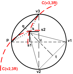
The computation of the probability $P_{1}$ is illustrated in figure 2. Nodes $v_{i}$, for $i\in[1,3]$, should belong to $\mathcal{D}(u,2R)\setminus\mathcal{D}(u,R)$ and should be at a distance belonging to $(3R,4R]$ from each other. To maximize the number of possible nodes $v_{3}$, we take $v_{1}\in\mathcal{C}(u,2R)$. The choice of $v_{1}$ done, we increase the number of possible nodes $v_{3}$ by taking $v_{2}\in\mathcal{C}(u,2R)\cap\mathcal{C}(v_{1},3R)$, approximating $3R+\varepsilon$ by $3R$. We make $v_{1}$ and $v_{2}$ closer increasing again the possibilities for $v_{3}$ by transforming the triangle $(v_{1},u,v_{2})$ in a right triangle. We then have $d(v_{1},v_{2})=2R\sqrt{2}$ computed as the hypotenuse in the triangle $(u,v_{1},v_{2})$. We now select $v_{3}$ that belongs to $\mathcal{D}(u,2R)\setminus\mathcal{D}(u,R)\setminus\mathcal{D}(v_{1},2R\sqrt{2})\setminus\mathcal{D}(v_{2},2R\sqrt{2})$, corresponding to the hatched area depicted in Figure 1. We compute $S_{P}$ the surface of this area. $S_{P}\leq S_{D}-2S_{T}-S_{C}$, where $S_{D}$ is the surface of the disk quarter $\mathcal{D}(u,2R)$, $S_{T}$ is the surface of the triangle formed by $s$, $u$ and $v_{3}$ and $S_{C}$ the surface of the square $(s,s_{1},u,s_{2})$ whose diagonal is $y$ (see figure 1). We first compute $d(u,q)$ in the right triangle $(u,q,v_{3})$. We get $2R^{2}+d(u,q)^{2}=2^{2}R^{2}$. Hence, $d(u,q)=R\sqrt{2}$. In the isosceles triangle $(v_{1},v_{2},s)$, we compute $d(q,t$. We have: $(d(s,t))^{2}+2R^{2}=8R^{2}$. Since $d(s,t)=d(s,u)+d(u,q)$, we get $d(s,u)=d(s,t)-d(u,q)=(\sqrt{6}-\sqrt{2})R$. We then get:
$S_{D}=\Pi R^{2}$ and $S_{C}=y^{2}/2=(4-2\sqrt{3})R^{2}$.
$S_{T}=(\sqrt{4-2\sqrt{3}}-2+\sqrt{3})R^{2}$.
We deduce $S_{P}=(\Pi-2\sqrt{4-2\sqrt{3}})R^{2}$.
Hence, $P_{1}=\frac{number\ of\ favorable\ cases}{number\ of\ possible\ cases}=\frac{S_{P}}{4\Pi R^{2}}$.
Finally, we get $P_{1}=\frac{1}{4}-\frac{\sqrt{4-2\sqrt{3}}}{2\Pi}$.

References

- [1] V. Vizing, On an estimate of the chromatic class of a p-graph, Diskret. Analiz., 3:23-30, 1964.
- [2] M. Garey, D. Johnson, Computers and intractability: a guide to theory of NP-completeness, W.H. Freeman, San Francisco, California, 1979.
- [3] S. T. McCormick, Optimal approximation of sparse Hessians and its equivalence to a graph coloring problem, Math. Programming, v26, pp. 153-171, 1983.
- [4] I. Amdouni, P. Minet, C. Adjih, Node coloring for dense wireless sensor networks, INRIA Research report RR-7588, http://hal.inria.fr/inria-00582457/PDF/RR-7588.pdf, March 2011.
- [5] M. Hilgemeier, N. Drechsler, R. Drechsler, Fast heuristics for the edge coloring of large graphs, Euromicro Symposium on Digital system design, DSD’03, IEEE computer Society, 2003.
- [6] P. Galinier, A. Hertz, A survey of local search methods for graph coloring, Computers & Operations Research, 3(9), 2547-2562, September 2006.
- [7] Q. Wu, J.K. Hao, Coloring large graphs based on independent set extraction, to appear in Computers and Operations Research, Elsevier, 2011.
- [8] I. Cargiannis, A. Fishkin, C. Kaklamanis, E. Papaioannou, A tight bound for online coloring of disk graphs, Theoretical Computer Science, 384, 2007.
- [9] B. Clark, C. Colbourn, and D. Johnson, “Unit disk graphs”, Discrete Mathematics, Vol. 86, Issues 1-3, Dec. 1990
- [10] J.C. Bermond, F. Havet, F. Huc, C. Linhares-Sales, Improper colouring of weighted grid and hexagonal graphs, Discrete Mathematics, Algorithms and Applications, 2(3):395-411, 2010.
- [11] V. Rajendran, K. Obraczka, J.J. Garcia-Luna-Aceves, Energy-efficient, collision-free medium access control for wireless sensor networks, Sensys’03, Los Angeles, California, November 2003.
- [12] I. Rhee, A. Warrier, M. Aia, J. Min, Z-MAC: a hybrid MAC for wireless sensor networks, SenSys’05, San Diego, California, November 2005.
- [13] P. Minet, S. Mahfoudh, SERENA: SchEduling RoutEr Nodes Activity in wireless ad hoc and sensor networks, IWCMC 2008, IEEE International Wireless Communications and Mobile Computing Conference, Crete Island, Greece, August 2008.
- [14] V. Rajendran, J.J. Garcia-Luna-Aceves, K. Obraczka, Energy-efficient, application-aware medium access for sensor networks, IEEE MASS 2005, Washington, November 2005.
- [15] W. Lee, A. Datta, R. Cardell-Oliver, FlexiTP: a flexible-schedule-based TDMA protocol for fault-tolerant and energy-efficient wireless sensor networks, IEEE Transactions on Parallel and Distributed Systems, vol. 19, 6, June 2008.
- [16] S. Gobriel, D. Mosse, R. Cleric, TDMA-ASAP: sensor network TDMA scheduling with adaptive slot stealing and parallelism, ICDCS 2009, Montreal, Canada, June 2009.
- [17] M. Hassan, A. Chickadel, A review of interference reduction in wireless networks using graph coloring methods, GRAPH-HOC, 3(1), March 2011.
- [18] S. Mahfoudh, G. Chalhoub, P. Minet, M. Misson, I. Amdouni, Node Coloring and Color Conflict Detection in Wireless Sensor Networks, Future Internet 2010, 2(4), 469-504, October 2010.
- [19] Ta Xiaoyuan, Mao Guoqiang, B.D.O. Anderson, On the Probability of K-hop Connection in Wireless Sensor Networks IEEE Communications Letters, Volume 11 Issue 8, pp 662 - 664, August 2007