Finite Alphabet Control of Logistic Networks with Discrete Uncertainty
Abstract
We consider logistic networks in which the control and disturbance inputs take values in finite sets. We derive a necessary and sufficient condition for the existence of robustly control invariant (hyperbox) sets. We show that a stronger version of this condition is sufficient to guarantee robust global attractivity, and we construct a counterexample demonstrating that it is not necessary. Being constructive, our proofs of sufficiency allow us to extract the corresponding robust control laws and to establish the invariance of certain sets. Finally, we highlight parallels between our results and existing results in the literature, and we conclude our study with two simple illustrative examples.
1 Introduction
Production networks, distribution networks and transportation networks are all instances of logistic networks, essentially dynamic network flow problems in which the inventories, controlled flows, supplies and demands evolve in time. The dynamics of these systems are linear: The state of the system represents accumulated products in production stages, inventory stored in warehouses, or commodities available at hubs. The control inputs represent the controlled flows between these production stages, warehouses or hubs, such as production processes or transportation routes. The disturbance inputs represent fluctuating supplies of raw materials as well as unknown consumer demands. Practically, excess inventory results in undesirable holding costs, while shortages result in disruptions in the production or supply chain and a potential loss of clients. In view of this tradeoff, it is desirable to maintain inventory in all parts of the network within reasonable bounds in spite of the operating uncertainty.
In this context, questions of stability, reachability and robustness naturally arise. Such questions have been previously considered in the control literature on production-distribution or multi-storage systems where the unknown but bounded disturbances as well as the control inputs are assumed to take values in analog sets, and the invariant sets of interest range from hyperboxes to polytopes, ellipsoids, and more generally, convex sets [13, 12, 11, 10, 4]. Related research directions in operations research address optimization problems in uncertain, multi-period inventory models. For instance, base stock policies can be interpreted in terms of guaranteeing upper bounds on robustly control invariant sets. Traditionally, cost functions penalizing holding and storage costs are used in conjunction with dynamic programming techniques to robustly maintain the stock within a neighborhood of zero. In a bid to overcome the dimensionality problems inherent in dynamic programming and to mitigate undesirable dynamics, robust optimization based approaches [8] such as Affinely Adjustable Robust Counterpart (AARC) methods, Globalized Robust Counterpart (GRC) methods [5], and various extensions, have been developed. In the supply chain literature, the network topology is often restricted to a tree, chain, or other special structure that can be exploited in the solution.
Robustly control invariant sets have also been studied in a more general control context due to their relevance to a variety of control problems, including constrained control and robust model predictive control. Early results exploited dynamic programming techniques to characterize invariant sets [7], and derived necessary and sufficient conditions for robust control invariance, expressed in terms of set equalities [6]. An in-depth survey of the existing body of literature in control, emphasizing techniques that exploit connections with control Lyapunov functions, dynamic programing, and classical analytical results can be found in [9]. More recent characterizations of robustly control invariant sets for discrete-time linear systems were proposed in [17], allowing for tractable, convex-optimization based analysis approaches.
In this paper, we consider discrete-time dynamic network flow problems in which the inputs are restricted to take their values in finite alphabets, and we focus on a class of polytopic invariant sets (hyperboxes). We seek to address the following two questions: Under what conditions does a robustly control invariant hyperbox exist? And under what conditions is such a set robustly globally attractive? We present two main results: First, we derive a necessary and sufficient condition for the existence of robustly control invariant hyperboxes. Second, we show that a stricter version of this condition is sufficient, though not necessary in general, to guarantee robust global convergence of all state trajectories to the invariant set. While the problems are posed as existence questions, our results touch on analysis and synthesis problems as well. As the proposed proofs of sufficiency are constructive, they allow one to immediately extract the corresponding robust control laws. Moreover, they establish sufficient conditions for verifying invariance of certain sets. Finally, we highlight connections between our derived results and existing ones in the literature for the traditional setting.
The novelty in our setup, which distinguishes it from most of the above referenced literature, is in the discrete nature of the control and disturbance inputs in conjunction with set based models of uncertainty. Discrete action spaces are justifiable from both practical and theoretical perspectives: From a practical standpoint, goods are usually processed, transported and distributed in batches. From a theoretical standpoint, the study of systems under discrete controls and disturbances has sparked much interest in recent years as evidenced by the literature on finite alphabet control [14, 19, 20, 18], mixed integer model predictive control [1], discrete team theory [21] and boolean control [3] where the problems of interest are often formulated as min-max games [2]. Note that while the setup in [6] is general enough to allow discrete inputs, our derivation differs significantly as do our proposed conditions, being stated explicitly in terms of conditions on the alphabet sets rather than set equivalence conditions.
Organization: We present the problem statement in Section 2.1 and explain its practical significance in Sections 2.2 and 2.3. We state the main results in Section 3, present complete proofs in Section 4, discuss connections to the existing literature in Section 5, present simple illustrative examples in Section 6, and conclude with directions for future work in Section 7.
Notation: , , and denote the reals, integers, non-negative reals and non-negative integers, respectively. denotes the component of , while denotes the vector in whose entries are all equal to one. and denote the convex hull and interior, respectively, of . denotes the set of vertices of the unit hypercube, that is . For , , denotes the image of by , that is . Given a set , denotes its set of vertices, that is .
2 Problem Setup
2.1 Problem Statement
Consider the system described by
| (1) |
where , state , control input and disturbance input . The control and disturbance alphabet sets and , respectively, are ordered with and . , are given. This system is a fairly general model of a logistic network, as we will describe in Section 2.2.
Definition 1.
A hyperbox is robustly control invariant if there exists a control law such that for every , for any disturbance .
Remark 1.
When is robustly control invariant, then so is any other hyperbox . Indeed, control law defined by , where , verifies this assertion.
Definition 2.
A hyperbox is robustly globally attractive if there exists a control law such that for every initial condition and disturbance , the corresponding state trajectory satisfies for some .
We are interested in answering two questions for the system described in (1):
Question 1: Under what conditions does a robustly control invariant hyperbox exist?
Question 2: Under what conditions does a robustly globally attractive and control invariant hyperbox exist?
2.2 Relevance of the Model
The dynamics in (1) constitute a unified and fairly general abstract model of logistic networks such as production networks, distribution networks and transportation networks.
For instance, a production system consists of products in one of several possible forms (raw products, intermediate products or finished products), together with various production processes by which a product is transformed, or several products are combined, to yield a new intermediate or final product. This production system can be modeled as a network in which the products are represented as nodes while the production processes are represented by (weighted) hyper-arcs. These production processes are typically individually controlled by the operator of the network: The hyper-arcs are thus associated with control inputs. Additionally, the network may interact with its external environment through both controlled and uncontrolled flows representing generally uncertain supplies of raw material as well as demands of various finished products. In the mathematical model (1) of this production network, the state vector represents the amounts of the various products available in the network at time : Specifically, represents the amount of product in the network at time . The ‘’ term encodes the production processes and nominal supplies, and the rate at which they proceed, controlled by the network operator. The ‘’ term, in contrast, encodes uncertain supplies and demands, or possibly uncertainty in the production processes. Specifically, matrices and represent the network topology, with non-zero entries indicating hyper-arcs and their weights and/or locations of external flows. Inputs and represent the controlled and uncontrolled flows, respectively. The amount of product at the end of a production cycle thus equals the amount available at the beginning of the production cycle, plus any amounts produced, minus any amounts depleted during the production cycle.
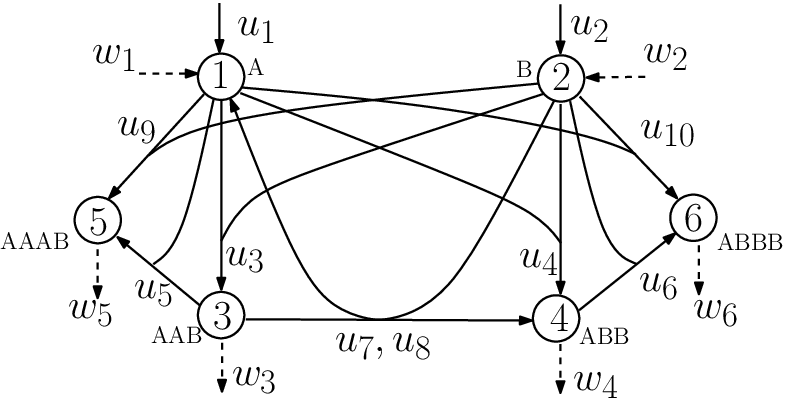
To make things more concrete, consider a chemical production system in which 2 raw products, referred to here as products A and B, can be used to produce 4 finished products, say AAAB, AAB, ABB and ABBB. This production system can be described by a network with 6 nodes, each representing one of the 6 products, as shown in Figure 1. Final product AAAB (represented by node 5 in the network) can be obtained through one of 2 production processes, namely by combining products A and B in a 3:1 ratio, or by combining products A and AAB in a 1:1 ratio. These two processes are represented by 2 hyper-arcs incoming into node 5 in Figure 1, and are associated with control inputs and , respectively, as shown. In contrast, product ABB (represented by node 4 in the network) can be produced by combining raw materials A and B in a 1:2 ratio, or from product AAB by releasing one unit of A and adding one unit of B. These two processes are represented by two hyper-arcs associated with control inputs and , respectively. Likewise, the two other finished products can be obtained by various production processes represented by hyper-arcs in the network, and associated with control inputs , and . The supply of raw products A and B is uncertain, represented by nominal flow rates associated with control inputs and and fluctuations in supply rates associated with disturbance inputs and . The demand for the 4 finished products is uncertain, represented by disturbance inputs through . The matrix of the mathematical model describing this network is given by:
| (2) |
In this representation, the column of the matrix represents the hyper-arc associated with control input : For instance, the hyper-arc associated with input is represented by column 9. The non-zero entries of the column indicate that three units of product A (represented by node 1) and one unit of product B (represented by node 2) and used to produce one unit of product AAAB (represented by node 5). As such, matrix encodes the topology of the network, namely the hyper-arcs and their weights. Similarly, the matrix is given by:
| (3) |
Likewise in the case of distribution and transportation networks, the nodes of the network represent warehouses and transportation hubs, respectively, with the component of the state vector thus representing the quantity of commodities present at the warehouse/hub. The ‘’ term encodes the various transportation routes, distribution protocols, supplies and demands, with matrices , representing the network topology and inputs and again respectively representing the controlled flows and uncertainty in the system.
2.3 Relevance of the Problem Statement
In this setting, it is intuitively desirable to contain each component of the state vector within two bounds, a zero lower bound and a positive upper bound. The zero lower bound guards against shortages and interruptions in the production process, or against the underuse of distribution and transportation resources. The upper bound ensures that the storage capabilities of the system are not exceeded. The question of existence of robustly control invariant sets, specifically hyperboxes (Question 1 in Section 2.1), thus naturally arises.
Moreover in this setting, the model of uncertainty (specifically the choice of set ) encodes the typical uncertainty encountered in day to day operations. Since it is impossible to rule out rare occurrences of large unmodeled uncertainty that would drive the system away from its typical operation, such as emergencies or catastrophic events, it is reasonable to question whether the system can recover from such events: The question of robust global attractivity of the robustly control invariant hyperboxes (Question 2 in Section 2.1) thus also naturally arises.
3 Main Results
Consider the following sets defined for :
Associate with every a signature, namely an n-tuple with if and if , and two subsets of defined by
We can now state the main results. The first provides a complete answer to Question 1:
Theorem 1.
The following two statements are equivalent:
- (a)
There exists a set that is robustly control invariant.
- (b)
The following condition holds
(4)
The second proposes a sufficient condition for the existence of a robustly control invariant set that is globally attractive, thus giving a partial answer to Question 2. In general, this condition need not be necessary as discussed in Section 4.
Theorem 2.
If the following condition holds
| (5) |
there exists a robustly control invariant and globally attractive set .
Remark 2.
While it is somewhat disappointing that both conditions and are combinatorial in nature, and thus grow exponentially with the number of nodes in the network, the result is not surprising in view of the established results for the case of analog alphabets. Indeed in [13, 10], discrete-time networks subject to analog control inputs and disturbances were analyzed. For instance, it was shown that when , for some scalars , , the condition
is necessary and sufficient for the existence of a globally attractive robustly control invariant set. While this condition appears deceptively simple, verifying it is known to be NP-hard: Indeed, it requires checking constraints [13] in general.
4 Derivation of the Main Results
4.1 Existence of a Robustly Control Invariant Set
We begin by establishing a necessary condition for a given control law to render a set robustly control invariant.
Lemma 1.
Let be robustly control invariant, and consider a control law as in Definition 1. Then at every vertex , we have
where is the unique element of whose signature is identical to that of .
Proof.
Assume that for some with signature , and consider a set , . Pick a . By assumption, there exists an such that . Now letting and applying control input , we have , and satisfies
for some when and
for some when . Hence for some . Noting that the choice of was arbitrary allows us to conclude that is not robustly control invariant. ∎
Lemma 2.
If the following condition holds
the set is robustly control invariant for any choice whenever .
Proof.
Assume that holds for all and pick for each a control input . The set is robustly control invariant. Indeed, consider the control law defined by , where is the unique vertex of the unit hypercube with signature if and otherwise. Note that under this control law, we have for every
Thus by construction, when , and . Likewise when , and . It follows that is robustly control invariant. ∎
Remark 3.
Note that when the sufficient condition (4) holds, our proof effectively provides an immediate construction of a full state feedback control law rendering any sufficiently large hyper box robustly control invariant. For any choice of , , the corresponding robustly control invariant set can be interpreted as an outer set (or superset) of the smallest robustly control invariant set.
We are now ready to prove Theorem 1:
Proof of Theorem 1: (a) (b): Assume that for some with signature , consider a set , , and pick vertex with signature . For any control law , we necessarily have (as the latter set is empty). Noting that the choice of control law was arbitrary allows us to conclude that is not robustly control invariant. Noting that the choice of was arbitrary allows us to conclude that a robustly control invariant set cannot exist, thus completing our argument.
(b) (a): Follows directly from Lemma 2 which provides an explicit construction for such a set.
4.2 Robust Global Attractivity
We begin by establishing sufficient conditions for a set to be robustly globally attractive. Our proof hinges on the construction of an appropriate Lyapunov-like function.
Lemma 3.
If the following condition holds
set with is robustly globally attractive for any choice .
Proof.
Pick a choice , for . To prove global attractiveness of the corresponding set , consider the control law defined by , where is the unique vertex of the unit hypercube with signature if and otherwise. Letting , note that . Consider the function defined by
Note that by construction, we have , for all and . Moreover, observe that under control law we have
| (6) |
along system trajectories whenever . To verify this, consider any , and consider the coordinate direction. We have:
| (7) |
with equality holding only in the case where the right hand side is zero. Indeed, we can distinguish three cases:
- •
: In this case, by construction we have , and
- •
: In this case, by construction we have , and
- •
: In this case, by construction we have , and
Equation (6) thus follows from the the fact that (7) holds for each , with equality only when both terms are identically 0.
Moreover, we have
| (8) |
whenever and .
We are now ready to prove Theorem 2:
Proof of Theorem 2: The proof is constructive. Assume that (5) holds and pick a choice , for . The set is robustly control invariant by Lemma 2, since . Moreover, is globally attractive by Lemma 3.
In the case of a degenerate network consisting of a single node (i.e. when , and arbitrary), condition (5) is necessary as well as sufficient for robust global attractivity:
Proposition 1.
When , if for some , there cannot exist a set that is robustly globally attractive.
Proof.
Assume, without loss of generality, that and consider a set . It follows that for any and any choice of control law, for some , call this . We can thus always find a disturbance input, namely , , for which any state trajectory initialized to the right of the interval will remain to the right of the interval for all times, and is not robustly control invariant. ∎
In general, however, condition (5) is not necessary for global attractivity. Indeed, consider the second order counterexample constructed as follows:
Counterexample 1.
Let , , , , , and . In this case, we have four possible control inputs,
Computing the relevant sets, we get
On the unit hypercube, we have
By Lemma 2, there exists a set that is robustly control invariant, namely . While condition (5) does not hold, it is easy to note that is also robustly globally attractive. Indeed, consider the control law defined by
It is straightforward to verify that renders robustly control invariant and globally attractive.
5 Discussion
In this Section, we establish connections between our results and existing results, focusing in particular on certain set inclusion conditions that often appear in the literature on set invariance in control.
5.1 Connections to Set Inclusion Conditions on the Alphabet Sets
The necessary and sufficient condition for existence of a robustly control invariant set, as well as the sufficient condition for global attractivity are both formulated in terms of combinatorial conditions. In contrast, conditions derived in the literature for the existence of robustly control invariant sets for discrete-time dynamic network flow models with analog-valued inputs are typically presented as set inclusion conditions. Specifically in [13] the authors prove that
| (12) |
is necessary and sufficient for a robustly control invariant set to exist. In light of this, in this section we attempt to connect our combinatorial conditions with appropriate set inclusion conditions. In particular, we show that (4) implies another condition, formulated in terms of the convex hull of and . Likewise, we show that (5) implies another condition, formulated in terms of the interior of the convex hull of and the convex hull of .
However, it should be emphasized that this exercise is mainly academic for two reasons: First, set inclusion conditions (12) are known to be NP-hard to verify in general. Indeed, verifying the condition when and are closed convex sets requires checking constraints in general, where is the dimension of the underlying state-space. This characterization, which relies on an earlier result in [15], is stated and proved in Section 4 of [13]. As such, set inclusion conditions do not offer much promise of a substantial reduction in computational burden. Second, the directions of the implications are such that a set inclusion condition can only be used to conclude the non-existence of a robustly control invariant set in the case where the condition is violated.
Lemma 4.
Condition (4) holds iff for each closed orthant , , there exists a control input such that the set
satisfies .
Proof.
Follows from the definitions by noting that each vertex of can be uniquely associated with an orthant in , namely the unique orthant containing . ∎
Lemma 5.
Condition (5) holds iff for each open orthant , , there exists a control input such that the set
satisfies .
Proof.
Follows from the definitions by noting that each vertex of can be uniquely associated with an orthant in , namely the unique orthant containing . ∎
Theorem 3.
Proof.
When (4) holds, by Lemma 4 we have that for each closed orthant , there exists a such that . Let . Pick any . We have (with some abuse of notation)
Since the choice of was arbitrary in , we conclude that for any there exists such that . Hence , and .
When , both implications in the above derivation become equivalences (the second by picking to correspond to extremal points), and the converse statement holds. ∎
Theorem 4.
Proof.
When (5) holds, by Lemma 5 we have that for each open orthant , there exists a such that . Let . Pick any . We have (again with some abuse of notation)
Since the choice of was arbitrary in , we conclude that for any there exists such that . Hence , and .
When , both implications in the above derivation become equivalences (the second by picking to correspond to extremal points), and the converse statement holds. ∎
5.2 Connections to Sub-Tangentiality Conditions
Lemma 1 can be interpreted as a counterpart to the necessary condition in Nagumo’s Theorem [16], adapted to the discrete-time, forced, and discrete alphabet setting of interest here. Nagumo’s sub-tangentiality condition and related conditions (see [9] for an overview), while known to be sufficient for continuous-time systems and linear discrete-time systems under analog inputs, are not sufficient for general discrete-time systems. As such, it is not surprising that additional constraints need to be placed on the set to ensure sufficiency of condition (4) in establishing set invariance.
6 Illustrative Examples
We begin with a simple scalar example for intuition. We then revisit the production network introduced in Section 2.2.
6.1 A Scalar Example
Consider the scalar dynamics () given by
with alphabets and . We begin by computing sets and (no need for indices ‘’ in this case) by inspecting Table 1 whose entries are simply the values of ‘’: This table can be interpreted as the payoff matrix of a zero sum game between players and .
We have and iff
We thus conclude that a robustly control invariant set indeed exists iff , and is moreover globally attractive provided strict equality holds. Consider for example the case where , for which a robustly control invariant set is guaranteed to exist: It is straighforward to verify that is robustly control invariant (it is in fact the smallest such set).
6.2 A Six Node, Ten Arc Production Network
We revisit the production process described in Section 2.2 and represented by the network in Figure 1. We have , , , and matrices and are given in (2) and (3), respectively. In this example, we assume that , representing the operator’s ability to completely shut down a production process or determine its rate up to some maximum level. We assume that .
Under these assumptions, condition (5) holds. We proceed to verify this without explicitly constructing the sets , by employing a heuristic approach. Indeed, we solve the following linear program with decision variables and for each vertex :
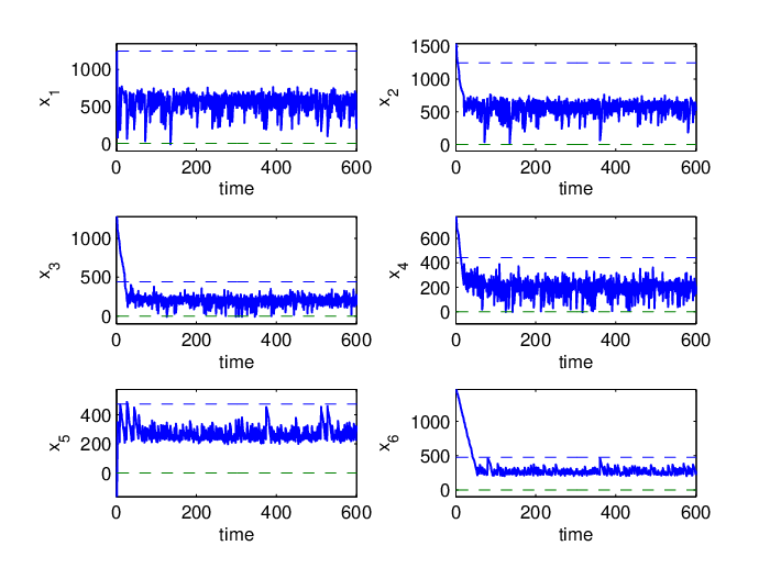
where is a chosen parameter. Note that the linear program returns a fractional solution that can be rounded to an integer solution within the admissible input set. Also note that the existence, for each choice of , of an integer solution satisfying the first four LP constraints (for any ) effectively ensures satisfaction of (5), since these constraints represent extremal (worst case) values of the disturbance inputs. Parameter allows us some flexibility in applying this heuristic: A larger translates into a higher likelihood that the rounded integer solution will satisfy the desired constraints, at the expense of missing potential solutions if is too large. Once we identify rounded integer controls and double check that condition (5) still holds, we store these values in a look-up table ready to be implemented in feedback form, chosen in agreement with the control law proposed in the proof of Lemma 3. Having chosen the feedback law, we can now also compute the robustly globally attractive control invariant set : The obtained values are displayed in Table 2, and are indicated by the dashed blue lines in Figure 2.
Having computed the feedback control law offline, we report on Monte Carlo simulations of the closed loop system. We ran 30 different paths with 600 samples (horizon steps) each starting from uniformly randomly selected initial states in the interval and with random demand uniformly drawn from the admissible intervals. The first sample path starting from initial state is depicted in Fig. 2, with the dashed lines delineating the invariant hyperbox. All simulations are carried out with MATLAB on an Intel(R) Core(TM)2 Duo CPU P8400 at 2.27 GHz and 3GB of RAM. The run time of the offline computation of the control law is less than 5 seconds, while the run time of loading all the controls in the look-up table and running the Monte Carlo simulations is about 12 seconds.
7 Conclusions & Future Work
We considered logistic networks in which the control and disturbance inputs take their values in finite sets. We established a necessary and sufficient condition for the existence of robustly control invariant hyperboxes, and we showed that a stronger version of this condition is sufficient, albeit not necessary in general, to guarantee robust global attractivity. The proposed conditions are combinatorial in nature, which is not surprising as the problem is known to be NP-hard even when the input signals are analog.
Future work will focus on deriving bounds on the size of the smallest such invariant hyperboxes, as well as considering more interesting models of finite alphabet uncertainty.
8 Acknowledgments
D. C. Tarraf’s research was supported by NSF CAREER award ECCS 0954601 and AFOSR Young Investigator award FA9550-11-1-0118. D. Bauso’s research was supported by the 2012 “Research Fellow” Program of the Dipartimento di Matematica, Universitá di Trento and by the PRIN 20103S5RN3 “Robust decision making in markets and organization.”
References
- [1] D. Axehill, L. Vandenberghe, and A. Hansson, “Convex relaxations for mixed integer predictive control,” Automatica, vol. 46, no. 5, pp. 1540–1545, June 2010.
- [2] T. Basar and G. Olsder, Dynamic Noncooperative Game Theory. SIAM, 1999.
- [3] D. Bauso, “Boolean-controlled systems via receding horizon and linear programming,” Journal of Mathematics of Control, Signals and Systems, vol. 21, no. 1, pp. 69–91, 2009.
- [4] D. Bauso, L. Giarrè, and R. Pesenti, “Robust control of uncertain multi-inventory systems via linear matrix inequality,” International Journal of Control, vol. 83, no. 8, pp. 1723–1740, 2010.
- [5] A. Ben-Tal, B. Golany, and S. Shtern, “Robust multi-echelon multi-period inventory control,” European Journal of Operational Research, vol. 199, no. 3, pp. 922–935, 2009.
- [6] D. P. Bertsekas, “Infinite-time reachability of state-space regions by using feedback control,” IEEE Transactions on Automatic Control, vol. 17, no. 5, pp. 604–613, 1972.
- [7] D. P. Bertsekas and I. B. Rhodes, “On the minmax reachability of target sets and target tubes,” Automatica, vol. 7, pp. 233–247, 1971.
- [8] D. Bertsimas and A. Thiele, “A robust optimization approach to inventory theory,” Operations Research, vol. 54, no. 1, pp. 150–168, 2006.
- [9] F. Blanchini, “Set invariance in control,” Automatica, vol. 35, no. 11, pp. 1747–1767, 1999.
- [10] F. Blanchini, S. Miani, R. Pesenti, F. Rinaldi, and W. Ukovich, “Robust control of production-distribution systems,” in Perspectives in Robust Control, ser. Lecture Notes in Control and Information Sciences, S. O. R. Moheimani, Ed. Springer, 2001, vol. 268, pp. 13–28.
- [11] F. Blanchini, S. Miani, and W. Ukovich, “Control of production-distribution systems with unknown inputs and system failures,” IEEE Transactions on Automatic Control, vol. 45, no. 6, pp. 1072–1081, June 2000.
- [12] F. Blanchini, F. Rinaldi, and W. Ukovich, “Least inventory control of multi-storage systems with non-stochastic unknown input,” IEEE Transactions on Robotics and Automation, vol. 13, no. 5, pp. 633–645, 1997.
- [13] ——, “A network design problem for a distribution system with uncertain demands,” SIAM Journal on Optimization, vol. 7, no. 2, pp. 560–578, May 1997.
- [14] G. C. Goodwin and D. E. Quevedo, “Finite alphabet control and estimation,” International Journal of Control, Automation and Systems, vol. 1, no. 4, pp. 412–430, 2003.
- [15] S. T. McCormick, “Submodular containment is hard, even for networks,” Operations Research Letters, vol. 19, pp. 95–99, 1996.
- [16] M. Nagumo, “Über die lage der integralkurven gewöhnlicher differentialgleichungen,” Proceedings of the Physico-Mathematical Society of Japan, vol. 24, pp. 551–559, 1942.
- [17] S. V. Rakovic, E. Kerrigan, D. Mayne, and K. I. Kouramas, “Optimized robust control invariance for linear discrete-time systems: Theoretical foundations,” Automatica, vol. 43, no. 5, pp. 831–841, 2007.
- [18] D. C. Tarraf, “A control-oriented notion of finite state approximation,” IEEE Transactions on Automatic Control, vol. 56, no. 12, pp. 3197–3202, December 2012.
- [19] D. C. Tarraf, A. Megretski, and M. A. Dahleh, “Finite approximations of switched homogeneous systems for controller synthesis,” IEEE Transactions on Automatic Control, vol. 56, no. 5, pp. 1140–1145, May 2011.
- [20] D. C. Tarraf, A. Megretski, and M. Dahleh, “A framework for robust stability for systems over finite alphabets,” IEEE Transactions on Automatic Control, vol. 53, no. 5, pp. 1133–1146, June 2008.
- [21] P. R. D. Waal and J. H. V. Schuppen, “A class of team problems with discrete action spaces: Optimality conditions based on multimodularity,” SIAM Journal on Control and Optimization, vol. 38, no. 3, pp. 875–892, 2000.