Semileptonic to decays at nonzero recoil with 2+1 flavors of improved staggered quarks
Abstract:
The Fermilab Lattice-MILC collaboration is completing a comprehensive program of heavy-light physics on the MILC (2+1)-flavor asqtad ensembles with lattice spacings as small as 0.045 fm and light-to-strange-quark mass ratios as low as 1/20. We use the Fermilab interpretation of the clover action for heavy valence quarks and the asqtad action for light valence quarks. The central goal of the program is to provide ever more exacting tests of the unitarity of the CKM matrix. We give a progress report on one part of the program, namely the analysis of the semileptonic decay to at both zero and nonzero recoil. Although final results are not presented, we discuss improvements in the analysis methods, the statistical errors, and the parameter coverage that we expect will lead to a significant reduction in the final error for from this decay channel.
July 10-16, 2011
Squaw Valley, Lake Tahoe, California
1 Introduction
Precision tests of the standard model from flavor factory and intensity frontier experiments can reveal new physics even if the accelerator energy isn’t sufficient to create the new particles associated with the new physics. Here preliminary results of a lattice-QCD calculation of the nonzero-recoil form factor for the semileptonic process are presented. The principal goal is to determine to a high precision. The theoretical uncertainty on limits the precision of the unitarity triangle constraint from neutral kaon mixing.
There are several methods for determining . (1) From the inclusive decay , perturbation theory and the operator product expansion provide an estimate of the inclusive decay rate, which is then combined with the measured decay rate to obtain [1]. (2) From the exclusive semileptonic decay , lattice-QCD methods provide the hadronic contribution to the decay rate [2]. For the special case of zero recoil, we have presented an unquenched calculation for this process three years ago [3] with a preliminary update reported at the Lattice 2010 [4] and CKM 2010 conferences [5] (3) Likewise, from the exclusive semileptonic decay , lattice-QCD methods provide the hadronic contribution [8]. Here we report the first unquenched lattice-QCD calculation for this process at nonzero recoil.
At present there is a 1.6 disagreement between the value of determined from inclusive decays and our recent preliminary value based on the decay at zero recoil, as illustrated in Fig. 1. Thus, further cross checks of and improvements in the theoretical calculations are needed. The value of can be determined from the ratio of the measured decay rate to the calculated hadronic form factor at any chosen recoil energy. Typically, the uncertainty in the experimental measurement increases as the recoil energy vanishes [12], whereas the uncertainty in the lattice-QCD calculation decreases [6, 7, 8]. Thus, to minimize the uncertainty in the ratio, it is best to combine results of the experimental measurement with those of the lattice-QCD calculation over the full range of available recoil energies. For this reason we undertake an analysis over a broad range.

2 Methodology for determining
The hadronic weak matrix element for this process is commonly parameterized as
| (1) |
Here, is velocity transfer, . The differential rate for the semileptonic decay is
| (2) |
where is defined as
| (3) |
Thus, once we know and , we can determine the form factor . Then, combining it with the result of the decay rate from experiment, we will obtain . In order to construct and , we need the following quantities:
| (4) | |||||
| (5) | |||||
| (6) | |||||
| (7) | |||||
| (8) |
where is the continuum hadronic weak vector current.
In our calculation we use the local (nonconserved) lattice vector current with improved heavy quark fields following [13], and we renormalize it following a partly nonperturbative method, namely
| (9) |
where the flavor-diagonal renormalization coefficients are computed nonperturbatively on the lattice via the conditions
| (10) | |||||
| (11) |
and is computed perturbatively [7]. Because of cancellations among similar loop diagrams, we expect that is nearly equal to 1 [7]. Preliminary results presented here omit the factor.
At zero recoil () we use the double ratio method [2]:
| (12) |
This ratio suppresses a large part of the statistical fluctuations, and it builds in the current renormalization .
3 Results
We report on results from an analysis of a large set of gauge field ensembles generated in the presence of flavors of improved staggered (asqtad) quarks [14, 15]. Further ensembles will be included in the future. Some key ensemble parameters are listed in Table 1.
| (fm) | size | |
|---|---|---|
| 0.15 | 0.2 | |
| 0.12 | 0.14 | |
| 0.12 | 0.2 | |
| 0.12 | 0.4 | |
| 0.12 | 0.1 | |
| 0.09 | 0.2 | |
| 0.09 | 0.15 |
| (fm) | size | |
|---|---|---|
| 0.09 | 0.1 | |
| 0.09 | 0.05 | |
| 0.06 | 0.2 | |
| 0.06 | 0.4 | |
| 0.06 | 0.14 | |
| 0.06 | 0.1 | |
| 0.045 | 0.2 |
On each ensemble we compute the three-point correlation functions relevant to the weak matrix elements and the two-point functions relevant to the propagation of the and mesons. For the heavy-light mesons we use heavy clover quarks in the Fermilab interpretation and light, improved staggered (asqtad) quarks [14, 15]. We use two types of interpolating operators for the and mesons, namely local and smeared using the 1S Richardson wave function. We set the valence-quark masses equal to the sea-quark masses. The bare lattice charm and bottom quark masses are fixed by matching the kinetic masses of the and mesons, respectively, to their experimental values. Some small adjustments will be needed to refine this tuning but are not yet included in this preliminary analysis.
In terms of interpolating operators and for the and mesons and the vector current, the two-point and three-point functions are given by
| (13) | |||||
| (14) |
where accounts for contributions that oscillate in , and is the lattice extent in the dimension. Note that in the three-point function above, we have put the meson at the origin and the meson at .
The matrix elements we want from Eq. (6) to Eq. (8) are obtained by factorization and reduction of the three-point functions. The reduction is based on the overlap coefficients , energies and masses obtained in fits to the two-point functions. For example, the matrix element is obtained from
| (15) |
in the limit and . In that limit it is a constant, , independent of . However, at finite and , complications from oscillating terms and excited states must be taken into account.
Because they contain a light staggered quark, the meson interpolating operators excite even- as well as odd-parity channels. The unwanted even-parity states manifest themselves as terms that oscillate in , corresponding to terms in the two-point and three-point functions with . To suppress the effect of the oscillating terms in the three-point functions, we average in both and (after removing the dominant exponential dependence on as in Eq. (15)) as follows:
| (16) |
Here, refers to any of the quantities derived from three-point functions, such as , , and .
Having suppressed the contributions of the oscillating states to the three-point correlators, we must still account for contributions from excited states. For example, for , the leading contributions are
| (17) |
where the primes indicate the overlaps and energies of the excited states of the same parity. We have neglected the doubly excited contribution, since the singly excited contribution is found already to be small. Thus, at finite and the ratio in Eq. (15) is not constant, but has a small contamination from excited states. We take this into account by fitting the resulting ratio to
| (18) |
as illustrated in Fig. 2. The fit parameter should be zero, but it is introduced to allow for a small error in determining and . The other terms involve and . These parameters are obtained from the fits of two-point functions. The results of two-point function fits then become prior central values and widths for fitting . We use a similar method to obtain and .

4 Chiral and continuum extrapolation
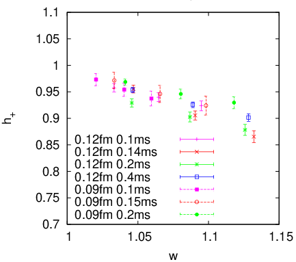
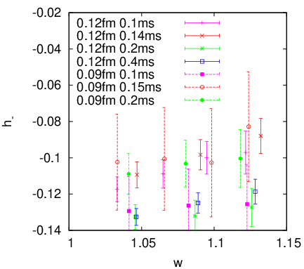
To complete the analysis we will extrapolate in the light quark masses to their physical values and take the continuum limit, using staggered chiral perturbation theory [16, 17] . At this preliminary stage, we don’t show physical values and chiral fit in this report. The numerical data points for and are shown in Fig. 3. We will need these data points to finish the extrapolation of physical value of and and the chiral fit.
5 Future plans
To complete the project, we need to (1) finish analyzing the available ensembles, (2) make adjustments for the tuning of the heavy quark masses, (3) compute the current renormalization ( factor), and (4) combine the experimental results for the differential decay rate with our results for the form factor to obtain , using methods employed for to extend over the full kinematic range [18].
Acknowledgments
Computations for this work were carried out with resources provided by the USQCD Collaboration, the Argonne Leadership Computing Facility, the National Energy Research Scientific Computing Center, and the Los Alamos National Laboratory, which are funded by the Office of Science of the U.S. Department of Energy; and with resources provided by the National Center for Supercomputing Applications and the National Institute for Computational Science, the Pittsburgh Supercomputer Center, the San Diego Supercomputer Center, and the Texas Advanced Computing Center, which are funded through the National Science Foundation’s Teragrid/XSEDE Program. This work was supported in part by the U.S. Department of Energy under Grants No. DE-FG02-91ER40664 (D.D.), No. DE-FG02-91ER40677 (D.D), and No. DE-FC06-ER41446(C.D.); and in part by the U.S. National Science Foundation under grants PHY0757333 (C.D.) and PHY0903571 (S.-W.Q.). J.L. is supported by the STFC and by the Scottish Universities Physics Alliance. This manuscript has been co-authored by employees of Brookhaven Science Associates, LLC, under Contract No. DE-AC02-98CH10886 with the U.S. Department of Energy. R.S.V. acknowledges support from BNL via the Goldhaber Distinguished Fellowship. D.D. was supported in part by the URA Visiting Scholars’ program at Fermilab. Fermilab is operated by Fermi Research Alliance, LLC, under Contract No. DE-AC02-07CH11359 with the United States Department of Energy.
References
- [1] C. G. Boyd, Z. Ligeti, I. Z. Rothstein, and M. B. Wise, Phys. Rev. D 55 (1997) 3027 [arXiv:hep-ph/9610518].
- [2] S. Hashimoto, A. S. Kronfeld, P. B. Mackenzie, S. M. Ryan, and J. N. Simone, Phys. Rev. D 66 (2002) 014503 [hep-ph/0110253].
- [3] C. Bernard et al. [Fermilab Lattice and MILC Collaborations], Phys. Rev. D 79 (2009) 014506 [arXiv:0808.2519 [hep-lat]].
- [4] J. A. Bailey et al. [Fermilab Lattice and MILC Collaborations], PoS LATTICE2010 (2010) 311 [arXiv:1011.2166 [hep-lat]].
- [5] P. B. Mackenzie, talk at Workshop on CKM Unitarity Triangle, Warwick, UK (September 2010).
- [6] A. S. Kronfeld, Phys. Rev. D 62 (2000) 014505 [hep-lat/0002008].
- [7] J. Harada, S. Hashimoto, A. S. Kronfeld, and T. Onogi, Phys. Rev. D 65 (2002) 094514 [hep-lat/0112045].
- [8] G. M. de Divitiis, E. Molinaro, R. Petronzio, N. Tantalo, Phys. Lett. B 655 (2007) 45 [arXiv:0707.0582 [hep-lat]].
- [9] J. Laiho, E. Lunghi, and R. S. Van de Water, Phys. Rev. D 81 (2010) 034503 [arXiv:0910.2928 [hep-ph]].
- [10] J. Laiho, E. Lunghi, and R. S. Van de Water, http://latticeaverages.org/, accessed July, 2011.
- [11] Heavy Flavor Averaging Group , http://www.slac.stanford.edu/xorg/hfag/semi/, accessed July, 2011.
- [12] J. E. Bartelt et al. [CLEO Collaboration], Phys. Rev. Lett. 82 (1999) 3746 [hep-ex/9811042].
- [13] A. X. El-Khadra, A. S. Kronfeld, P. B. Mackenzie, Phys. Rev. D 55 (1997) 3933 [hep-lat/9604004].
- [14] C. W. Bernard et al. [MILC Collaboration], Phys. Rev. D 61 (2000) 111502 [hep-lat/9912018].
- [15] A. Bazavov et al., Rev. Mod. Phys. 82 (2010) 1349 [arXiv:0903.3598 [hep-lat]].
- [16] C. K. Chow and M. B. Wise, Phys. Rev. D 48 (1993) 5202 [arXiv:hep-ph/9305229].
- [17] J. Laiho and R. S. Van de Water, Phys. Rev. D 73 (2006) 054501 [hep-lat/0512007].
- [18] J. A. Bailey et al. [Fermilab Lattice and MILC Collaborations], Phys. Rev. D 79 (2009) 054507 [arXiv:0811.3640 [hep-lat]].