A Computational Study of the Weak Galerkin Method for Second-Order Elliptic Equations
Abstract
The weak Galerkin finite element method is a novel numerical method that was first proposed and analyzed by Wang and Ye in [23] for general second order elliptic problems on triangular meshes. The goal of this paper is to conduct a computational investigation for the weak Galerkin method for various model problems with more general finite element partitions. The numerical results confirm the theory established in [23]. The results also indicate that the weak Galerkin method is efficient, robust, and reliable in scientific computing.
Keywords: finite element methods, weak Galerkin method
AMS 2000 Classification: 65N30
1 Introduction
In this paper, we are concerned with computation and numerical accuracy issues for the weak Galerkin method that was recently introduced in [23] for second order elliptic equations. The weak Galerkin method is an extension of the standard Galerkin finite element method where classical derivatives were substituted by weakly defined derivatives on functions with discontinuity. The weak Galerkin method is also related to the standard mixed finite element method in that the two methods are identical for simple model problems (such as the Poisson problem). But they have fundamental differences for general second order elliptic equations. The goal of this paper is to numerically demonstrate the efficiency and accuracy of the weak Galerkin method in scientific computing. In addition, we shall extend the weak Galerkin method of [23] from triangular and tetrahedral elements to rectangular and cubic elements.
For simplicity, we take the linear second order elliptic equation as our model problem. More precisely, let be an open bounded domain in , with Lipschitz continuous boundary . The model problem seeks an unknown function satisfying
| (1) |
where , , and are vector- and scalar-valued functions, as appropriate. Furthermore, assume that is a symmetric and uniformly positive definite matrix and the problem (1) has one and only one weak solution in the usual Sobolev space consisting of square integrable derivatives up to order one. and are given functions that ensure the desired solvability of (1).
Throughout the paper, we use to denote the standard norm over the domain , and use bold face Latin characters to denote vectors or vector-valued functions. The paper is organized as follows. In Section 2, the weak Galerkin method is introduced and an abstract theory is given. In particular, we prove that certain rectangular elements satisfy the assumptions in the abstract theory, and thus establish a well-posedness and error estimate for the corresponding weak Galerkin method with rectangular meshes. In Section 3, we present some implementation details for the weak Galerkin elements. Finally in Section 4, we report some numerical results for various test problems. The numerical experiments not only confirm the theoretical predictions as given in the original paper [23], but also reveal new results that have not yet been theoretically proved.
2 The Weak Galerkin Method
Let be a shape-regular, quasi-uniform mesh of the domain , with characteristic mesh size . In two-dimension, we consider triangular and rectangular meshes, and in three-dimension, we mainly consider tetrahedral and hexahedral meshes. For each element , denote by and the interior and the boundary of , respectively. Here, can be a triangle, a rectangle, a tetrahedron or a hexahedron. The boundary consists of several “sides”, which are edges in two-dimension or faces(polygons) in three-dimension. Denote by the collection of all edges/faces in .
On each , let be the set of polynomials on with degree less than or equal to , and be the set of polynomials on with degree of each variable less than or equal to . Likewise, on each , and are defined analogously. Now, define a weak discrete space on mesh by
Observe that the definition of does not require any form of continuity across element or edge/face interfaces. A function in is characterized by its value on the interior of each element plus its value on the edges/faces. Therefore, it is convenient to represent functions in with two components, , where denotes the value of on all s and denotes the value of on .
We further define an projection from onto by setting , where is the local projection of in , for , and is the local projection in , for .
The idea of the weak Galerkin method is to seek an approximate solution to Equation (1) in the weak discrete space . To this end, we need to introduce a discrete gradient operator on . Indeed, this will be done locally on each element . Let be a space of polynomials on such that ; details of will be given later. Let
A discrete gradient of is defined to be a function such that on each ,
| (2) |
where is the unit outward normal on . Clearly, such a discrete gradient is always well-defined.
Denote by the standard -inner product on . Let be a subset of consisting of functions with vanishing boundary values. Now we can write the weak Galerkin formulation for Equation (1) as follows: find such that on each edge/face and
| (3) |
for all . For simplicity of notation, we introduce the following bilinear form
| (4) |
The spaces and can not be chosen arbitrarily. There are certain criteria they need to follow, in order to guarantee that Equation (3) provides a good approximation to the solution of Equation (1). For example, has to be rich enough to prevent from the loss of information in the process of taking discrete gradients, while it should remain to be sufficiently small for its computational cost. Hence, we would like to impose the following conditions upon and :
-
(P1) For any and , if and only if on .
-
(P2) For any , where , we have
where and in what follows of this paper, denotes a generic constant independent of the mesh size .
Under the above two assumptions, it has been proved in [23] that Equation (3) has a unique solution as long as the mesh size is moderately small and the dual of (1) has an -regularity with some . Furthermore, one has the following error estimate:
| (5) | ||||
for any , and is the largest number such that the dual of Equation (1) has an -regularity.
There are several possible combinations of and that satisfy Assumptions (P1) and (P2). Two examples of triangular elements have been given in [23], which are
- 1.
Triangular element for . That is, in the definition of , we set . And in the definition of , we set and to be the th order Raviart-Thomas element [21].
- 2.
Triangular element for . That is, in the definition of , we set . And in the definition of , we set and , or in other words, the st order Brezzi-Douglas-Marini element [5].
The rest of this section shall extend this result to rectangular elements. An extension to three-dimensional tetrahedral and hexahedral elements is straightforward.
2.1 Weak Galerkin on Rectangular Meshes
Consider the following two type of rectangular elements:
- 1.
Rectangular element for . That is, in the definition of , we set . And in the definition of , we set and to be the th order Raviart-Thomas element on rectangle .
- 2.
Rectangular element for . That is, in the definition of , we set . And in the definition of , we set and to be the st order Brezzi-Douglas-Marini element on rectangle .
Denote by the space of polynomials with degree in and less than or equal to and , respectively, and . It is known that
and , . The degrees of freedom for are:
The degrees of freedom for are
It is also well-known that on each rectangle and each edge ,
| (6) | ||||||
Next, we show that the two set of elements defined as above satisfy Assumptions (P1) and (P2).
Lemma 1.
For the two type of rectangular elements given in this subsection, the Assumption P1 holds true.
Proof.
If on , then clearly vanishes since the right-hand side of (2) is zero from the divergence theorem. Now let us assume that . By (2) and using integration by parts, we have for all or ,
| (7) | ||||
We first consider the element . If , then is a constant on and clearly . If , take such that for all and let it traverse through all degrees of freedom defined by , for . Since and , Equation (7) gives , which implies that is a constant on . Now Equation (7) reduces into
Next, since for all , by letting traverse through all degrees of freedom on , we have on all . This implies in .
For the element, using the same argument as in the previous case, and noticing that , for all , we can similarly prove that in . ∎
Lemma 2.
For the two type of rectangular elements given in this subsection, the Assumption (P2) holds true.
Proof.
Let , . For any and , by (6) and the definition of projections, we have
In other words, on each , is the projection of onto or . Thus, the Assumption (P2) follows immediately from the approximation properties of the projection, and the fact that both and contains the entire polynomial space . ∎
3 Computation of Local Stiffness Matrices
Similar to the standard Galerkin finite element method, the weak Galerkin method (3) can be implemented as a matrix problem where the matrix is given as the sum of local stiffness matrices on each element . Thus, a key step in the computer implementation of the weak Galerkin is to compute element stiffness matrices. The goal of this section is to demonstrate ways of computing element stiffness matrices for various elements introduced in the previous sections.
For a given element , let , , be a set of basis functions for or , and , , be a set of basis functions for or . Note that is the union of basis functions from all edges/faces of element . Then every has the following representation in :
On each , the local stiffness matrix for Equation (3) can thus be written as a block matrix
| (8) |
where is an matrix, is an matrix, is an matrix, and is an matrix. These matrices are defined, respectively, by
where the bilinear form is defined as in (4), and , are the row and column indices, respectively.
To compute each block of , we first need to calculate the discrete gradient operator . For convenience, denote the local vector representation of by
Let , , be a set of basis functions for . Then, for every , its value on can be expressed as
Similarly, we denote the local vector representation of by
Then, by the definition of the discrete gradient (2), given , we can compute the vector form of on by
| (9) |
where the matrix , the matrix , and the matrix are defined, respectively, by
| (10) |
and
Notice that is a symmetric matrix.
Once the matrices , and are computed, we can use (9) to calculate the weak gradient of basis functions and on . It is not hard to see that
| (11) |
where and are the standard basis for the Euclidean spaces and , respectively, such that its -th entry is and all other entries are .
Define matrices
| (12) | ||||
where denote the standard inner-product on or , as appropriate. Clearly, is an matrix, is an matrix, and is an matrix. Then, an elementary matrix calculation shows that the local stiffness matrix for Equation (3) can be expressed in a way as specified in the following lemma.
Lemma 3.
The local stiffness matrix defined in (8) can be computed by using the following formula
| (13) | ||||
where the superscript stands for the standard matrix transpose.
For the Poisson equation , we clearly have and , . Since is symmetric, the local stiffness matrix becomes
| (14) |
In the rest of this section, we shall demonstrate the computation of the element stiffness matrix with two concrete examples.
3.1 For the Triangular Element
Let be a triangular element in . We consider the case when and being the lowest order Raviart-Thomas element. In other words, the discrete space consists of piecewise constants on the triangles, and piecewise constants on the edges of the mesh. In this case, the discrete gradient is defined by using the lowest order Raviart-Thomas element on the triangle . Clearly, we have , and .
Let , , be the vertices of the triangle and be the edge opposite to the vertex . Denote by the length of edge and the area of the triangle . We also denote by and the unit outward normal and unit tangential vectors on , respectively. Here should be in the positive (counterclockwise) orientation. If edge goes from vertex to and stays on the left when one travels from to , then it is not hard to see that
3.1.1 Approach I
One may use the following set of basis functions for the weak discrete functions on :
| (15) |
and
| (16) |
Notice that forms the standard basis for the lowest order Raviart-Thomas element, for which the degrees of freedom are taken to be the normal component on edges. Indeed, satisfies
It is straight forward to compute that, for the above defined basis functions,
The computation of is slightly more complicated, but it can still be done without much difficulty, especially with the help of symbolic computing tools provided in existing software packages such as Maple and Mathematica. For simplicity of notation, denote
Then, it can be verified that
| (17) | ||||
We point out that, the value of given as in (17) agrees with the one presented in [3]. A verification of the formula (17) can be carried out by using the following fact
In computer implementation, it is convenient to use a form for the local matrix that can be expressed by using only edge lengths, as the one given by (17).
In addition, using symbolic computing tools and the law of sines and cosines, we can write as follows:
Thus, to compute the local stiffness matrix , it suffices to calculate , and as given in (12), and then apply Lemma 3. Notice that these three matrices depend on the coefficients , and , and quadrature rules may be employed in the calculation. However, for the simple case of the Poisson equation , we see from (14) that
3.1.2 Approach II
We would like to present another approach for computing the local stiffness matrix in the rest of this subsection. Observe that a set of basis functions for the local space can be chosen as follows
| (18) |
where is the coordinate of the barycenter of . Note that both components of have mean value zero on . For the weak discrete function on , we use the same set of basis functions as given in (15). It is not hard to see that
and
Next, we use the formula (12) to calculate the matrices , and for the new basis (18). Finally, we calculate the local stiffness matrix by using the formula provided in Lemma 3.
Since the set of basis functions for the weak discrete space are the same in Approaches I and II, the resulting local stiffness matrix would remain unchanged from Approaches I and II. The set of basis functions (18) is advantageous over the set (16) in that the matrix is a diagonal one whose inverse in trivial to compute.
3.2 For the Cubic Element
Let be a rectangular box where are positive real numbers. We consider the three-dimensional cubic element, for which the discrete space consists of piecewise constants on and piecewise constants on the faces of . The space for the discrete gradient is the lowest order Raviart-Thomas element on . We clearly have , and .
Denote the six faces , by
Note that the volume of is given by and the normal direction to each face is given by
We adopt the following set of basis functions for the weak discrete space on
and
Clearly, each satisfies
It is not hard to compute that
and
Then, the local stiffness matrix can be computed using the formula presented in Lemma 3.
4 Numerical Experiments
In this section, we shall report some numerical results for the weak Galerkin finite element method on a variety of testing problems, with different mesh and finite elements. To this end, let and be the solution to the weak Galerkin equation (3) and the original equation (1), respectively. Define the error by where is the projection of onto appropriately defined spaces. Let us introduce the following norms:
where in the definition of , stands for the size of the element that takes as an edge/face. We shall also compute the error in the following metrics
Here the maximum norm is computed over all Gaussian points, and all other integrals are calculated with a Gaussian quadrature rule that is of high order of accuracy so that the error from the numerical integration can be virtually ignored.
4.1 Case 1: Model Problems with Various Boundary Conditions
First, we consider the Laplace equation with nonhomogeneous Dirichlet boundary condition:
| (19) |
We introduce a discrete Dirichlet boundary data , which is either the usual nodal value interpolation, or the projection of on the boundary. Let and define
When , we simply denote by . The discrete Galerkin formulation for the nonhomogeneous Dirichlet boundary value problem can be written as: find such that for all ,
We would like to see how the weak Galerkin approximation might be affected when the boundary data is approximated with different schemes (nodal interpolation verses projection). To this end, we use a two dimensional test problem with domain and exact solution given by . A uniform triangular mesh and the element is used in the weak Galerkin discretization. The results are reported in Table 1 and Table 2. It can be seen that both approximations of the Dirichlet boundary data give optimal order of convergence for the weak Galerkin method, while the projection method yields a slightly smaller error in and .
Next, we consider a mixed boundary condition:
where is the Dirichlet boundary data, is the Robin type boundary data, , and , . When , the Robin type boundary condition becomes the Neumann type boundary condition.
For the mixed boundary condition, it is not hard to see that the weak formulation can be written as: find such that for all ,
where denotes the inner-product on . We tested a two-dimensional problem with to be an identity matrix and with a uniform triangular mesh. The exact solution is chosen to be . This function satisfies
on the boundary segment . We use the Dirichlet boundary condition on all other boundary segments. The element is used in the discretization. For the Dirichlet boundary data, the projection is used to approximate the boundary data . The results are reported in Table 3. It shows optimal rates of convergence in all norms for the weak Galerkin approximation with mixed boundary conditions.
| 1/8 | 7.14e-01 | 2.16e-02 | 4.05e-02 | 1.01e+0 | 1.30e-01 | 4.43e-02 |
|---|---|---|---|---|---|---|
| 1/16 | 3.56e-01 | 5.61e-03 | 1.01e-02 | 5.04e-01 | 6.53e-02 | 1.12e-02 |
| 1/32 | 1.78e-01 | 1.41e-03 | 2.53e-03 | 2.51e-01 | 3.27e-02 | 2.86e-03 |
| 1/64 | 8.90e-02 | 3.55e-04 | 6.32e-04 | 1.25e-01 | 1.63e-02 | 7.15e-04 |
| 1/128 | 4.45e-02 | 8.88e-05 | 1.57e-04 | 6.29e-02 | 8.18e-03 | 1.79e-04 |
| 1.0012 | 1.9837 | 2.0014 | 1.0024 | 0.9984 | 1.9879 |
| 1/8 | 7.10e-01 | 1.75e-02 | 3.08e-02 | 1.01e+0 | 1.29e-01 | 3.68e-02 |
|---|---|---|---|---|---|---|
| 1/16 | 3.55e-01 | 4.59e-03 | 7.69e-03 | 5.04e-01 | 6.52e-02 | 9.54e-03 |
| 1/32 | 1.78e-01 | 1.16e-03 | 1.92e-03 | 2.51e-01 | 3.27e-02 | 2.39e-03 |
| 1/64 | 8.90e-02 | 2.90e-04 | 4.81e-04 | 1.25e-01 | 1.63e-02 | 6.01e-04 |
| 1/128 | 4.45e-02 | 7.27e-05 | 1.20e-04 | 6.29e-02 | 8.18e-03 | 1.50e-04 |
| 0.9993 | 1.9808 | 1.9999 | 1.0015 | 0.9968 | 1.9861 |
| 1/8 | 1.55e-01 | 3.18e-03 | 1.14e-02 | 1.95e-01 | 4.51e-02 | 1.12e-02 |
|---|---|---|---|---|---|---|
| 1/16 | 7.87e-02 | 8.20e-04 | 2.90e-03 | 9.82e-02 | 2.25e-02 | 3.18e-03 |
| 1/32 | 3.94e-02 | 2.06e-04 | 7.29e-04 | 4.92e-02 | 1.12e-02 | 8.40e-04 |
| 1/64 | 1.97e-02 | 5.17e-05 | 1.82e-04 | 2.46e-02 | 5.64e-03 | 2.15e-04 |
| 1/128 | 9.87e-03 | 1.29e-05 | 4.56e-05 | 1.23e-02 | 2.82e-03 | 5.46e-05 |
| 0.9958 | 1.9876 | 1.9926 | 0.9971 | 1.0001 | 1.9262 |
4.2 Case 2: A Model Problem with Degenerate Diffusion
We consider a test problem where the diffusive coefficient is singular at some points of the domain. Note that in this case, the usual mixed finite element method may not be applicable due to the degeneracy of the coefficient. But the primary variable based formulations, including the weak Galerkin method, can still be employed for a numerical approximation.
More precisely, we consider the following two-dimensional problem
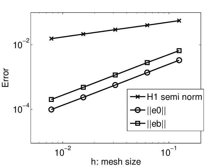
where . Notice that the diffusive coefficient vanishes at the origin. We set the exact solution to be . The configuration for the finite element partitions is the same as in test Case 1. We tested the weak Galerkin method on this problem, and the results are presented in Table 4 and Figure 1.
Since the diffusive coefficient is not uniformly positive definite on , we have no anticipation that the weak Galerkin approximation has any optimal rate of convergence, though the exact solution is smooth. It should be pointed out that the usual Lax-Milgram theorem is not applicable to such problems in order to have a result on the solution existence and uniqueness. However, one can prove that the discrete problem always has a unique solution when Gaussian quadratures are used in the numerical integration. Interestingly, the numerical experiments show that the weak Galerkin method converges with a rate of approximately in , in and . It is left for future research to explore a theoretical foundation of the observed convergence behavior.
| 1/8 | 5.61e-02 | 3.32e-03 | 6.60e-03 | 5.75e-02 | 5.48e-03 | 1.27e-02 |
|---|---|---|---|---|---|---|
| 1/16 | 4.03e-02 | 1.38e-03 | 2.81e-03 | 4.09e-02 | 2.59e-03 | 4.90e-03 |
| 1/32 | 2.95e-02 | 5.68e-04 | 1.16e-03 | 2.96e-02 | 1.23e-03 | 2.21e-03 |
| 1/64 | 2.15e-02 | 2.35e-04 | 4.83e-04 | 2.15e-02 | 5.97e-04 | 1.16e-03 |
| 1/128 | 1.55e-02 | 9.93e-05 | 2.02e-04 | 1.55e-02 | 2.91e-04 | 5.99e-04 |
| 0.4614 | 1.2687 | 1.2594 | 0.4697 | 1.0579 | 1.0912 |
4.3 Case 3: A Model Problem on a Domain with Corner Singularity
We consider the Laplace equation on a two-dimensional domain for which the exact solution possesses a corner singularity. For simplicity, we take and let the exact solution be given by
| (20) |
where and is a constant. Clearly, we have
where is any small, but positive number. Again, a uniform triangular mesh and the element are used in the numerical discretization. Note that the weak Galerkin for this problem is exactly the same as the standard mixed finite element method.
This model problem was numerically tested with and . The convergence rates are reported in Table 5 and Table 6. Notice that and behaves in a way as predicted by theory (5); i.e., they converge with rates given by and , respectively. The result also shows that the approximation on the element edge/face has a rate of convergence .
| 1/8 | 1.88e-01 | 6.40e-03 | 1.47e-02 | 2.54e-01 | 1.49e-02 | 4.30e-02 |
|---|---|---|---|---|---|---|
| 1/16 | 1.36e-01 | 2.20e-03 | 5.28e-03 | 1.84e-01 | 7.66e-03 | 3.01e-02 |
| 1/32 | 9.74e-02 | 7.62e-04 | 1.86e-03 | 1.32e-01 | 3.89e-03 | 2.12e-02 |
| 1/64 | 6.93e-02 | 2.65e-04 | 6.57e-04 | 9.42e-02 | 1.96e-03 | 1.49e-02 |
| 1/128 | 4.92e-02 | 9.33e-05 | 2.32e-04 | 6.69e-02 | 9.88e-04 | 1.05e-02 |
| 0.4852 | 1.5251 | 1.4992 | 0.4827 | 0.9805 | 0.5066 |
| 1/8 | 4.93e-01 | 1.69e-02 | 3.58e-02 | 6.65e-01 | 2.56e-02 | 1.25e-01 |
|---|---|---|---|---|---|---|
| 1/16 | 4.18e-01 | 7.07e-03 | 1.52e-02 | 5.66e-01 | 1.31e-02 | 1.05e-01 |
| 1/32 | 3.53e-01 | 2.94e-03 | 6.39e-03 | 4.79e-01 | 6.72e-03 | 8.85e-02 |
| 1/64 | 2.98e-01 | 1.22e-03 | 2.68e-03 | 4.04e-01 | 3.42e-03 | 7.44e-02 |
| 1/128 | 2.51e-01 | 5.14e-04 | 1.12e-03 | 3.40e-01 | 1.73e-03 | 6.25e-02 |
| 0.2437 | 1.2613 | 1.2489 | 0.2417 | 0.9717 | 0.2505 |
4.4 Case 4: A Model Problem with Intersecting Interfaces
This test problem is taken from [16], which has also been tested by other researchers [17, 20]. In two dimension, consider and the following problem
where in the first and third quadrants, and in the second and forth quadrants. Here is the identity matrix and , are two positive numbers. Consider an exact solution which takes the following form in polar coordinates:
where and
| (21) |
The parameters satisfy the following nonlinear relations
| (22) |
The solution is known to be in for any , and has a singularity near the origin .
One choice for the coefficients is to take , , , . We numerically solve this problem by using the weak Galerkin method with element on triangular meshes. It turns out that uniform triangular meshes are not good enough to handle the singularity in this problem. Indeed, we use a locally refined initial mesh, as shown in Figure 2, which consists of 268 triangles. This mesh is then uniformly refined, by dividing each triangle into 4 subtriangles, to get a sequence of nested meshes. Although this can not be compared with an adaptive mesh refinement process, it does improve the accuracy of the numerical approximation, as shown in our numerical results reported in Table 7. Since the mesh is not quasi-uniform, we do not expect that the theoretic error estimation (5) apply for this problem. An interesting observation of Table 7 is that, the norm appears to converge in a much faster rate than , while the opposite has usually been observed for other test cases. We believe that this is due to the use of a locally refined initial mesh in our testing process. When the actual value of reduces to the same level as the value of , its convergence rate slows down to the same as . Readers are also encouraged to derive their own conclusions from these numerical experiments.
We also observe that, when the initial mesh gets more refined near the origin, the convergence rates increase slightly. In Table 8, this trend is clearly shown. For each initial mesh, it is refined four times to get five levels of nested meshes. The convergence rates are computed based on these five nested meshes. The initial meshes are generated by refining only those triangles near the origin. Two examples of initial meshes are shown in Figure 2.


| level | ||||||
|---|---|---|---|---|---|---|
| 0 | 1.07e-01 | 3.97e-03 | 9.95e-03 | 1.47e-01 | 2.60e-02 | 1.97e-02 |
| 1 | 9.76e-02 | 2.92e-03 | 6.44e-03 | 1.26e-01 | 1.33e-02 | 1.94e-02 |
| 2 | 9.30e-02 | 2.51e-03 | 5.11e-03 | 1.16e-01 | 7.01e-03 | 1.91e-02 |
| 3 | 9.12e-02 | 2.21e-03 | 4.44e-03 | 1.11e-01 | 3.95e-03 | 1.88e-02 |
| 4 | 8.98e-02 | 1.95e-03 | 3.91e-03 | 1.07e-01 | 2.55e-03 | 1.84e-02 |
| 0.0604 | 0.2446 | 0.3229 | 0.1084 | 0.8461 | 0.0239 |
| # | Convergence rates , | |||||
|---|---|---|---|---|---|---|
| triangles | ||||||
| 268 | 0.0604 | 0.2446 | 0.3229 | 0.1084 | 0.8461 | 0.0239 |
| 300 | 0.0750 | 0.2623 | 0.3489 | 0.1206 | 0.8699 | 0.0373 |
| 332 | 0.0888 | 0.2818 | 0.3772 | 0.1329 | 0.8912 | 0.0487 |
| 364 | 0.1020 | 0.3031 | 0.4079 | 0.1454 | 0.9099 | 0.0586 |
| 396 | 0.1148 | 0.3266 | 0.4411 | 0.1581 | 0.9260 | 0.0673 |
| 428 | 0.1273 | 0.3522 | 0.4766 | 0.1711 | 0.9396 | 0.0749 |
| 460 | 0.1396 | 0.3802 | 0.5145 | 0.1843 | 0.9509 | 0.0817 |
| 492 | 0.1519 | 0.4105 | 0.5548 | 0.1978 | 0.9602 | 0.0878 |
| 524 | 0.1641 | 0.4432 | 0.5972 | 0.2117 | 0.9678 | 0.0932 |
4.5 Case 5: An Anisotropic Problem
Consider a two dimensional anisotropic problem defined in the square domain as follows
where the diffusive coefficient is given by
We chose a function and a Dirichlet boundary condition so that the exact solution is given by . In applying the weak Galerkin method, we use an anisotropic triangular mesh that was constructed by first dividing the domain into sub-rectangles, and then splitting each rectangle into two triangles by connecting a diagonal line. The characteristic mesh size is . We tested two cases with and . The results are reported in Tables 9 and 10. The tables show optimal rates of convergence for the weak Galerkin approximation in various metrics. The numerical experiment indicates that the weak Galerkin method can handle anisotropic problems and meshes without any trouble.
| 1/8 | 1.48e+0 | 1.95e-02 | 4.61e-02 | 2.70e+0 | 1.29e-01 | 4.13e-02 |
|---|---|---|---|---|---|---|
| 1/16 | 7.39e-01 | 5.11e-03 | 1.16e-02 | 1.35e+0 | 6.53e-02 | 1.06e-02 |
| 1/32 | 3.69e-01 | 1.29e-03 | 2.92e-03 | 6.80e-01 | 3.27e-02 | 2.67e-03 |
| 1/64 | 1.84e-01 | 3.24e-04 | 7.33e-04 | 3.40e-01 | 1.63e-02 | 6.68e-04 |
| 1/128 | 9.23e-02 | 8.12e-05 | 1.83e-04 | 1.70e-01 | 8.18e-03 | 1.66e-04 |
| 1.0010 | 1.9793 | 1.9942 | 0.9972 | 0.9975 | 1.9906 |
| 1/4 | 7.98e+0 | 6.80e-02 | 2.93e-01 | 1.58e+1 | 2.52e-01 | 1.49e-01 |
|---|---|---|---|---|---|---|
| 1/8 | 3.89e+0 | 2.07e-02 | 7.44e-02 | 8.18e+0 | 1.30e-01 | 4.22e-02 |
| 1/16 | 1.91e+0 | 5.43e-03 | 1.88e-02 | 4.12e+0 | 6.53e-02 | 1.09e-02 |
| 1/32 | 9.54e-01 | 1.37e-03 | 4.72e-03 | 2.06e+0 | 3.27e-02 | 2.74e-03 |
| 1/64 | 4.76e-01 | 3.44e-04 | 1.18e-03 | 1.03e+0 | 1.63e-02 | 6.84e-04 |
| 1.0161 | 1.9160 | 1.9897 | 0.9857 | 0.9883 | 1.9492 |
4.6 Case 6: A Three-Dimensional Model Problem
The final test problem is a three dimensional Laplace equation defined on , with a Dirichlet boundary condition and an exact solution given by . The purpose of this test problem is to examine the convergence rate of the cubic element. The results are reported in Table 11.
In addition to the optimal rates of convergence as shown in Table 11, on can also see a superconvergence for . The same result is anticipated for 2D rectangular elements. It is left to interested readers for a further investigation, especially for model problems with variable coefficients.
| 1/8 | 1.85e-01 | 1.62e-02 | 4.27e-02 | 1.22e+00 | 1.34e-01 | 3.63e-02 |
|---|---|---|---|---|---|---|
| 1/12 | 8.53e-02 | 7.69e-03 | 1.94e-02 | 8.19e-01 | 9.14e-02 | 1.96e-02 |
| 1/16 | 4.86e-02 | 4.42e-03 | 1.10e-02 | 6.15e-01 | 6.89e-02 | 1.18e-02 |
| 1/20 | 3.13e-02 | 2.85e-03 | 7.07e-03 | 4.92e-01 | 5.52e-02 | 7.78e-03 |
| 1.9389 | 1.8984 | 1.9618 | 0.9914 | 0.9737 | 1.6779 |
References
- [1] R.A. Adams and J.J.F. Fournier, Sobolev Spaces, Academic Press, 2nd ed., 2003.
- [2] D. Arnold, F. Brezzi, B. Cockburn, and D. Marini, Unified analysis of discontinuous Galerkin methods for elliptic problems, SIAM J. Numer. Anal., 39(2002), pp. 1749–1779.
- [3] C. Bahriawati and C. Carstensen, Three Matlab implementations of the lowest order Raviart-Thomas MFEM with a posteriori error control, Comp. Meth. Appl. Math., 5(2005), pp. 333–361.
- [4] C.E. Baumann and J.T. Oden, A discontinuous hp finite element method for convection-diffusion problems, Comput. Meth. Appl. Mech. Engrg., 175(1999), pp. 311–341.
- [5] F. Brezzi, J. Douglas, and L. Marini, Two families of mixed finite elements for second order elliptic problems, Numer. Math., 47(1985), pp. 217–235.
- [6] C. Bernardi and R. Verfürth, Adaptive finite element methods for elliptic equations with non-smooth coefficients, Numer. Math., 85(2000), pp. 579–608.
- [7] S.C. Brenner, L. Owens, and L.Y. Sung, A weakly over-penalized symmetric interior penalty method, Electronic Transactions on Numerical Analysis (ETNA), 30(2008), pp. 107–127.
- [8] S.C. Brenner and L.R. Scott, The mathematical theory of finite element methods, Springer, 3rd ed., 2008.
- [9] F. Brezzi and M. Fortin, Mixed and hybrid finite element methods, Springer-Verlag, 1991.
- [10] P.G. Ciarlet, The finite element method for elliptic problems, North-Holland, Amsterdam, 1978.
- [11] B. Cockburn, J. Gopalakrishnan, and R. Lazarov, Unified hybridization of discontinuous Galerkin, mixed, and continuous Galerkin methods for second order elliptic problems, SIAM J. Numer. Anal., 47(2009), pp. 1319–1365.
- [12] B. Cockburn, G.E. Karniadakis, and C.-W. Shu, Discontinuous Galerkin Methods: Theory, Computation and Applications, Lect. Notes Comput. Sci. Engrg. 11, Springer-Verlag, New York, 2000.
- [13] M. Crouzeix and P. Raviart, Conforming and nonconforming finite element methods for solving the stationary Stokes equations, RAIRO, Anal. Numer. 3(1973), pp. 33–75.
- [14] Y. Epshteyn and B. Riviere, Estimation of penalty parameters for symmetric interior penalty Galerkin methods, J. Comput. Appl. Math., 206(2007), pp. 843–872.
- [15] C. Johnson, Numerical solution of partial differential equations by the finite element method, Dover, 2009.
- [16] R.B. Kellog, On the Poisson equation with intersecting interfaces, Appl. Anal., 4(1976), pp. 101–129.
- [17] J. Liu, L. Mu, and X. Ye, Convergence of the discontinuous finite volume method for elliptic problems with minimal regularity, Preprint submitted to J. Comput. Appl. Math, (2011).
- [18] J. Liu and M. Yang, A weakly over-penalized finite volume element method for elliptic problems, Preprint submitted to Numer. Meth. PDEs, (2011).
- [19] S.D. Margenov and P.S. Vassilevski, Algebraic multilevel preconditioning of anisotropic elliptic problems, SIAM J. Sci. Comput., 15(1994), pp. 1026–1037.
- [20] P. Morin, R.H. Nochetto, and K.G. Siebert, Convergence of adaptive finite element methods, SIAM Rev., 44(2002), pp. 631–658.
- [21] P. Raviart and J. Thomas, A mixed finite element method for second order elliptic problems, Mathematical Aspects of the Finite Element Method, I. Galligani, E. Magenes, eds., Lectures Notes in Math. 606, Springer-Verlag, New York, 1977.
- [22] S. Sun, Discontinuous Galerkin methods for reactive transport in porous media, Ph.D. dissertation, The University of Texas at Austin, 2003.
- [23] J. Wang and X. Ye, A weak Galerkin finite element method for second-order elliptic problems, arXiv:1104.2897v1 [math.NA].
- [24] J. Wang and X. Ye, A weak Galerkin finite element method for Stokes problems, Preprint, 2011.
- [25] B. Riviére, M.F. Wheeler, and V. Girault, A priori error estimates for finite element methods based on discontinuous approximation spaces for elliptic problems, SIAM J. Numer. Anal., 39(2001), pp. 902–931.
- [26] T.P. Wihler and B. Riviére, Discontinuous Galerkin methods for second-order elliptic PDE with low-regularity solutions, J. Sci. Comput., 46(2011), pp. 151–165.