Identifying Non-Resonant Kepler Planetary Systems

Identifying Non-Resonant Kepler Planetary Systems–References2011

Dimitri Veras ^†^†thanks: E-mail:veras@ast.cam.ac.uk Affiliation: Institute of Astronomy, University of Cambridge, Madingley Road, Cambridge CB3 0HA, UK Eric B. Ford Affiliation: Astronomy Department, University of Florida, 211 Bryant Space Sciences Center, Gainesville, Florida 32111, USA

Accepted 2011 November 01. Received 2011 October 26; in original form 2011 October 09

Abstract

The Kepler mission has discovered a plethora of multiple transiting planet candidate exosystems, many of which feature putative pairs of planets near mean motion resonance commensurabilities. Identifying potentially resonant systems could help guide future observations and enhance our understanding of planetary formation scenarios. We develop and apply an algebraic method to determine which Kepler 2-planet systems cannot be in a 1st-4th order resonance, given the current, publicly available data. This method identifies when any potentially resonant angle of a system must circulate. We identify and list 70 near-resonant systems which cannot actually reside in resonance, assuming a widely-used formulation for deriving planetary masses from their observed radii and that these systems do not contain unseen bodies that affect the interactions of the observed planets. This work strengthens the argument that a high fraction of exoplanetary systems may be near resonance but not actually in resonance.

Keywords:

planets and satellites: dynamical evolution and stability, celestial mechanics

1 Introduction

The Kepler mission has identified more planetary candidates than the total number of extrasolar planets that were known before its launch (Borucki et al., 2011). This windfall of mission results enables investigators to perform better statistical analyses to more accurately estimate properties of the exoplanet population. A dynamical question of particular interest is, “what is the frequency of resonant extrasolar systems?”

The absence of resonance may be just as important, especially in systems with tightly packed but stable configurations (Lissauer et al., 2011a) and/or which might feature transit timing variations that span several orders of magnitude (Ford et al., 2011; Veras et al., 2011). Resonances may be a signature of a particular mode of planetary formation; they are likely to be indicative of convergent migration in nascent protoplanetary disks (Thommes & Lissauer, 2003; Kley et al., 2004; Papaloizou & Szuszkiewicz, 2005). Their absence might be indicative of a dynamical history dominated by gravitational planet-planet scattering (Raymond et al., 2008). Alternatively, resonant statistics might best constrain how disk evolution and gravitational scattering interface (Matsumura et al., 2010; Moeckel & Armitage, 2011).

Lissauer et al. (2011b) provide a comprehensive accounting of all planetary period ratios in Kepler systems, and present distributions and statistics linking the periods to potentially resonant behavior. Our focus here simply is to identify which systems cannot be resonant. A variety of mean motion resonances are known to exist in the Solar System and extrasolar systems. However, for most of these cases, the masses, eccentricities and longitude of pericenters have been measured directly. Contrastingly, for Kepler systems, these parameters are constrained poorly, if at all. Hence, analyzing resonant Kepler systems poses a unique challenge.

In order to address this situation, we present an analysis that i) treats the entire potential eccentricity phase space in most cases, ii) considers a relevant limiting case of the unknown orbital angles, and iii) pinpoints the manner in which planetary masses can affect the possibility of resonance. The analysis is also entirely algebraic, allowing us to avoid numerical integrations and hence investigate an ensemble of systems. The results produce definitive claims about which systems cannot be in resonance, given the current data. We consider the ensemble of Kepler two-planet systems which may be near 1st-4th order eccentricity-based resonances, under the assumptions of coplanarity, non-crossing orbits, and the nonexistence of additional, as-yet-unidentified planets that would affect the interactions of the observed planets. In Section 2, we explain our analytical model, and then apply it in Section 3. We present our list of non-resonant Kepler systems in Table 1, and briefly discuss and summarize our results in Section 4.

2 Analytic Model

2.1 Proving Circulation

The behavior of linear combinations of orbital angles from each of the two planets determines if a system is in resonance or not. “Libration” is a term often used to denote oscillation of a resonant angle, and “circulation” often refers to the absence of oscillation. Resonant systems must have a librating angle; for mean motion resonances, the focus of this study, the librating angle incorporates the positions of both planets. This seemingly simple criterion, however, belies complex behavior often seen in real systems.

For example, Brasser et al. (2004) illustrate how the resonant angle of a Neptunian Trojan can switch irregularly between libration and circulation, while Farmer & Goldreich (2006) illustrate how long periods of circulation can be punctuated by short periods of libration. Characterizing libration versus circulation in extrasolar systems – often with two massive extrasolar planets – sometimes necessitates careful statistical measures (Veras & Ford, 2010).

The gravitational potential between two coplanar bodies orbiting a star can be described by two “disturbing functions,” denoted by $R_{w}$ , with $w=1,2$ , which are infinite linear sums of cosine terms with arguments of the form

\phi(t)=j_{1}\lambda_{1}(t)+j_{2}\lambda_{2}(t)+j_{3}\varpi_{1}(t)+j_{4}\varpi_{2}(t),

(1)

where $\lambda$ represents mean longitude, $\varpi$ represents longitude of pericenter, the “ $j$ ” values represent integer constants, and the subscript “ $1$ ” refers to the outer body while the subscript “ $2$ ” refers to the inner body. We choose this subscripting convention so our equations conform with those in Murray & Dermott (1999) and Veras (2007). The mean longitude is directly proportional to mean longitude at epoch, denoted by $\epsilon_{w}$ , such that $\lambda_{w}\equiv\varpi_{w}+M_{w}=\pi_{w}+\Omega_{w}+M_{w_{0}}+\int_{t_{0}}^{t}n_{w}(t^{\prime})dt^{\prime}=\epsilon_{w}+\int_{t_{0}}^{t}\mu_{w}^{(1/2)}a_{w}(t^{\prime})^{(-3/2)}dt^{\prime}$ , where $M_{w}$ denotes mean anomaly, $\pi_{w}$ denotes argument of pericenter, and $n_{w}$ denotes mean motion. The mean motion is related to its semimajor axis, $a_{w}$ , and mass through Kepler’s third law by $n_{w}^{2}a_{w}^{3}=\mu_{w}$ , where $\mu_{w}=G\left(m_{0}+m_{w}\right)$ , with $m_{w}$ representing the planet’s mass, $m_{0}$ the central body’s mass, and $G$ the universal gravitational constant.

The time derivative of Equation (1) yields:

	$\displaystyle\dot{\phi}(t)$	$\displaystyle=$	$\displaystyle j_{1}\mu_{1}^{\frac{1}{2}}a_{1}^{-\frac{3}{2}}(t)+j_{1}\dot{\epsilon}_{1}(t)+j_{2}\mu_{2}^{\frac{1}{2}}a_{2}^{-\frac{3}{2}}(t)+j_{2}\dot{\epsilon}_{2}(t)$		(2)
		$\displaystyle+$	$\displaystyle j_{3}\dot{\varpi}_{1}(t)+j_{4}\dot{\varpi}_{2}(t).$		(2)

Lagrange’s Planetary Equations (e.g., Murray & Dermott, 1999, pp. 251-252) relevant to Eq. (2) are:

	$\displaystyle\frac{d\epsilon_{w}}{dt}$	$\displaystyle=$	$\displaystyle-a_{w}^{\frac{1}{2}}A_{w,1}\frac{\partial R_{w}}{\partial a_{w}}+a_{w}^{-\frac{1}{2}}A_{w,2}A_{w,3}\frac{\partial R_{w}}{\partial e_{w}},$		(3)
	$\displaystyle\frac{d\varpi_{w}}{dt}$	$\displaystyle=$	$\displaystyle a_{w}^{-\frac{1}{2}}A_{w,2}\frac{\partial R_{w}}{\partial e_{w}},$		(4)

where

$\displaystyle A_{w,1}$	$\displaystyle=$	$\displaystyle 2\mu_{w}^{-\frac{1}{2}},$	(5)
$\displaystyle A_{w,2}$	$\displaystyle=$	$\displaystyle\mu_{w}^{-\frac{1}{2}}e_{w}^{-1}{\left(1-e_{w}^{2}\right)}^{\frac{1}{2}},$	(6)
$\displaystyle A_{w,3}$	$\displaystyle=$	$\displaystyle 1-{\left(1-e_{w}^{2}\right)}^{\frac{1}{2}}.$	(7)

The form of $R_{w}$ used dictates how to proceed. Veras (2007) expresses Ellis & Murray’s (2000) disturbing function as

R_{w}=a_{1}^{-1}\sum_{y=1}^{\infty}\left[\sum_{p=1}^{\infty}C_{w}^{(y,p)}X^{(y,p)}\right]\cos{\phi^{(y)}},

(8)

where $C_{w}^{(i,p)}$ is a function of the masses and semimajor axes, and $X^{(y,p)}$ is a function of the eccentricities and inclinations. Both of these auxiliary variables contain the detailed functional forms needed to model individual resonances.

When inserted into Eqs. (2)-(4), the disturbing function will yield:

\dot{\phi}^{(u)}=\sum_{y}\left(D^{(y,u)}\cos{\phi^{(y)}}\right)+E^{(u)},

(9)

where $\dot{\phi}^{(u)}$ is a potentially resonant angle, $D^{(y,u)}$ is an explicit algebraic function of the masses and orbital elements, and

E^{(u)}=\sum_{w=1}^{2}j_{w}^{(u)}\mu_{w}^{\frac{1}{2}}a_{w}^{-\frac{3}{2}}.

(10)

Hence, a particular angle $\phi^{(u)}$ cannot librate if

\sum|D^{(y,u)}|<|E^{(u)}|.

(11)

Equation (11) represents the criterion for an angle to circulate. Note that no integrations are required to evaluate the criterion. For systems which cannot be in resonance, the maximum value of $\sum|D^{(y,u)}|/|E^{(u)}|\equiv\beta_{u}$ provides an estimate of the proximity to a potential resonance.

The dependence these variables have on planetary mass is important to understand for the implications for Kepler systems: $\mu_{1}$ or $\mu_{2}$ appears in each of the terms in $E^{(u)}$ and $D^{(y,u)}$ , and are insensitive to the planetary masses, as long as these masses are negligible compared to the star’s mass. Further, each term in $D^{(y,u)}$ is linearly proportional to either $m_{1}$ or $m_{2}$ . Therefore, if $m_{1}$ and $m_{2}$ are both scaled by the same factor of their radii in a common mass-radius relationship, then the relative strength of the terms in $D^{(y,u)}$ will vary by a factor proportional to the planetary radii ratio. The signs of these terms depend on the resonance being studied. Hence, for a particular resonance, one may determine which terms are additive, and obtain an explicit dependence on planetary mass.

2.2 Hill Stability

Unless two bodies are resonantly locked in a configuration that allows for crossing orbits (such as Neptune and Pluto), the bodies will undergo dynamical instability if their eccentricities are too great and their semimajor axis difference is too small. Planets whose orbits never cross are said to be Hill stable, and obey (Gladman, 1993):

	$\displaystyle\frac{1+\eta_{1}+\eta_{2}}{{\left(\eta_{1}+\eta_{1}\eta_{2}+\eta_{2}\right)^{3}}}\left[\eta_{1}+\frac{\eta_{2}}{\alpha}\right]$	(12)
$\displaystyle\times$	$\displaystyle\left[\eta_{2}\sqrt{\alpha\left(1-e_{2}^{2}\right)}+\eta_{1}\sqrt{1-e_{1}^{2}}\right]^{2}>$
	$\displaystyle 1+\frac{3^{\frac{4}{3}}\eta_{1}\eta_{2}}{\left(\eta_{1}+\eta_{2}\right)^{\frac{4}{3}}}-\frac{\eta_{1}\eta_{2}\left(11\eta_{2}+7\eta_{1}\right)}{3\left(\eta_{1}+\eta_{2}\right)^{2}},$

where $\eta_{1}\equiv m_{1}/m_{0}$ , $\eta_{2}\equiv m_{2}/m_{0}$ , and $\alpha=a_{2}/a_{1}$ . In principle, systems which do not satisfy Eq. (12) may be stable, but generally this is true only for resonant systems. Thus, we focus our efforts only on those systems which are provably stable. Fig. 1 displays level curves of Eq. (12) for different values of $\eta_{1}$ and $\eta_{2}$ ( $10^{-3}m_{\odot}$ -solid, $10^{-4}m_{\odot}$ -dotted, $10^{-5}m_{\odot}$ -dashed, $10^{-6}m_{\odot}$ -dashed-dot) and at different commensurabilities of interest ( $7$ : $6$ -magenta, $3$ : $2$ -green, $5$ : $3$ -red, $2$ : $1$ -blue, $3$ : $1$ -salmon), which each correspond to the appropriate value of $\alpha$ . The range of eccentricities plotted and considered in this study is well within the absolute convergence limits of this disturbing function (Ferraz-Mello, 1994; Sidlichovsky & Nesvorny, 1994) and corresponds roughly to a regime where a fourth-order treatment (as in Veras 2007) is accurate to within $\approx 0.3^{4}<1\%$ .

Refer to caption — Figure 1: Hill stability eccentricity portrait. Each curve (for the following planet/star mass ratios: solid lines - $10^{-3}m_{\odot}$ ; dotted lines - $10^{-4}m_{\odot}$ ; dashed lines - $10^{-5}m_{\odot}$ ; dot-dashed lines - $10^{-6}m_{\odot}$ ) bounds eccentricities at which two planets may be Hill stable, for semimajor axes ratios corresponding to the following commensurabilities (in order of dashed lines going outward from the origin): $7$ : $6$ -magenta, $3$ : $2$ -green, $5$ : $3$ -red, $2$ : $1$ -blue, and $3$ : $1$ -salmon. Stable systems lie below the curves, and observed Kepler systems are assumed to be stable. Note that the curves are not symmetrical about the origin. The solid salmon curve indicates that nearly all planets whose semimajor axis ratio is within a factor of $\approx 2$ are subject to stability constraints for $e_{1},e_{2}<0.3$ .

3 Application to Kepler Systems

3.1 Method

We use the publicly available Kepler database¹¹ 1 at http://archive.stsci.edu/kepler/planet_candidates.html, which provides directly measured values for planetary periods and estimated values of the stellar mass. With these, we estimate the planetary semimajor axes by assuming values for the planetary masses based on a mass-radius relationship. Lissauer et al. (2011b) estimate these values using:

m_{1}=\left(\frac{R_{1}}{R_{\oplus}}\right)^{b}m_{\oplus}

(13)

where $b=2.06$ . A similar formula holds for the other planet in the system.

We assume Eq. (13) to be true, and then determine the “nearness” of all two-planet systems to a mean motion commensurability through

\left(1-x/100\right)\left(j_{1}/j_{2}\right)^{2/3}<a_{1}/a_{2}<\left(1+x/100\right)\left(j_{1}/j_{2}\right)^{2/3},

(14)

where $x$ effectively measures the percent offset from resonance in semimajor axis space. Because we consider all potential resonances up to fourth-order, the same planetary system may be close to several resonances. We refer to a “near-resonant instance” as a case where Eq. (14) is satisfied. We plot the cumulative frequency of near-resonant instances as a function of $x$ in Fig. 2. Not included in the figure are $(j_{1},j_{2})$ multiplicities: higher-order harmonic angles which can be expressed as a linear combination of the angles with the lowest-order relatively prime values of $j_{1}$ and $j_{2}$ , although these higher-order terms are included in the computation of $D^{(y,u)}$ (Veras, 2007, see, e.g. Table 4 of). The figure demonstrates the potentially wide variety of resonant configurations which may be possible depending on one’s definition of “near-resonant”. We choose to be conservative and include all “near-resonant instances” on the plots in our analysis.

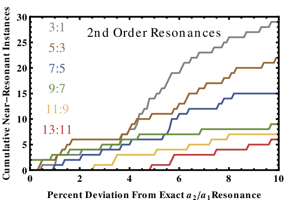
Having identified a potential resonance with a given $j_{1}$ and $j_{2}$ , and having adopted $m_{1}$ , $m_{2}$ , $a_{1}$ and $a_{2}$ , we then sample the entire eccentricity phase space for which the planets are Hill stable. In the few cases where Hill stable systems admit $e_{1}>0.3$ and/or $e_{2}>0.3$ , we limit the eccentricities to these values for accuracy and convergence considerations, as described earlier. At each of 31 evenly-spaced values of $e_{2}$ from $0$ to $0.3$ , we compute the maximum Hill stable value of $e_{1}$ , and then sample 31 evenly-spaced values of $e_{1}$ from 0 to that Hill maximum value. Finally, we compute $\beta_{u}=\sum_{y}|D^{(y,u)}|/|E^{(u)}|$ for every possible disturbing function argument for $j_{1},|j_{2}|>0$ which satisfy the d’Alembert relations²² 2 The secular arguments $j_{1}=j_{2}=0$ up to 4th-order are included in the computation of $D^{(y,u)}$ even though we test only for circulation of angles which can lead to mean motion resonance.. If no value of $\beta_{u}$ exceeds unity, then we flag the system as non-resonant and record the highest value of $\beta_{u}$ as a proxy for closest proximity to resonance.

3.2 Results

Of the 116 Kepler systems with two transiting candidates for which public data is available, 94 have planets with periods similar enough to each other to be considered “near-resonant” for at least one 1st-4th order resonance with $x\leq 10$ . These 94 systems registered a total of 465 near-resonant instances for $j_{1}<20$ . Of those 465, 313 cannot be resonant. Only 4 systems (KOI #s: 89, 523, 657, 738) have planets which may be resonant for at least one instance and cannot be resonant for at least one other, thereby restricting the system’s potential membership in some resonances. For 20 systems (KOI #s: 82, 111, 115, 124, 222, 271, 314, 341, 543, 749, 787, 841, 870, 877, 945, 1102, 1198, 1221, 1241, 1589), mean motion resonance could not be ruled out for any of the near-resonant instances sampled. Quantifying the likelihood of resonance in these systems would require future detailed individual analysis.

We claim that the remaining 70 systems cannot be in resonance, despite their close proximity to a commensurability. We list these systems in Table 1, along with the number of their near-resonant instances, their maximum value of $\beta$ and the mean motion resonance this value corresponds to. The larger the value of $\beta$ , the closer the system is to having parameters which could admit resonance. In most cases, $\beta<0.5$ , meaning that the systems are well outside of resonance. Notable exceptions are KOI 244, KOI 431, KOI 508, KOI 775, and KOI 1396, three of which are close to the strong $2$ : $1$ commensurability. KOI 1151 is so close to so many commensurabilities because for that system, $1/\alpha=1.26$ , meaning that the planets are tightly packed and on the edge of stability.

Table 1: Non-Resonant 2-Planet Kepler Systems.

KOI	Number of	Closest	Maximum
Number	Near-Res Instances	$j_{1}$ : $\|j_{2}\|$	$\beta$
116	1	$3$ : $1$	0.078
123	1	$3$ : $1$	0.018
150	1	$3$ : $1$	0.027
153	4	$9$ : $5$	0.28
209	2	$3$ : $1$	0.22
220	6	$9$ : $5$	0.039
232	3	$7$ : $3$	0.016
244	3	$2$ : $1$	0.67
270	3	$3$ : $1$	0.0043
279	4	$9$ : $5$	0.17
282	1	$3$ : $1$	0.016
284	2	$3$ : $1$	0.033
291	1	$4$ : $1$	0.010
313	3	$7$ : $3$	0.043
339	1	$3$ : $1$	0.0043
343	2	$7$ : $3$	0.12
386	2	$5$ : $2$	0.16
401	1	$5$ : $1$	0.031
416	1	$5$ : $1$	0.024
431	2	$5$ : $2$	0.60
440	1	$3$ : $1$	0.040
446	6	$9$ : $5$	0.18
448	2	$4$ : $1$	0.038
456	1	$3$ : $1$	0.048
459	2	$3$ : $1$	0.042
474	3	$5$ : $2$	0.020
475	4	$9$ : $5$	0.23
497	1	$3$ : $1$	0.31
508	2	$2$ : $1$	0.84
509	2	$3$ : $1$	0.042
510	3	$7$ : $3$	0.035
518	1	$3$ : $1$	0.028
534	2	$7$ : $3$	0.37
551	3	$2$ : $1$	0.25
573	1	$3$ : $1$	0.11
584	2	$2$ : $1$	0.083
590	2	$4$ : $1$	0.0049
612	3	$7$ : $3$	0.21
638	2	$3$ : $1$	0.12
645	2	$3$ : $1$	0.031
658	6	$9$ : $5$	0.10
672	3	$5$ : $2$	0.12
676	1	$3$ : $1$	0.12
691	5	$9$ : $5$	0.11
693	5	$9$ : $5$	0.17
700	1	$3$ : $1$	0.027
708	3	$7$ : $3$	0.036
736	2	$3$ : $1$	0.063
752	1	$5$ : $1$	0.0049
775	2	$2$ : $1$	0.78
800	3	$3$ : $1$	0.023
837	3	$9$ : $5$	0.035
842	2	$3$ : $1$	0.090
853	6	$9$ : $5$	0.19
869	1	$5$ : $1$	0.051
896	3	$5$ : $2$	0.14
954	2	$5$ : $1$	0.0059
1015	2	$7$ : $3$	0.085
1060	2	$5$ : $2$	0.028
1113	1	$3$ : $1$	0.030
1151	15	$9$ : $7$	0.044
1163	2	$3$ : $1$	0.015

Table 2: …Table 1 continued

KOI	Number of	Closest	Maximum
Number	Near-Res Instances	$j_{1}$ : $\|j_{2}\|$	$\beta$
1203	3	$7$ : $3$	0.059
1215	4	$9$ : $5$	0.084
1278	1	$4$ : $1$	0.0081
1301	1	$3$ : $1$	0.13
1307	3	$7$ : $3$	0.049
1360	2	$5$ : $2$	0.27
1364	1	$3$ : $1$	0.19
1396	6	$9$ : $5$	0.89

We don’t expect variations in the masses of the Kepler planets to greatly affect the composition of Table 1, assuming that the value of $b$ from Eq. (13) does not vary by more than a few tenths from 2.06. The value of $\beta$ for a particular system can hint at the potential implications of mass variation. In particular, values of $\beta$ close to unity indicate that the system is on the border of potentially resonant behavior. For example, for KOI 1396 ( $\beta=0.89$ ), if we set $b=1.7$ , then the resulting planetary masses could allow the system to harbor a (weak) $9$ : $5$ resonance.

4 Conclusion and Implications

We have identified 70 Kepler 2-planet near-commensurate systems which cannot be in an eccentricity-based mean motion resonance of up to 4th-order. These systems, may, in principle, achieve resonance with crossing orbits or high ( $e>0.3$ ) eccentricities that could remain stable. The criterion of Eq. (11) is generally applicable to any 3-body system suspected of harboring resonant behavior. We caution that these results could be affected by the presence of additional planets which have yet to be detected.

Systems which are provably non-resonant may be incorporated in formation studies and detailed analyses of Kepler data. Kepler multi-planet systems may be preferentially clustered around particular resonances (Lissauer et al., 2011b). One possible explanation may be that convergent migration locks planets in a mean motion resonance which later gets broken by some additional perturbation. We find that Kepler multi-planet systems preferentially cluster around commensurabilities where $|j_{2}|$ is low and rarely do so when $|j_{2}|$ is high. In particular, the number of Kepler systems near the $2$ : $1$ , $3$ : $2$ , $3$ : $1$ and $5$ : $3$ commensurabilities is higher than what would be expected from a random distribution of Kepler planet candidate semimajor axes. Provably non-resonant planets may also complement transit timing variation statistics, as these variations take on distinctly different characteristics for near-resonant and resonant systems (Veras et al., 2011).

The analysis in this work cannot be performed with Kepler systems that contain more than 2 planet candidates because i) more disturbing functions must be incorporated, and hence the criteria for circulation becomes decidedly more complex, and ii) analytical formulae for Hill stability no longer hold. Figure 29 of Chatterjee et al. (2008) demonstrate that widely-separated pairs of planets in 3-planet systems whose orbits would be Hill stable in the 2-planet-only case may eventually become unstable. Even if a multi-planet system was assumed to be stable over a specified period of time and more disturbing functions were introduced, the resulting expansion of the phase space might render the computational cost of a similar algebraic analysis prohibitive compared to numerical integrations. However, the investigation of the nonplanar 2-planet case with inclination-based resonances might be a fruitful avenue to explore, especially because multiple transits detected by Kepler may constrain the planets’ mutual inclination, albeit weakly.

Acknowledgments

We thank an anonymous referee, Geoff Marcy, and Darin Ragozzine for valuable comments. This material is based on work supported by the National Aeronautics and Space Administration under grant NNX08AR04G issued through the Kepler Participating Scientist Program.

References

Borucki et al. (2011) Borucki, W. J., Koch, D. G., Basri, G., et al. 2011, ApJ, 736, 19
Brasser et al. (2004) Brasser, R., Heggie, D. C., & Mikkola, S. 2004, Celestial Mechanics and Dynamical Astronomy, 88, 123
Chatterjee et al. (2008) Chatterjee, S., Ford, E. B., Matsumura, S., & Rasio, F. A. 2008, ApJ, 686, 580
Ellis & Murray (2000) Ellis, K. M., & Murray, C. D. 2000, Icarus, 147, 129
Farmer & Goldreich (2006) Farmer, A. J., & Goldreich, P. 2006, Icarus, 180, 403
Ferraz-Mello (1994) Ferraz-Mello, S. 1994, Celestial Mechanics and Dynamical Astronomy, 58, 37
Ford et al. (2011) Ford, E. B., Rowe, J. F., Fabrycky, D. C., et al. 2011, ApJS, 197, 2
Gladman (1993) Gladman, B. 1993, Icarus, 106, 247
Kley et al. (2004) Kley, W., Peitz, J., & Bryden, G. 2004, A&A, 414, 735
Lissauer et al. (2011a) Lissauer, J. J., Fabrycky, D. C., Ford, E. B., et al. 2011a, Nature, 470, 53
Lissauer et al. (2011b) Lissauer, J. J., Ragozzine, D., Fabrycky, D. C., et al. 2011b, arXiv:1102.0543
Matsumura et al. (2010) Matsumura, S., Thommes, E. W., Chatterjee, S., & Rasio, F. A. 2010, ApJ, 714, 194
Moeckel & Armitage (2011) Moeckel, N., & Armitage, P. J. 2011, arXiv:1108.5382
Murray & Dermott (1999) Murray, C. D., & Dermott, S. F. 1999, Solar system dynamics by Murray, C. D., 1999,
Papaloizou & Szuszkiewicz (2005) Papaloizou, J. C. B., & Szuszkiewicz, E. 2005, MNRAS, 363, 153
Raymond et al. (2008) Raymond, S. N., Barnes, R., Armitage, P. J., & Gorelick, N. 2008, ApJL, 687, L107
Sidlichovsky & Nesvorny (1994) Sidlichovsky, M., & Nesvorny, D. 1994, A&A, 289, 972
Thommes & Lissauer (2003) Thommes, E. W., & Lissauer, J. J. 2003, ApJ, 597, 566
Veras (2007) Veras, D. 2007, Celestial Mechanics and Dynamical Astronomy, 99, 197
Veras & Ford (2010) Veras, D., & Ford, E. B. 2010, ApJ, 715, 803
Veras et al. (2011) Veras, D., Ford, E. B., & Payne, M. J. 2011, ApJ, 727, 74