Cosmological dynamics of fourth order gravity: A compact view
Abstract
We construct a compact phase space for flat FLRW spacetimes with standard matter described by a perfect fluid with a barotropic equation of state for general theories of gravity, subject to certain conditions on the function . We then use this framework to study the behaviour of the phase space of Universes with a non-negative Ricci scalar in gravity. We find a number of interesting cosmological evolutions which include the possibility of an initial unstable power-law inflationary point, followed by a curvature fluid dominated phase mimicking standard radiation, then passing through a standard matter (CDM) era and ultimately evolving asymptotically towards a de-Sitter-like late-time accelerated phase.
pacs
98.80.CqI Introduction
The CDM (or Concordance) Model [1] is one of the greatest successes of General Relativity. It reproduces beautifully all the main observational results e.g., the dimming of type Ia Supernovae [2], Cosmic Microwave Background Radiation (CMBR) anisotropies [3], Large Scale Structure formation [4], baryon oscillations [5] and weak lensing [6]). Unfortunately, this model is also affected by significant fine-tuning problems related to the vacuum energy scale and this has led to a considerable amount of effort throughly exploring other viable theoretical schemes.
Currently, one of the most popular alternatives to the CDM model is based on gravitational actions which are non-linear in the Ricci curvature and/or contain terms involving combinations of derivatives of : the so called theories of gravity [9, 10, 11, 12]. Such models first became popular in the 1980’s because it was shown that they can be derived from fundamental physical theories (Like M-theory) and naturally admit a phase of accelerated expansion, which could be associated with an early universe inflationary phase [8]. The fact that the phenomenology of Dark Energy requires the presence of a similar phase (although only a late time - low energy one) has recently revived interest in these models. In particular, the idea that Dark Energy may have a geometrical origin, i.e., that there is a connection between Dark Energy and a non-standard behavior of gravitation on cosmological scales is now a very active area of research (see for example [13, 14, 15, 16, 17, 18, 15, 19]).
Unfortunately efforts to obtain an understanding of the physics of these theories are hampered by the complexity of the fourth-order field equations, making it difficult to obtain both exact and numerical solutions, which can be compared with observations. Recently however, progress has been made in resolving these issues using a number of useful techniques. One such method, based on the theory of dynamical systems [20] has proven to be very successful in providing a simple way of obtaining exact solutions and a (qualitative) description of the global dynamics of these models [22]. The dynamical systems analysis has up to now approached this problem in the conventional way, by first exploring the finite equilibrium points and then computing the asymptotic behavior of the phase-space using the classical method of Poincare projections.
In this paper we develop an alternative scheme which involves compactifying the phase space for general theories of gravity, subject to certain conditions on the function . We then use this framework to study the behaviour of the phase space of Universes with a non-negative Ricci scalar in gravity. We find a number of interesting cosmological evolutions, which include the possibility, at least in principle, where the Universe begins close to at an unstable power-law inflationary equilibrium point, then evolves towards a curvature fluid dominated phase where the effective equation of state mimics standard radiation with (we will refer to such phases as radiation-like), then passes through a standard matter (CDM) era and ultimately evolves asymptotically towards a de-Sitter-like late-time accelerated phase.
We also show that as , all the fixed points that approach the CDM subspace of the complete state space of gravity, are unstable. This implies that the behavior of the solutions of a fourth order theory which is close to CDM may be completely different from those of CDM and one needs to do a careful analysis of the solutions rather than a priori assuming any global behavior of the trajectories.
II The field equations for fourth order gravity
The natural extension of standard General Relativity is to consider a Lagrangian that contains curvature invariants of higher than linear order. In fact, renormalization of quantum field theory suggests that adding such terms to the standard gravitational action appears to be necessary [24] to give a first approximation to some quantized theory of gravity. The quadratic Lagrangians are at the first level of such modifications and have been studied extensively over true past two decades. The four possible second-order curvature invariants are
| (1) |
where is completely antisymmetric 4-volume element and , , are the Ricci scalar, Ricci tensor and Riemann tensor respectively. However, for homogeneous and isotropic spacetimes, because of the following identities [23]
| (2) | |||||
| (3) | |||||
| (4) |
it follows that the general fourth-order Lagrangian for a these highly symmetric spacetimes contain only powers of and we can write the action as
| (5) |
where represents the matter contribution.
Varying the action with respect to the metric gives the following field equations:
| (6) |
where denotes the derivative of the function w.r.t. the Ricci scalar and is the matter stress energy tensor defined by
| (7) |
Here is the direction of a timelike observer, is the projected metric on the 3-space perpendicular to . Also , , and denotes the standard matter density, pressure, heat flux and anisotropic stress respectively. Equations (6) reduce to the standard Einstein field equations when .
For the homogeneous and isotropic spacetimes with vanishing 3-curvature and barotropic perfect fluid as the standard matter source with equation of state , the independent field equations for general gravity are as follows.
- •
The Raychaudhuri equation:
(8) where is the volume expansion of the matter flow lines and is the standard matter density.
- •
The Friedmann equation:
(9) and
- •
Conservation of standard matter:
(10)
Combining the Raychaudhuri and Friedman equations, we obtain:
| (11) |
III Compact phase space for positive Ricci Scalar universe:
In this paper we will study the dynamics of Friedmann - Lemaître - Robertson - Walker (FLRW) models only in the sector . This is because the sector is not of much physical interest and also, as we shall see later, the sectors and are connected by the invariant sub-manifold , making the physically interesting dynamics completely confined to the sector . Also, we consider the 3-curvature to be vanishing, which is an invariant sub-manifold by itself. As required by the no - ghost condition we also assume .
To compactify the phase space we rewrite the Friedmann equation (9) in the following form:
| (12) |
where
| (13) |
We can now define the following set of normalized variables:
| (14) |
To guarantee that the propagation equations for these compact variables will result in a dimensionless dynamical system, we need to define a new time variable , such that
| (15) |
For to be a monotonously increasing time variable, a normalization D is chosen such that it is strictly positive at all times. It is clear by construction that when the normalized dynamical variables as well as the time variable are well defined, thus this normalization allows the study of general static, re-collapsing and bouncing solutions.
From the Friedmann equation we obtain the following constraints,
| (16) |
The first constraint comes directly from Friedmann equation, while the second one arises from the definition of the normalization parameter D. According to these constraints and considering , and , we see that the above dynamical variables have to be defined in the following ranges,
| (17) |
making the complete phase space compact. Also since the variable is a normalized Hubble parameter, the cosmological solutions will naturally include both expanding and collapsing as well as static solutions and these two sets of solutions are connected via the non-invariant subset .
IV The propagation equations
An autonomous system, which is equivalent to cosmological equations (8-11) can be derived by differentiating the compact variables (14), with respect to and using (8-10). The dimensionality of the resultant system can then be reduced by using the two constraints (16). By eliminating the dynamical variables and , we obtain the following 3-dimensional effective autonomous system:
| (18) | |||||
where . In general, the system is not closed unless is expressed in terms of the dynamical variables (14). For example, in the case of , we have
| (19) |
Thus, the above system defines the dynamics of all well defined theories for which is invertible in terms of the dynamical variables. From equations (18) we can see that is an invariant sub-manifold. and in the 2-surface the line is an invariant subset. Since corresponds to , we obtain an important result:
For all well defined functions , with and invertible in terms of the dynamical variables defined by (14), a FLRW universes with non - negative Ricci Scalar, continues to be so, both in the future and in the past. Also an universe can never undergo a bounce in the future or the past.
In the next section we will fix the function to be the class of theories and study the dynamics of the flat FLRW universes and their stability for those theories. In order to study the stability of the fixed points of the dynamical systems (18), we will use the very well known techniques, which involve linearizing the dynamical equations around the equilibrium points and then finding the eigenvalues of the linearization matrix (the Jacobian) at the equilibrium points. If the Jacobian is well defined, then they can be classified according to the sign of the real part of eigenvalues as attractors, repellers and saddle points.
V The fixed points and Exact solutions for gravity
As we have seen from the equation (19), is invertible in terms of the dynamical variables for . It is interesting to note that the constant ‘’ couples to the dynamical equations (18) only via the quantity and the constant does not couple to the equations at all. Hence all the fixed point of the system are necessarily independent of .
The coordinates of the fixed points are shown in Table 1. Note that each fixed point has an expanding () and a collapsing () version as indicated by the subscripts (; ) respectively. Also some points only occur in the compact state space defined by (17) for certain ranges of . The occurrence of the fixed points outside the compact region for specific and means that the constraints (16) are not satisfied and consequently these fixed points are not physical for these values of and ). Fixed points that are not physical for these values of and have been excluded from the analysis. Table 1. Coordinates of the equilibrium points for -gravity. We will not explicitly state the expressions for s,g1,…,g4 and f1,…,f4, which are rational functions of n and , however we give them at the following link [21].
| Fixed points | Coordinates | Solution |
|---|---|---|
By looking at the coordinates of the fixed points in Table 1, we can distinguish two classes; the first corresponds to points with coordinates that are independent of , which means that these points are common to all theories. This class contains the fixed points and and they all lie on the boundary of the compact region except for the point .
In the non - compact analysis developed in [26], non of these boundary points appear. Furthermore, even though is not a boundary point, it doesn’t appear in [26], because of it’s special location in the phase space - it lies exactly on the intersection of the plane and the surface . In this case one has to take the limit of carefully as one approaches this point and the standard techniques of finding fixed points breaks down for this case.
The other class contains fixed points with coordinates that depend on n and ; this class contains the three points and . is the only boundary point and it lies in the invariant sub-manifold . The expanding versions of the points and correspond to the equally labeled finite points in [26]. The point H in [26] enters the compact sector, which we consider in this paper only when and for this value of it merges with the point . All the other points that appear in the above mentioned reference do not appear in the sector we are studying in this paper.
Table 2. The stability of the fixed points for .
Fixed point
Physical range
Stability
Equation of state
n
n
Attractor
Attractor
n
n
Repeller
Repeller
n
n
Attractor
Attractor
n
n
Saddle
Saddle
n
n
Repeller
Repeller
n
n
Attractor for
Attractor for
Saddle
Saddle
and
and
Saddle for
Saddle for
Attractor for
Attractor for
Saddle for
Saddle for
Attractor for
Attractor for
and
and
Saddle for
Saddle for
Repeller for
Repeller for
Saddle for
Saddle for
Repeller for
Repeller for
Saddle
Saddle
n
n
n
n
V.1 Exact solutions
The exact solutions at the fixed points are also summarized in Table 1 and the stability analysis for the dust and radiation cases are summarized in Table 2. First we discuss the static solutions. From definition (18), , so any fixed point that lies on the surface represents a static Universe. By looking at the coordinates of the fixed points in Table 1, we can see that the point is static for all values of n and . The point is static only for and and we find that for these values of the point represent an unstable saddle point.
We now proceed to find the exact solutions for the scale factor at the non - static fixed points. The expansion rate and the deceleration parameter are related by the Raychaudhuri equation,
| (20) |
If we know the value of the deceleration parameter at some fixed point i, we can use the above equation to obtain the behavior of the scale factor at that point. When we have de - Sitter solutions or static solutions . For we have a Milne evolution and when ; we have accelerated and decelerated power law behaviours respectively.
To obtain the exact solutions for the scale factor associated with the non - static equilibrium points we need to have an expression for in term of the compact variables. From the definition we obtain:
| (21) |
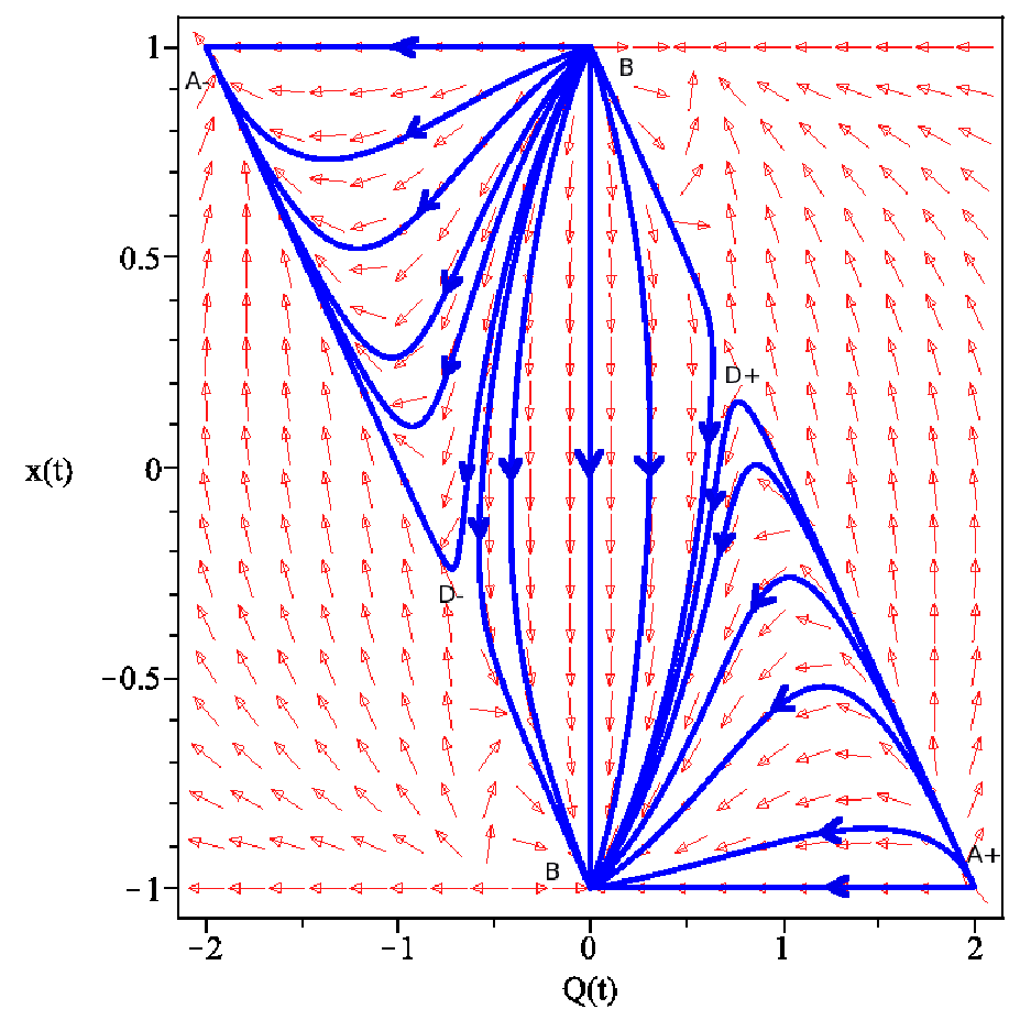
The non-invariant surface is the transition surface between accelerated and decelerated expansions phases (see Fig 1). By substituting 21 in 20 we obtain:
| (22) |
where . The evolution of the scale factor can now be given directly by integrating equation 22:
| (23) |
where
| (24) |
The constants of integration can be obtained by substituting the solutions into the original equations. As explained in [26], these solutions must satisfy all the cosmological equations in order to be considered physical.
By looking at Table 1 we can distinguish two classes of non - static solutions. The first class and } contain solutions that are independent of n and . The fixed point B represents a static phase as mentioned earlier, the points A, D and F are radiation - like phases. The expanding version of the point A is a saddle for and repeller for and the other two points D an F are saddles. The fixed point N represent a matter phase and the expanding version of this point is a spiral-.
The evolution of the scale factor a(t) for the fixed point is a function of and for fixed point is function of . The dependence of these solutions on n and/or provide us with additional degrees of freedom that can lead to interesting cosmological scenarios.
When , the fixed point merges with for , and it merges with the point for . When it merges with for , and for it corresponds to the matter point . In the case or , we find that for all values n for which this point is physical, the expansion (contraction) is never accelerating.
As mentioned earlier, the evolution of the scale factor for the point is independent of the equation of state parameter . For the fixed point merges with , for it merges with point and for it is a matter point.
We also find that for this fixed point the expansion (contraction) is accelerating for . The existence of this accelerated phase together with the fact that for the point is a matter-like point, leads to the possibility of an extremely interesting cosmological scenario, where it is possible in principle to find an orbit that starts close to the unstable accelerating phase , evolves past the unstable radiation - like point , followed by the unstable matter point and finally ends up at the de - Sitter attractor .
In Figs. 3 and 4 we have plotted two interesting orbits. The orbit in Fig 3 is for and . It begins near the radiation - like points , passes nearby the radiation - like point , followed by the standard matter point and ends up at the de-Sitter attractor . The orbit in Fig 4 is for and . It begins near the radiation - like point , passes nearby the matter point , then close to the matter point and ends up at the de Sitter attractor .
It is interesting to see that for all fixed points whose x - coordinate goes to zero as , are unstable. As the CDM subspace lies on the surface and this surface is not an invariant sub - manifold, this implies that the behavior of the solutions of a fourth order theory which is close to CDM, may be completely different from those of CDM. Furthermore, this suggests that the best fit model to the current observational data within the complete state space of , may be given by a non-infinitesimal value of .


VI Conclusion
In this work, we have presented a careful analysis of the state space of the class of theorys of gravity, focusing on the sector with , together with the no-ghost condition .
Due to the complexity of this class of gravity theories, the standard Hubble normalization does not lead to a compact dynamical variables. In order to construct variables defining a compact dynamical system one has to use an appropriate normalization. In this paper we used the same formalism used in [28], where we absorbed all the negative contributions of the Friedmann equation into the normalization. First of all we obtained the following important result: For all well defined function , with and invertible in terms of the dynamical variables defined by , the FLRW universes with non-negative Ricci Scalar, continues to be so both in the future and in the past. Also an R = 0 universe can never undergo a bounce in the future or past.
Our compact analysis shows that there are more equilibrium points than in the corresponding non-compact analysis in [26]. In particular we find a new finite fixed point . Because of it’s very special location in the phase space, it is quite difficult to obtain this point using the standard techniques. This point is found to represent a matter phase and the expanding version of this point is .
Furthermore, we find that for the phase space of , contains two accelerated fixed points , together with two other saddle points (one represent a radiation phase and the other represent a matter-like phase ). Although we have obtained all the desired fixed points and desired stability, this does not necessarily imply that there is an orbit connecting them. Due to the fact that for , the two accelerated points and the matter-like point are quite close to each other in the phase space, which makes it difficult to prove the existence of an orbit connecting these points together with the radiation - like point. But the presence of all these phases in the state space of makes a more detailed investigation worth pursuing.
References
- [1] J. P. Ostriker and P. J. Steinhardt, Cosmic Concordance, [arXiv:astro-ph/9505066].
- [2] S. Perlmutter et al., Astrophys. J. 517, 565 (1999); A. G. Riess et al., Astron. J. 116, 1009 (1998); J. L. Tonry et al., Astrophys. J. 594, 1 (2003); R. A. Knop et al., Astrophys. J. 598, 102 (2003); A. G. Riess et al. Astrophys. J. 607, 665 (2004); S. Perlmutter et al. Astrophys. J. 517, 565 (1999); Astron. Astrophys. 447, 31 (2006).
- [3] D. N. Spergel et al. Astrophys. J. Suppl. 148, 175 (2003); D. N. Spergel et al., Astrophys .J. Suppl. 170, 377 (2007).
- [4] M. Tegmark et al., Phys. Rev. D 69, 103501 (2004); U. Seljak et al., Phys. Rev. D 71, 103515 (2005); S. Cole et al., Mon. Not. Roy. Astron. Soc. 362, 505 (2005).
- [5] D. J. Eisenstein et al., Astrophys. J. 633, 560 (2005); C. Blake, D. Parkinson, B. Bassett, K. Glazebrook, M. Kunz and R. C. Nichol, Mon. Not. Roy. Astron. Soc. 365, 255 (2006).
- [6] B. Jain, A. Taylor, Phys. Rev. Lett. 91, 141302 (2003).
- [7] M. Dunajski and G. Gibbons, Class. Quant. Grav. 25, 235012 (2008) [arXiv:0807.0207 [gr-qc]].
- [8] A. A. Starobinsky, Phys. Lett. B 91, 99 (1980); K. S. Stelle, Gen. Rel. Grav. 9 353 (1978).
- [9] S. M. Carroll, V. Duvvuri, M. Trodden and M. S. Turner Phys. Rev. D70 043528 (2004); S. Nojiri and S. D. Odintsov Phys. Rev. D68, 123512 (2003); S. Capozziello, Int. Journ. Mod. Phys. D 11, 483 (2002); V. Faraoni Phys. Rev. D72, 124005 (2005); M. L. Ruggiero and L. Iorio JCAP 0701 010 (2007); A. de la Cruz-Dombriz and A. Dobado A, Phys. Rev. D74, 087501 (2006); N. J. Poplawski, Phys. Rev. D74, 084032 (2006); N. J. Poplawski, Class. Quantum Grav. 24, 3013 (2007); A. W. Brookfield, C. van de Bruck and L. M. H. Hall, Phys. Rev. D74, 064028 (2006); Y. Song, W. Hu and I. Sawicki Phys. Rev. D75, 044004 (2007); B. Li, K. Chan and M. Chu, Phys. Rev. D76, 024002 (2007); X. Jin, D. Liu and X. Li. [arXiv: astro-ph/0610854]; T. P. Sotiriou and S. Liberati S Ann. Phys. (NY) 322, 935 (2007); T. P. Sotiriou, Class. Quantum Grav. 23, 5117 (2006); R. Bean, D. Bernat, L. Pogosian, A. Silvestri and M. Trodden Phys. Rev. D75, 064020 (2007); I. Navarro and K. Van Acoleyen, JCAP 0702, 022 (2007); A. J. Bustelo and D. E. Barraco Class. Quantum Grav. 24, 2333 (2007); G. J. Olmo Phys. Rev. D75, 023511 (2007); J. Ford, S. Giusto and A. Saxena, Nucl. Phys. B 790, 258 (2008); F. Briscese, E. Elizalde, S. Nojiri and S. D. Odintsov, Phys. Lett. B646, 105 (2007); S. Baghram, M. Farhang and S. Rahvar, Phys. Rev. D75, 044024 (2007); D. Bazeia, B. Carneiro da Cunha, R. Menezes and A. Petrov Phys. Lett. B649, 445 (2007); P. Zhang Phys. Rev. D76, 024007 (2007); B. Li and J. D. Barrow Phys. Rev. Dbf 75, 084010 (2007); T. Rador, Phys. Lett. B 652, 228 (2007); T. Rador, Phys. Rev. D75, 064033 (2007); L. M. Sokolowski, Class. Quant. Grav. 24, 3391 (2007); V. Faraoni, Phys. Rev. D75, 067302 (2007); O. Bertolami, C. G. Boehmer, T. Harko and F. S. N. Lobo F S, Phys. Rev. D75, 104016 (2007); S. K. Srivastava, Int. J. Theor. Phys. 47, 1966 (2008); S. Capozziello, V. F. Cardone and A. Troisi, JCAP 08, 001 (2006); A. A. Starobinsky, JETP Lett. 86, 157 (2007); A. de Felice, S. Tsujikawa, f(R) theories, arXiv:1002.4928v1; E. Elizalde, S. D. Odintsov, L. Sebastiani, S. Zerbini, arXiv:1108.6184v1 [gr-qc]; E. Elizalde, S. Nojiri, S.D. Odintsov, L. Sebastiani, S. Zerbini, Phys.Rev. D 83 086006 (2011);S. Nojiri, S.D. Odintsov Phys.Rept. 505 59-144, (2011); S. Nojiri, S.D. Odintsov Int.J.Geom.Meth.Mod.Phys. 4 115-146, (2007).
- [10] R. Kerner Gen. Rel. Grav. 14, 453 (1982); J. P. Duruisseau, R. Kerner, Class. Quantum Grav. 3, 817 (1986).
- [11] P. Teyssandier, Class. Quantum Grav. 6 219 (1989).
- [12] G. Magnano, M. Ferraris and M. Francaviglia, Gen. Rel. Grav. 19 465 (1987).
- [13] S. Capozziello, V. F. Cardone, S. Carloni, A. Troisi, Int. J. Mod. Phys. D 12, 1969 (2003).
- [14] S. Capozziello, S. Carloni and A. Troisi, Recent Res. Devel. Astronomy & Astrophysics 1, 625 (2003).
- [15] S. Capozziello, V. F. Cardone, A. Troisi, JCAP 0608, 001 (2006).
- [16] Amare Abebe, Mohamed Abdelwahab, Alvaro de la Cruz-Dombriz, Peter K.S. Dunsby, [arXiv:1110.1191].
- [17] K. i. Maeda and N. Ohta, Phys. Lett. B 597, 400 (2004); K. i. Maeda and N. Ohta, Phys. Rev. D 71, 063520 (2005); N. Ohta, Int. J. Mod. Phys. A 20, 1 (2005); K. Akune, K. i. Maeda and N. Ohta, Phys. Rev. D 73, 103506 (2006).
- [18] S. Carloni, P. K. S. Dunsby, A. Troisi, Phys. Rev. D 77 024024 (2008); K. N. Ananda, S. Carloni, P. K. S. Dunsby, Phys. Rev. D 77, 024033 (2008); K. N. Ananda, S. Carloni, P. K. S. Dunsby, Class. Quant. Grav. 26 235018 (2009); K. N. Ananda, S. Carloni, P. K. S. Dunsby, A characteristic signature of fourth order gravity, [arXiv:0812.2028].
- [19] S. Capozziello, V.F. Cardone, A. Troisi, Mon. Not. Roy. Astron. Soc. 375, 1423 (2007).
- [20] J. Wainwright and G. F. R. Ellis (ed.), Dynamical Systems in Cosmology. Cambridge: Cambridge University Press. ISBN 0-521-55457-8.
- [21] http://www.mth.uct.ac.za/peter/coordinates.pdf
- [22] S. Carloni, P. K. S. Dunsby, S. Capozziello, A. Troisi, Class. Quant. Grav. 22, 4839 (2005); S. Carloni and P. K. S. Dunsby, J. Phys. A 40, 6919 (2007); S. Carloni, A. Troisi, P. K. S. Dunsby, Gen. Rel. Grav. 41, 1757 (2009).
- [23] B. de Witt, Dynamical Theory of Groups and Fields (New York: Gordon and Breach, 1965)
- [24] Birrell N, Davies P 1982 Quantum Fields in Curved Space (Cambridge: Cambridge Univ. Press)
- [25] Pechlaner E and Sex1 R 1966 Commun. Math. Phys. 2 165
- [26] S. Carloni, K. N. Ananda, P. K. S. Dunsby and M. E. S. Abdelwahab, arXiv:0812.2211 [astro-ph].
- [27] N. Goheer, J. A. Leach and P. K. S. Dunsby, Class. Quant. Grav. 25, 035013 (2008).
- [28] N. Goheer, R. Goswami, and P. K. S. Dunsby, Class. Quant. Grav. 26, 105003 (2009).