Two-dimensional self-avoiding walks and polymer adsorption: Critical fugacity estimates

Self-avoiding walks (SAW) in a half-space, originating at a site on the surface, are well-known and useful models of polymer adsorption, see [11, 21] for reviews. It is known [20] that the connective constant for such walks is the same as for the bulk case. To model surface adsorption, one adds a fugacity $y={\rm e}^{\alpha}$ to sites or edges in the surface. Let $c_{n}^{+}(m)$ be the number of half-space walks of $n$-steps, with $m$ monomers in the surface, and define the partition function as

with $\alpha=-\epsilon/k_{B}T,$ where $\epsilon$ is the energy associated with a surface site (or edge), $T$ is the absolute temperature and $k_{B}$ is Boltzmann’s constant. If $\epsilon$ is sufficiently large and negative, the polymer adsorbs onto the surface, while if $\epsilon$ is positive, the walk is repelled by the surface. It has been shown by Hammersley, Torrie and Whittington [10] in the case of the $d$-dimensional hypercubic lattice that the limit

exists, where $\kappa(\alpha)$ is the reduced, intensive, free-energy of the system. It is a convex, non-decreasing function of $\alpha,$ and therefore continuous and almost everywhere differentiable. Their discussion and proof apply, mutatis mutandis to the honeycomb and triangular lattices.

In the case of the honeycomb lattice there are two types of surface sites, marked as solid and empty circles in Figure 1. In most studies just one of the the two types is weighted; namely, those marked with solid circles in Figure 1. In this study we also allow for a surface weight on the second type of sites and we study the case where all surface sites carry the same weight.

For $\alpha<0,$ $\kappa(\alpha)=\log\mu$ [20], where $\mu$ is the connective constant for SAW on the given lattice. For $\alpha\geq 0,$

This behaviour implies the existence of a critical value $\alpha_{\rm c},$ such that, for the hyper-cubic lattice, $0\leq\alpha_{\rm c}\leq\log\mu.$ The situation as $\alpha\to\infty$ has only recently been rigorously established by Rychlewski and Whittington [19], who proved that $\kappa(\alpha)$ is asymptotic to $\alpha$ in this regime. As illustrated in Figure 1, it is convenient to attach weights $y$ to only half of the sites along the surface to allow for simplifications later on. In this case the bounds on $\alpha_{\rm c}$ become $0\leq\alpha_{\rm c}\leq 2\log\mu$, or equivalently $1\leq y_{\rm c}={\rm e}^{\alpha_{\rm c}}\leq\mu^{2}$.

Various other quantities exhibit singular behaviour at $y_{\rm c}$. For example, the mean density of sites in the surface is given by

In the limit of infinitely long walks one has

From the behaviour of $\kappa$ given above, it can be seen that $\rho(\alpha)=0$ for $y<y_{\rm c}$ and $\rho(\alpha)>0$ for $y>y_{\rm c}.$

In a recent paper Beaton, de Gier and Guttmann [2] generalised a finite lattice identity by Duminil-Copin and Smirnov [6] for the honeycomb lattice to the case where weights are introduced on alternating sites along a boundary as represented by the solid circles in Figure 1. This resulted in a proof of a conjecture of Batchelor and Yung [1] that the critical surface fugacity of self-avoiding walks interacting with (alternate) sites on the surface of the honeycomb lattice is $1+\sqrt{2}.$ Here we briefly outline the results.

Let $H$ be the set of mid-edges on a half-plane of the honeycomb lattice. We define a domain $\Omega\subset H$ to be a simply connected collection of mid-edges. The set of sites adjacent to the mid-edges of $\Omega$ is denoted $V(\Omega)$. Those mid-edges of $\Omega$ which are adjacent to only one site in $V(\Omega)$ form $\partial\Omega$. Since surface interactions are the focus of this article, we will insist that at least one site of $V(\Omega)$ lies on the boundary of the half-plane.

Let $\gamma$ be a self-avoiding walk in a domain $\Omega.$ We denote by $\ell(\gamma)$ the number of sites occupied by $\gamma$, and by $\nu(\gamma)$ the number of contacts with the boundary. Define the following observable: for $a\in\partial\Omega,z\in\Omega$, set

where the sum is over all configurations $\gamma\subset\Omega$ for which the SAW goes from the mid-edge $a$ to a mid-edge $z$. $W(\gamma(a\rightarrow z))$ is the winding angle of that self-avoiding walk. See Figure 1 for an example – the SAW shown there starts on the central mid-edge of the left boundary (shown as $a$) and ends at a mid-edge $z$. As the SAW runs from mid-edge to mid-edge, it acquires a weight $x$ for each step and a weight $y$ for each contact (shown as a solid circle) with the right hand side boundary.

We define the following generating functions:

where the sums are over all configurations that have a contour from $a$ to the $\alpha$, $\beta$ or $\varepsilon,\bar{\varepsilon}$ boundaries respectively. For the SAW model in the dilute regime, the result proved in [2] for the $n$-vector model simplifies (in the case $n=0$) to:

where

A simple corollary of (1) is that at $y=y^{*}$ we have

The importance of this result is that the generating function $B_{T,L}$ for $y=y^{*}$ has disappeared from (2). In [2] we proved that the critical surface fugacity $y_{c}$ is equal to $y^{*}$. Using this result and taking the limit $L\to\infty,$ the geometry becomes a strip of width $T,$ and the corollary then becomes

In [2], we also proved that $E_{T}(x_{c},y)=0$ for all $0\leq y\leq y_{c}.$ So (3) simplifies further to

This is a remarkable equation in that it implies that $y_{\rm c}$ can be identified from the generating function $A_{T}(x_{c},y)$ for any width $T,$ simply by solving equation (4). To show the power of this observation, note that virtually by inspection one can write down the solution for strip width $0,$ which is

Solving $1/\cos\left(\frac{3\pi}{8}\right)=A_{0}(x_{\rm c},y),$ recalling $x_{c}=1/\sqrt{2+\sqrt{2}},$ gives $y=y_{\rm c}=1+\sqrt{2},$ the exact value of the critical fugacity.

For other lattices, and even for the honeycomb lattice with interactions at every surface site, we do not have an equivalent identity, such as $1=c_{\alpha}A_{T}(x_{\rm c},y_{\rm c}).$ However if one plots $A_{T}(x_{\rm c},y)$ versus $y$ in these cases, one might be forgiven for thinking that such an identity exists. In Figure 3 we show a plot of $A_{T}(x_{\rm c},y)$ versus $y,$ for a range of strip widths $T.$ To graphical accuracy it appears that there is a unique point of intersection for plots corresponding to higher values of $T$. Even finer resolution, see inset, suggests that this is the case. The actual small deviation can be seen from the data given in Table 4.

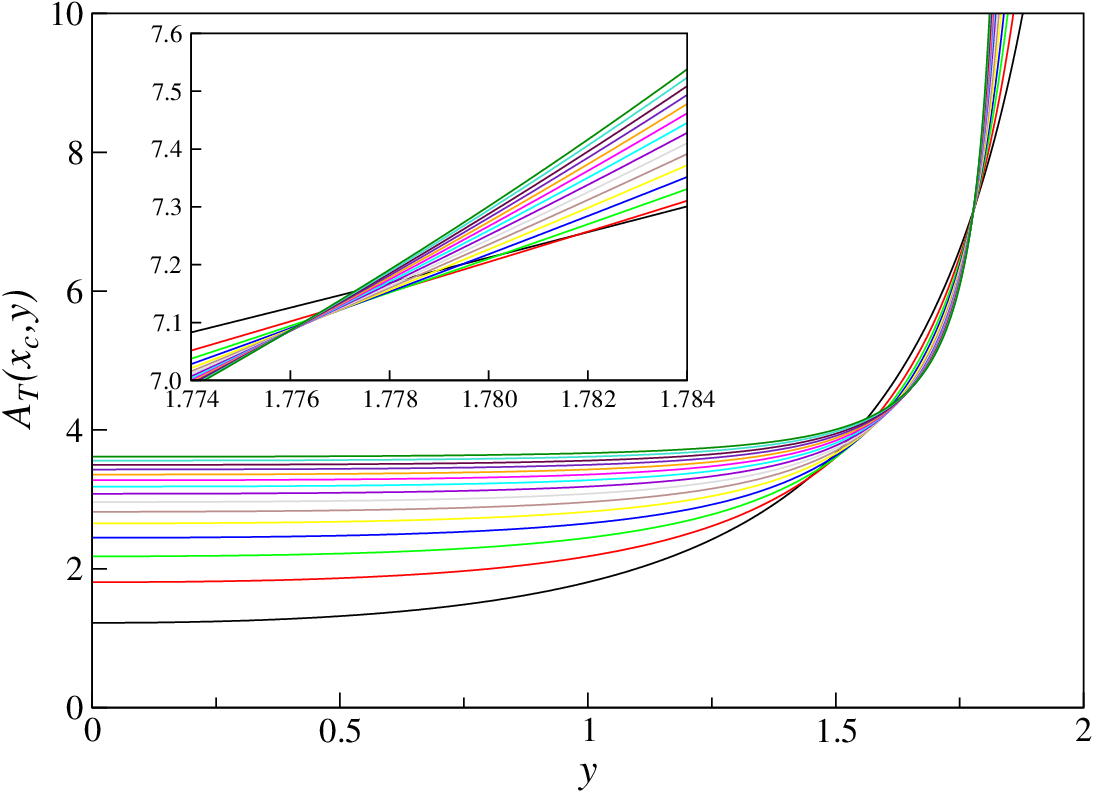
We denote by $y_{c}(T)$ the point of intersection of $A_{T}(x_{\rm c},y)$ and $A_{T+1}(x_{\rm c},y).$ We observe that the sequence $\{y_{c}(T)\}$ is a monotone function of $T.$ We argue, as in [3], that in the scaling limit all two dimensional SAW models are given by the same conformal field theory. Since it is known for one of these models (i.e. honeycomb lattice SAW with alternate site interactions) that the critical point can be found by requiring certain contour integrals to vanish, it follows that in the scaling limit the same should be true for all two dimensional SAW¹¹ 1 We thank John Cardy for this observation.. This is entirely consistent with our observations, and implies that $\lim_{T\to\infty}y_{c}(T)=y_{c}.$

This then suggests a potentially powerful new numerical approach to estimating $y_{c}.$ One calculates the generating functions $A_{T}(x_{\rm c},y),$ for all strip widths $T=0,1,2,\ldots T_{\rm max},$ uses these to calculate $y_{c}(T)$ for $T=0,1,2,\ldots T_{\rm max-1}$ as defined above, and then extrapolates this monotone sequence by a variety of standard sequence extrapolation methods. A similar idea was used to furnish estimates of $x_{c}$ in [3].

In Section 3 we describe the derivation of the generating functions $A_{T}(x_{c},y)$ by the finite-lattice method for a range of strip widths $T$ that are needed in this study. For the value of the critical step fugacity $x_{c},$ we use the exact result $x_{c}=1/\sqrt{2+\sqrt{2}}$ for the honeycomb lattice, and the best available series estimates in the case of the square and triangular lattices. These are $x_{c}({\rm sq})=0.37905227776$ [17, 13], with uncertainty in the last digit, and $x_{c}({\rm tr})=0.2409175745$ [15], with similar uncertainty. We performed a sensitivity analysis of our critical surface fugacity estimates in order to determine how sensitive they are to uncertainties in our estimates of $x_{c}.$ The estimates of $x_{c}$ are sufficiently precise that a change in our estimate of $x_{c}$ by a factor of 10 times the estimated uncertainty will not change our estimates of the surface fugacity $y_{c}$ in even the least significant digit.

In Section 4 we estimate the critical fugacity by extrapolating $y_{c}(T)$ using a range of standard extrapolation algorithms. These are Levin’s $u$-transform, Brezinskii’s $\theta$ algorithm, Neville tables, Wynn’s $\epsilon$ algorithm and the Barber-Hamer algorithm. Descriptions of these algorithms, and codes for their implementation, can be found in [9]. However, we find the most precise estimates are given by the Bulirsch-Stoer algorithm [4]. This algorithm requires a parameter $w$, which can be thought of as a correction-to-scaling exponent. For the purpose of the current exercise, we have set this parameter to $1$, corresponding to an analytic correction, which is appropriate for the two-dimensional SAW problem [5]. Our implementation of the algorithm is precisely as described by Monroe [18], and we retained 50 digit precision throughout.

We used this method to estimate the critical fugacity for all cases of interest for two-dimensional SAWs. For the honeycomb lattice, discussed in Subsection 4.1, we have already proved [2] that $y_{c}=1+\sqrt{2}$ for the alternate site interaction model, as conjectured by Batchelor and Yung [1]. It is a straightforward consequence of this result – the argument is given in Subsection 4.1 below – that for the honeycomb lattice with surface edge interactions (rather than site interactions), the critical fugacity is $\sqrt{1+\sqrt{2}}.$ For the honeycomb lattice site interaction problem where every surface site interacts with the walk, we find the critical fugacity to be $y_{c}=1.46767$ where the error in this estimate (and all such estimates given below), is expected to be confined to a few parts in the last quoted digit. We know of no other estimate of this quantity in the literature.

In subsection 4.2 we discuss the critical fugacity for site and edge weighted adsorption on the square lattice. The only previous estimates for the site weighted case can be found in [12], where Monte Carlo methods were used to obtain the estimate $y_{c}=1.76\pm 0.02.$ Our estimate, $y_{c}=1.77564$ is three orders of magnitude more precise than this. For the edge weighted case, a transfer matrix estimate is given in [8], and is $y_{c}=2.041\pm 0.002.$ In [7] a Monte Carlo estimate of comparable precision is given, $y_{c}=2.038\pm 0.002.$ Our estimate is $y_{c}=2.040135,$ again some three orders of magnitude more precise.

For the triangular lattice, discussed in Subsection 4.3 we are unaware of any previous investigations of the critical fugacity. We find, in Section 4.3, that $y_{c}({\rm site})=2.144181$ and $y_{c}({\rm edge})=2.950026.$ We repeat that errors in our quoted estimates are expected to be confined to a few parts in the last quoted digit.

The algorithms we use to enumerate SAW interacting with a surface on the honeycomb, square and triangular lattices builds on the algorithm outlined in our previous paper [3] and detailed descriptions can be found in these papers [14, 15, 16]. Suffice to say that the generating functions for a given strip were calculated using transfer matrix (TM) techniques. The most efficient implementation of the TM algorithm generally involves bisecting the finite lattice with a boundary (this is just a line in our case) and moving the boundary in such a way as to build up the lattice site by site. If we draw a SAW and then cut it by a line we observe that the partial SAW to the left of this line consists of a number of loops connecting two edges in the intersection, and at most two unconnected or free edges. The other end of the free edge is an end-point of the SAW, hence there are at most two free ends.

The sum over all contributing graphs is calculated as the boundary is moved through the lattice. For each configuration of occupied or empty edges along the intersection we maintain a generating function $G_{S}$ for partial walks with configuration $S$. In exact enumeration studies $G_{S}$ would be a truncated two-variable polynomial $G_{S}(x,y)$ where $x$ is conjugate to the number of steps and $y$ to the number of surface-contacts (sites or edges). In a TM update each source configuration $S$ (before the boundary is moved) gives rise to a few new target configurations $S^{\prime}$ (after the move of the boundary line) and $n=0,1$ or 2 new edges and $m=0$ or 1 new contacts are inserted leading to the update $G_{S^{\prime}}(x,y)=G_{S^{\prime}}(x,y)+x^{n}y^{m}G_{S}(x,y)$. Here we are primarily interested in the case where $A(x,y)$ or $B(x,y)$ are evaluated at the critical point $x=x_{c}$. This actually makes life easier for us since we can change to a single variable generating function $G_{S}(y)$ and update signatures as $G_{S^{\prime}}(y)=G_{S^{\prime}}(y)+x_{c}^{n}y^{m}G_{S}(y)$. Here $G_{S}(y)$ is a polynomial in the contact fugacity $y$ with real coefficients truncated at some maximal degree $M$. The calculations were carried out using quadruple (or 128-bit) floating-point precision (achieved in FORTRAN with the REAL(KIND=16) type declaration).

In our calculations we truncated $A(x_{c},y)$ at degree $M=1000$ and used strips of half-length $L=M$. In Table 1 we have listed estimates for $y_{c}(9)$ obtained from strips of width 10 and 9 (the crossing between $A_{10}(x_{c},y)$ and $A_{9}(x_{c},y)$) for various values of $M$ and $L$. Clearly the choice $M=L=1000$ suffices to estimate $y_{c}(9)$ to more than 10 digits accuracy.

The transfer-matrix algorithm is eminently suited for parallel computations and here we used the approach first described in [13] and refer the interested reader to this publication for further detail. The bulk of the calculations for this paper were performed on the cluster of the NCI National Facility, which provides a peak computing facility to researchers in Australia. The NCI peak facility is a Sun Constellation Cluster with 1492 nodes in Sun X6275 blades, each containing two quad-core 2.93GHz Intel Nehalem CPUs with most nodes having 3GB of memory per core (24GB per node). It took a total of about 3300 CPU hours to calculate $A_{T}(x_{c},y)$ for $T$ up to 15 on the square lattice. It is known [14] that the time and memory required to obtain the number of walks in a strip of width $T$ grows exponentially as $3^{T}$ for the honeycomb and square lattices and as $4^{T}$ for the triangular lattice. So, the bulk of the time was spent calculating $A_{15}$ and $B_{15}$, which amounted to almost 2300 hours in the square lattice case. In this case we used 48 processors and the split between actual calculations and communications was roughly 2 to 1 (with quite a bit a variation from processor to processor). Smaller widths can be done more efficiently in that communication needs are lesser and hence not as much time is used for this task.

We have estimated the critical fugacity for surface adsorption for two-dimensional SAW on all regular lattices for both the case of site and edge interactions. Many of these estimates are new. Those that are not are several orders of magnitude more precise than pre-existing estimates. Uniquely for the case of the honeycomb lattice with edge interactions, we give the exact value of the critical fugacity, and also prove it. Our results are summarised in Table 7.

AJG and IJ acknowledge financial support from the Australian Research Council. NRB was supported by the ARC Centre of Excellence for Mathematics and Statistics of Complex Systems (MASCOS). This work was supported by an award under the Merit Allocation Scheme on the NCI National Facility at the ANU.

References

- [1] M T Batchelor and C M Yung, Exact results for the adsorption of a flexible self-avoiding polymer chain in two dimensions, Phys. Rev. Letts 74, 2026-9 (1995).
- [2] N R Beaton, J de Gier and A J Guttmann, The critical fugacity for surface adsorption of SAW on the honeycomb lattice is arXiv:1109:1234 (2011).
- [3] N R Beaton, A J Guttmann and I Jensen, A numerical adaptation of SAW identities from the honeycomb to other 2D lattices, arXiv:1110.1141v2 (2011).
- [4] R Bulirsch and J Stoer, Fehlerabschätzungen und Extrapolation mit rationalen Funktionen bei Verfahren vom Richardson-Typus, Numer. Math. 6, 413–27 (1964).
- [5] S Caracciolo, A J Guttmann, I Jensen, A Pelissetto, A N Rogers and A D Sokal, Correction-to-scaling exponents for two-dimensional self-avoiding walks, J Stat Phys 120, Nos 5/6, 1037–1100 (2005).
- [6] H Duminil-Copin and S Smirnov, The connective constant of the honeycomb lattice equals arXiv:1007.0575 (2010).
- [7] P Grassberger and R Hegger, Comment on “Surface critical exponents of self-avoiding walks on a square lattice with an adsorbing linear boundary: A computer simulation study”, Phys. Rev. E, 51, 2674-6 (1995)
- [8] I Guim and T W Burkhardt, Transfer matrix study of the adsorption of a flexible self-avoiding polymer chain in two dimensions, J. Phys. A: Math. Gen 22, 1131–40 (1989).
- [9] A J Guttmann, Analysis of coefficients, in Phase transitions and critical phenomena Vol. 13 p. 1, eds C Domb and J L Lebowitz, Academic Press, London and NY (1989).
- [10] J M Hammersley, G M Torrie and S G Whittington, Self-avoiding walks interacting with a surface, J. Phys. A: Math. Gen 15, 539-71 (1982).
- [11] E J Janse van Rensburg, The statistical mechanics of interacting walks, polygons, animals and vesicles, OUP, Oxford (2000).
- [12] E J Janse van Rensburg and A R Rechnitzer, Multiple Markov chain Monte Carlo study of adsorbing self-avoiding walks in two and three dimensions. J. Phys. A: Math. Gen 37, 6785–98 (2004).
- [13] I Jensen, A parallel algorithm for the enumeration of self-avoiding polygons on the square lattice, J. Phys. A: Math. Gen. 36, 5731–45 (2003).
- [14] I Jensen, Enumeration of self-avoiding walks on the square lattice, J. Phys. A: Math. Gen. 37, 5503–24 (2004).
- [15] I Jensen, Self-avoiding walks and polygons on the triangular lattice, J. Stat. Mech.:Th. and Exp., P10008 (2004).
- [16] I Jensen, Honeycomb lattice polygons and walks as a test of series analysis techniques, J. Phys.: Conf. Ser. 42, 163-72 (2006).
- [17] I Jensen and A J Guttmann, Self-avoiding polygons on the square lattice, J. Phys. A: Math. Gen. 31, 4867-76 (1999).
- [18] J L Monroe, Extrapolation and the Bulirsch-Stoer algorithm Phys. Rev. E 65, 066116 (8pp) (2002).
- [19] G Rychlewski and S G Whittington, Self-avoiding walks and polymer adsorption: low temperature behaviour, J. Stat. Phys. 144 in press (2011).
- [20] S G Whittington, Self-avoiding walks terminally attached to an interface, J. Chem. Phys. 63, 779-85 (1975).
- [21] C Vanderzande, Lattice Models of Polymers, Cambridge Lecture Notes in Physics 11, (Cambridge University Press, 1998).