The Rest Frame UV to Optical Colors and SEDs of $z\sim 4-7$ galaxies.

Valentino González, Rychard J. Bouwens, Ivo Labbé, Garth Illingworth, Pascal Oesch, Marijn Franx, Dan Magee Alternate Affiliation: Astronomy Department, University of California, Santa Cruz, CA 95064 Alternate Affiliation: Leiden Observatory, Leiden University , NL-2300 RA Leiden, Netherlands Alternate Affiliation: Hubble Fellow

Abstract

We use the ultra-deep HUDF09 and the deep ERS data from the HST WFC3/IR camera, along with the wide area $Spitzer$ /IRAC data from GOODS-S to derive SEDs of star-forming galaxies from the rest-frame UV to the optical over a wide luminosity range ( $M_{1500}\sim-21$ to $M_{1500}\sim-18$ ) from $z\sim 7$ to $z\sim 4$ . The sample contains $\sim 400\ z\sim 4$ , $\sim 120\ z\sim 5$ , $\sim 60\ z\sim 6$ , and 36 prior $z\sim 7$ galaxies. Median stacking enables the first comprehensive study of very faint high-z galaxies at multiple redshifts (e.g., $[3.6]=27.4\pm 0.1$ AB mag for the $M_{1500}\sim-18$ sources at $z\sim 4$ ). At $z\sim 4$ our faint median-stacked SEDs reach to $\sim 0.06L^{*}_{z=4}$ and are combined with recently published results at high luminosity $L>L^{*}$ that extend to $M_{1500}\sim-23$ . We use the observed SEDs and template fits to derive rest frame UV-to-optical colors $(U-V)$ at all redshifts and luminosities. We find that this color does not vary significantly with redshift at a fixed luminosity. The UV-to-optical color does show a weak trend with luminosity, becoming redder at higher luminosities. This is most likely due to dust. At $z\gtrsim 5$ we find blue colors $[3.6]-[4.5]\sim-0.3\,$ mag that are most likely due to rest-frame optical emission lines contributing to the flux in the IRAC filter bandpasses. The scatter across our derived SEDs remains substantial, but the results are most consistent with a lack of any evolution in the SEDs with redshift at a given luminosity. The similarity of the SEDs suggests a self-similar mode of evolution over a timespan from 0.7 Gyr to 1.5 Gyr that encompasses very substantial growth in the stellar mass density in the universe (from $\sim 4\times 10^{6}$ to $\sim 2\times 10^{7}$ ${\rm M_{\odot}Mpc^{-3}}$ )

Subject headings

galaxies: evolution — galaxies: high-redshift

I. Introduction

As a result of the installation of the WFC3/IR camera on the Hubble Space Telescope, it is now possible to obtain extremely deep, high resolution observations in the near infrared. These observations match the exquisite optical data provided by the ACS camera over deep and ultra-deep fields like the GOODS and the HUDF [21, 5]. The upgrade has enabled several teams to extend their searches for Lyman Break Galaxies (LBGs) to very high redshifts [8, 35, 36, 31, 51, 12, 18, e.g.,]. In combination, these two cameras have allowed for high S/N measurements of the rest-frame UV light of high redshift galaxies over a wide wavelength baseline.

As a result of these new observations, the UV LFs at $z\gtrsim 4$ are known to high accuracy. Another direct result from these observations is the determination of the UV slope of the SEDs, generally characterized by the parameter $\beta$ ( $f_{\lambda}\propto\lambda^{\beta}$ , e.g., Meurer et al. 33, Bouwens et al. 4). This slope has been shown to become steeper (bluer colors) both with decreasing luminosity and with increasing redshift (Bouwens et al. 4, Bouwens et al. 6, Wilkins et al. 48, but see Dunlop et al. 14, Finkelstein et al. 19). For a mid-aged ( $100\,$ Myr) stellar population, this slope generally depends most strongly on the dust reddening so this has been interpreted as an increase in the dust content of galaxies with cosmic time and as galaxies increase in luminosity [6, 19].

Since the rest-frame UV light primarily probes young short-lived stellar populations (mostly O and B stars), it is interesting to extend these observations to longer wavelengths and study the relative importance of more evolved stellar populations. This is very challenging though and is now only possible thanks to the incredible sensitivity of the IRAC camera on the $Spitzer$ Space Telescope. Some of the first observations of rest-frame optical light from $z\gtrsim 4$ galaxies showed quite substantial UV-to-optical colors [17, 50]. Under the usual assumption of smooth, exponentially declining star formation histories (SFHs), these colors were interpreted as indicative of an evolved stellar population (ages $\gtrsim 100\,$ Myr) in combination with the younger populations probed by the UV-light. Follow-up work on $z\sim 4-7$ galaxies continued to reveal systems with moderate size UV-to-optical breaks [16, 49, 26, 45, 23, e.g.], even possibly to $z\sim 8$ [27]. However interesting, these studies are only possible for the brightest $z>4$ galaxies, due to the extreme depths required.

Some alternative explanations have been proposed for the red UV-to-optical colors observed in $z>6$ galaxies. For example, for young star-froming galaxies, one might expect strong line emission. At the right redshift, these lines could contaminate the 3.6 and 4.5 $\mu m$ IRAC fluxes, resulting in red UV-to-optical colors similar to those produced by the Balmer break [42, 43]. For emission lines to be strong enough to dominate the rest-frame optical fluxes, extremely young ages ( $\sim 6\,$ Myr) are required. Such models have ages shorter than the dynamical times of these high $-z$ sources and are also somewhat uncertain. It would be surprising if the majority of these galaxies, which are selected over a redshift range that spans $\gtrsim 200\,$ Myr, had such young ages. Even if rest-frame optical emission nebular emission lines do not dominate the measured IRAC fluxes, it is expected that they will contribute some of the flux measured in the mid-IR, but the exact contribution currently remains hard to establish at these high redshifts.

It has been routine, then, to compare the colors of these high redshift galaxies with synthetic stellar population (SSP) models of relatively evolved galaxies with smooth SFHs to derive physical properties from the observations. By studying LBG samples at different redshifts in the aforementioned way, one intriguing result has emerged. At a given intrinsic luminosity, the specific Star Formation Rate (SFR) of galaxies seems to remain remarkably constant with redshift (Stark et al. 45, González et al. 23, González et al. 22, McLure et al. 32; slightly modified to account for the latest dust corrections by Bouwens et al. 6). This result has called the attention of theorists and has proved very hard to reproduce in simulations [47, 24, e.g.,]. The assumptions used to derive these result vary somewhat from group to group. In this work, we present the basic observations that lead to such a result, namely the observed SEDs of galaxies at $z\sim 4-7$ .

In the present work we study the observational properties of the typical high redshift galaxy. We do this by splitting our large sample in both redshift and UV-luminosity bins and constructing mean SEDs. The large number of galaxies allows us to study the typical colors at high S/N but also extend our measurements to faint limits that are currently inaccessible on an individual basis with the current data. Although the scatter about the typical properties is also highly interesting, we defer their study to a future work which relies on even deeper $Spitzer$ observations. In section 2 we present the Data and in section 3 the sample selection and photometry. Section 4 describes the stacking procedure and we discuss the stacked SEDs and colors in section 5. A summary is presented in section 6.

Throughout, we use a ( $H_{0},\,\Omega_{M},\,\Omega_{\Lambda}$ ) = ( $70\,\rm{km~s^{-1}}$ , 0.3, 0.7) cosmology when necessary and we quote all magnitudes in the AB system [37].

Table 1Sample Summary.

	$z\sim 4$	$z\sim 5$	$z\sim 6$	$z\sim 7\tablenotemark{a}$
ERS	270 / 524	77 / 123	20 / 32	15 / 18
HUDF	137 / 205	41 / 55	38 / 51	21
TOTAL	407 / 729	118 / 178	58 / 83	36

Note. — Summary of the number of sources in the sample. IRAC photometry of these sources requires fitting and subtraction of the flux from surrounding foreground neighbors. This is not possible in all the cases. The table shows the number of sources with clean IRAC photometry / total number of sources found in the field.

Refer to caption — Figure 1.— The observed magnitude distribution of the sample. The reference filters for each redshift sub-sample have been chosen to be close to rest-frame $\lambda=1500\,$ Å. For the $z\sim 6$ sources in the ERS we used the $Y_{98}$ filter whereas the $Y_{105}$ filter was used for the sources in the HUDF. The open histograms include all the sources and the gray filled histograms include only the sources with clean IRAC photometry. This selection does not introduce biases relevant to the determination of the mean rest-frame optical colors of these sources.

II. Data

In this paper, we make use of the large number of $z\gtrsim 4$ galaxies found in the ultra-deep HUDF data and wide-area ERS data to construct median SEDs for star-forming galaxies at $z\sim 4-7$ . The deep optical, near-IR, and deep IRAC coverage over these fields allow us to create SEDs that cover both the rest-frame UV and the rest-frame optical down to very faint fluxes.

II.1. HST ACS and WFC3/IR

In constructing our median SEDs, we make use of the deep optical and near-IR HST data from ACS and WFC3/IR. Over the ERS field, both the ACS optical ( $B_{435}$ $V_{606}$ $i_{775}$ $z_{850}$ ) and the WFC3/IR ( $Y_{98}$ $J_{125}$ $H_{160}$ ) images from HST reach depths of $\sim 28$ mag ( $5\,\sigma$ measured on 0.35″-diameter apertures). In the HUDF field, the ACS optical data ( $BViz$ ) are $1.5-2$ mags deeper, and the WFC/IR data ( $Y_{105}J_{125}H_{160}$ ) are 1.5 times deeper than the ERS. The HUDF was observed with the $Y_{105}$ filter instead of the $Y_{98}$ filter used in the ERS.

II.2. Spitzer/IRAC

Because these fields are located inside the GOODS-S field, they both have deep $Spitzer$ /IRAC coverage that amounts to $\sim 23.3\,$ hr over the ERS and twice that for the HUDF which was observed to the same depths but in two different epochs with the IRAC camera rotated by $180^{\circ}$ . For IRAC channel 1 images ( $\lambda_{\circ}=3.6\mu m$ ), each single epoch reaches depths of 27.8 mags, measured over 2.5″-diameter apertures ( $1\,\sigma$ ). For channel 2 ( $\lambda_{\circ}=4.5\mu m$ ) this limit corresponds to 27.2 mags.

III. Sample Selection and Basic Photometry

The criteria used to identify high redshift star forming galaxies has already been presented in numerous previous works. For details on the selection procedure and discussion of sample contamination please see Bouwens et al. [5], Bouwens et al. [7]. In short, the selection criteria used to find the sources presented here is as follows:

$z\sim 4~B$ -dropouts:

(B_{435}-V_{606}>1.1)~\wedge~[B_{435}-V_{606}>(V_{606}-z_{850})+1.1]

\wedge~(V_{606}-z_{850}<1.6)

$z\sim 5~V$ -dropouts:

\{[V_{606}-i_{775}>0.9(i_{775}-z_{850})]~\vee~(V_{606}-i_{775}>2)\}

\wedge~(V_{606}-i_{775}>1.2)~\wedge~(i_{775}-z_{850}<1.3)

$z\sim 6~i$ -dropouts:

(i_{775}-z_{850}>1.3)~\wedge~(z_{850}-J_{125}<0.8)

The combined samples contain a total of 729 sources at $z\sim 4$ , 178 at $z\sim 5$ , and 83 at $z\sim 6$ (see table 1).

We complement the $z\sim 4,~5$ , and 6 samples with the sample of 36 $z\sim 7$ sources presented by Labbé et al. [27]. We have adopted the $z\sim 7$ stacks presented in that work.

At these depths, the $Spitzer$ /IRAC images are fairly crowded due to the size and shape of its PSF. As a consequence, standard aperture photometry of the sources generally results in fluxes that are contaminated by flux coming from unrelated sources that are nearby in the sky. We are able to de-blend the fluxes from the different sources by making use of the higher resolution information available through the HST images. Our method has been explained in previous works by our group [26, 28, 23, 22, e.g] but we give a short description here. We start by registering the IRAC images to the higher resolution HST image that will be used as a light profile template. In this case we use the WFC3/IR $H_{160}$ -band image as our template because it is the closest in wavelength and has high signal to noise. We use the SExtractor software [3] to create segmentation maps. We isolate all the sources in a small area around each galaxy in our sample using these segmentation maps. We then convolve them with a kernel derived from the PSFs of the HST and the IRAC images. We fit for the normalization fluxes of all sources (including the source we are trying to clean) simultaneously. Finally we remove the flux from the unrelated sources to obtain a clean image of the galaxies in our sample. Later we use these cleaned images to produce median stacks.

The procedure described above does not always produce acceptable results. The reasons why it can fail vary but the most common is the presence of a source that is too bright, extended, and close to our region of interest. In these cases the amount of flux subtracted off our source of interest is large and more uncertain and in most cases results in large residuals. We have carefully inspected the residual images (all sources subtracted, including the one in our sample) and the cleaned images (only unrelated neighbors subtracted) of each of the sources in the original sample and come up with a sub-sample of sources with clean IRAC photometry. This “by eye” inspection criterion generally results in good agreement with a criterion that selects only the images with the lowest $\chi^{2}$ residuals but allows us to also remove sources that, even though have moderate $\chi^{2}$ values, present mild to strong residuals located very close to the source. Overall, this reduces the sample to 60% of the original (see Table 1). Since the criterion adopted here depends on the complexity of the unrelated sources, it is not expected that it should introduce any biases that would be relevant in the determination of the mean rest-frame optical colors (see Figure 1).

IV. Stacked Photometry and Median SEDs

It has been shown that in star forming galaxies the total SFR appears to correlate with stellar mass, the so called main sequence of star forming galaxies [34]. This sequence has been observed at high-redshifts ( $z\gtrsim 4$ ) but contrary to what has been observed at $z<2$ , the normalization of the relation at fixed stellar mass does not seem to evolve over $2<z<7$ [45, 22]. The lack of deeper rest-frame optical from $Spitzer$ /IRAC for these sources is one of the big limitations to study this sequence to fainter magnitudes. In terms of the bulk of the population, however, progress can be made by stacking large numbers of sources to study their mean properties. In this section we seek to construct the median SEDs of galaxies at $z\gtrsim 4$ .

Due to the nature of the dropout search and the filters available, our full sample is naturally divided in redshift bins centered at $\langle z\rangle=3.8,5.0,5.9$ plus the $\langle z\rangle=6.9$ sample from Labbé et al. [27]. In this section, we further split each redshift sub-sample based on their observed rest-frame UV-luminosity. The filters used as reference UV-luminosity are the $i_{775}$ filter for the $z\sim 4$ sources; the $z_{850}$ for the $z\sim 5$ sources; the $Y_{98}$ for the $z\sim 6$ sources in the ERS and the $Y_{105}$ for the $z\sim 6$ sources in the HUDF; and finally, the $J_{125}$ filter the $z\sim 7$ sources. These filters were chosen to be close to rest-frame 1500 Å at the different redshifts and make the splitting criterion fairly uniform across redshifts. These bins are presented in Figure 1.

In the case of the HST ACS and WFC3 imaging, the fluxes utilized correspond to the MAG_AUTO values as determined using the SExtractor code. For each UV-luminosity bin, the median flux in each band was determined from the individual flux measurements of the sources in the bin that also have clean IRAC determinations. The uncertainty in the median was estimated through a bootstrap process. In each realization, $N_{bin}$ fluxes are drawn with replacement from the $N_{bin}$ values available and perturbed by their individual uncertainties. Generally the individual HST flux determinations have very high signal to noise. There are however, systematic uncertainties in the absolute calibration of the different bands and instruments across the SED. These uncertainties amount to at least 5% which we adopt as our minimum allowed uncertainty in any given band.

In the case of the IRAC imaging, most sources are too faint to be individually detected even in these deep $\sim\,23.3\,$ hr integration images. Instead of using individual fluxes, we first median combine (pixel by pixel) the cleaned stamps of the sources within a bin that have clean residuals from our IRAC cleaning procedure. We perform standard aperture photometry on the stacked images using a circular aperture of 2.5″-diameter and correct the fluxes to total assuming PSF profiles. This amounts to a factor 1.8 in both the [3.6] and the [4.5] IRAC filters. The local background is estimated from the stacks, in a ring between 6″and 10″diameters around the stamp center, where the source is expected to be, and then subtracted off the image.

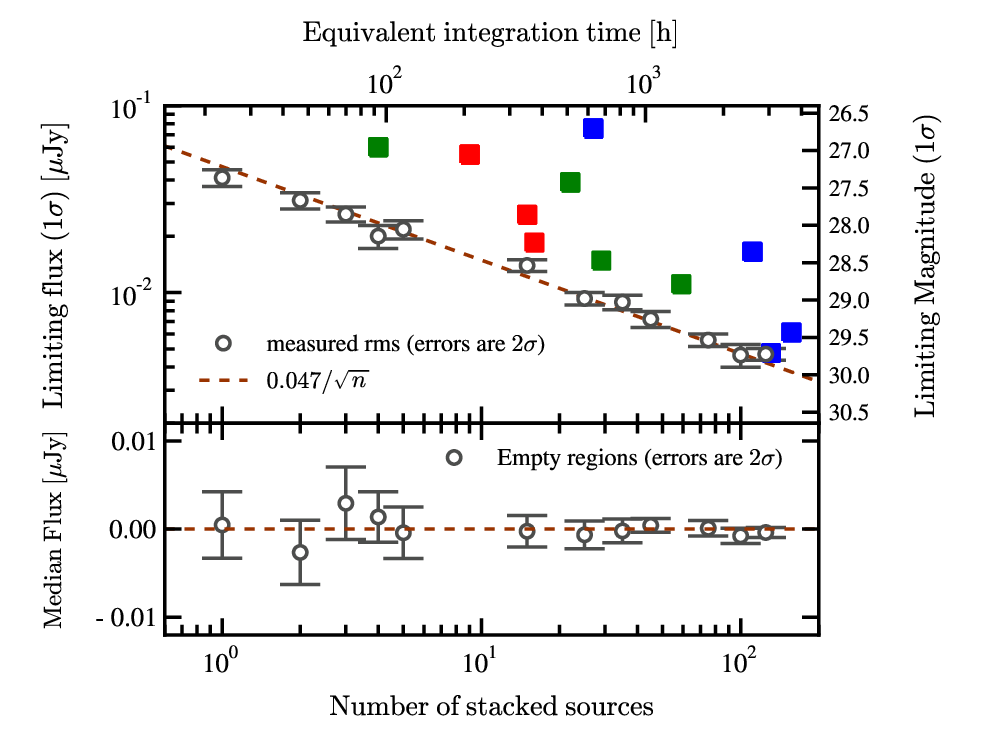
To estimate the uncertainty in the IRAC stacks, we also create bootstrap realizations. We treat the two epochs of IRAC data over the HUDF as independent stamps in the stack, thereby effectively weighting with exposure time, i.e., $N_{bin}=N_{ERS}+2N_{HUDF}$ . In each bootstrap draw, then, we draw with replacement $N_{ERS}+2N_{HUDF}$ such stamps, and estimate fluxes as described above. The image noise in each stacks is expected to decrease with the total equivalent exposure time approximately as $1/\sqrt{t_{exp,eq}}$ ( $t_{exp,eq}=(N_{ERS}+2N_{HUDF})\times 23.3\,$ hr). The actual photometric uncertainties that we derive are always greater than this because they also include the intrinsic scatter in the fluxes of the sources been stacked together (see Appendix). Stamps for all the IRAC median stacks along with the derived magnitudes and uncertainties are presented in Figures 2, 3, and 4. Table 2 is a compilation of all the stacked photometry including the Labbé et al. [27] stacks and information on the number of sources that go in each stack. It can be seen in the Figures that even for sources as faint as 27 mag, the stacks show good detections in both IRAC bands.

V. Rest-Frame UV-to-optical Colors of high- $z$ Star-Forming Galaxies.

The observed colors of galaxies can give us important information about the stellar populations that compose them. Usually, this is accomplished by comparing their colors with those of Synthetic Stellar Population (SSP) models. In this work, we chiefly explore the observed UV-to-optical colors and what can be learned from them and from their dependence on luminosity and redshift. When models are invoked, we use the Bruzual & Charlot [11, BC03] models and we assume a Salpeter [41] IMF, constant SFH, and $0.2\,Z_{\odot}$ metallicity, as these quantities cannot be constrained from our data. To derive best fits we use the SED fitting code FAST [25].

The rest-frame UV-to-optical color is of particular interest at high redshifts. Several studies have detected significant rest-frame UV-to-optical colors ( $\gtrsim 0.5\,$ mag) in $z\gtrsim 4$ galaxies [17, 16, 50, 45, 23, 22, 26, 27, 32]. The usual interpretation is that these colors derive from large Balmer breaks which are associated with evolved stellar populations with ages $\gtrsim 200\,$ Myr. This is surprising given how young the universe is at the time these galaxies are being observed. The main limitation for field studies is the depth of the $Spitzer$ /IRAC imaging available, which constrains these studies to the brightest LBGs. Searches behind clusters provide an alternative to probe the fainter populations (see, e.g., Ellis et al. 15, Bradley et al. 9, Richard et al. 39, Laporte et al. 29, and the recent tentative determination of a 1.5 mag Balmer break in a $z\sim 6$ galaxy by Richard et al. 38) but the number of sources amenable to such studies, remain low. We work around this limitation by stacking large numbers of sources which allows us to estimate the typical rest-frame UV-to-optical colors of faint $z\gtrsim 4$ sources.

We start by presenting the results found at $z\sim 4$ where the similar and complementary work of Lee et al. [30] allows us to study this colors over an unprecedentedly large range of UV-luminosities.

V.1. The UV-to-Optical Colors at $z\sim 4$ .

Our sample of $B-$ dropouts has a mean redshift of $\langle z\rangle=3.8\pm 0.3$ . We divide this sample based on their $i_{775}$ luminosity (which approximately corresponds to rest-frame 1500 Å) in four bins of $\Delta i_{775}=1$ mag. These are the same bins as shown in the histogram in Figure 1. The bins at $i_{775}>28$ mag are too faint to be detected in $Spitzer$ /IRAC and will not be included in the analysis. Assuming the mean redshift of the sample, these bins correspond approximately to $M_{1500}=-21,-20,-19,$ and $-18$ , which covers the moderately bright to faint end of the population ( $M^{*}_{1600,z=4}=-20.24$ , Bouwens et al. 5).

In a recent study, Lee et al. [30] focus on the median SEDs of the brightest $z\sim 4$ galaxies found in the ground based NOAO Deep Wide-Field Survey. Their sample has a mean redshift $\langle z\rangle=3.7\pm 0.4$ , and their SEDs also sample the rest-frame UV and optical using a combination of optical filters: $B_{W},\ R,\ I$ (Mosaic Camera), near-IR filters: $J,\ H,\ K_{s}$ (NEWFIRM Camera), and the $Spitzer$ /IRAC mid-IR channels 1 through 4¹¹ 1 Although relatively deep IRAC channels 3 & 4 data (sampling 5.8 $\mu$ m and 8.0 $\mu$ m respectively) is available for our sample in the GOODS-S, this data is still $\gtrsim 0.5\,$ mag shallower than the channel 1 & 2. It is, therefore, much harder to obtain reliable stacked photometry in those bands, especially considering that our sample is much smaller and intrinsically fainter than the Lee et al. [30] sample. We have not included these bands in the median-stacked SEDs presented in this work.. Similar to the present work, they divide their sample according to the $I$ –band luminosity, although with uneven bins. Their sources are intrinsically brighter than in this work, corresponding to $L>L^{*}_{z=4}$ sources roughly covering the range $-23\lesssim M_{1500}\lesssim-21$ .

The combination of the Lee et al. [30] sample with our data spans the UV-luminosity range: $-23\lesssim M_{1500}\lesssim-17.5$ . This represents an unprecedented dataset to study the SEDs, and especially the UV-to-optical colors, of $z\sim 4$ galaxies over a large range of luminosities. The SEDs from both works are presented in Figure 5. In this figure the $H_{160}$ is shown with open symbols since it is likely biased and should be ignored as is explained in detail later. An overall trend to bluer colors (both in the rest-frame UV and the rest-frame UV-to-optical colors) towards fainter luminosities is already apparent in this figure.

We quantify the UV-to-Optical colors by estimating the interpolated rest-frame $(U_{n}-V_{n})$ colors for the median-stacked SEDs in both sets. Figure 6 shows a not very steep but systematic trend of redder $(U_{n}-V_{n})_{rest}$ colors as a function of increasing UV-luminosity.

The interpolated $(U_{n}-V_{n})$ colors were determined from the best fits to the full observed SED, where the fits correspond to a linear combination of a set of template SEDs. These SEDs correspond to the default template set from the photometric code EAzY [10]. This template set was constructed and calibrated empirically to determine accurate photometric redshifts of galaxies of various types, from very blue starbursts to red ellipticals and has been shown to work well up to $z\sim 5-6$ [10]. For the $U_{n}$ and $V_{n}$ filters we have assumed narrow ideal filters that correspond to step functions of width 100 Å, centered at 3500 Å and 5500 Å for the $U_{n}$ and $V_{n}$ filters respectively. The colors were calculated from the best fit combination of templates using the filters described above. To estimate the uncertainty in the $(U_{n}-V_{n})_{rest}$ estimates, we perturbed the photometry and the redshift of each median-stacked SED within the allowed uncertainty, and a new fit was obtained. A new set of colors was measured from this best fit and the procedure was repeated a large number of times to derive the confidence intervals. A similar procedure was used to derive rest-frame $M_{1500}$ magnitudes for an ideal filter centered at 1500 Å and with a width of 100 Å.

For the data-point at $M_{1500}\sim-19$ , only an upper limit can be obtained due to the limitations of the template set used here. The EAzY default template set only includes SEDs with $(U_{n}-V_{n})_{rest}\gtrsim 0.3$ . The SED at $M_{1500}\sim-19$ is likely to have a $(U_{n}-V_{n})_{rest}$ color of $\sim 0.3\,$ mag, so no reliable lower limit can be obtained. We choose to show a $2\,\sigma$ upper limit. Other more sophisticated algorithms to determine interpolated rest-frame colors for an observed SED yield very similar results (e.g., the InterRest code, Taylor et al. 46, which implements the algorithm described in Rudnick et al. 40). However, such algorithms also depend on the template set resulting in similar limitations.

It is important to note that, when deriving this color from best fits, we have ignored the $H_{160}-$ band in our stacks and the $H$ and $K_{s}-$ bands in the Lee et al. [30] stacks. Given the redshift distribution of the sample it is expected that for some fraction of the sources (the ones at the lowest redshifts) the $H-$ band fluxes measured will include some rest-frame optical light. As a result, the estimated median rest-frame UV flux, will be biased towards larger values. To attempt a correction for this would require us knowing the exact redshift distribution of the sample, but even then a correction would be highly uncertain, so we opt to remove these photometric points from all fits.

In recent works, Bouwens et al. [4], Bouwens et al. [6] accurately determine the UV-slope of LBGs at $z>3$ as a function of UV-luminosity and redshift. For a star-forming stellar population, the UV-slope, parametrized by $\beta$ ( $f_{\lambda}\propto\lambda^{\beta}$ ), is most sensitive to the dust content of the galaxy. In consequence, the authors argue that the dependence of $\beta$ on UV-luminosity can be fully explained by an increase in the amount of dust that these galaxies contain as a they become brighter. If this is the case, a trend of redder $(U_{n}-V_{n})_{rest}$ colors for UV-brighter sources like the one observed here is also expected, since this color is also affected by dust extinction. The bottom panel of Figure 6 shows the $(U_{n}-V_{n})_{rest}$ colors corrected for dust extinction. These were derived as in Bouwens et al. [4], from the mean $\beta$ vs. UV-luminosity trend and the classic Meurer et al. [33] relation that relates the dust content with the UV-slope $\beta$ according to:

A_{1600}=4.43-1.99\beta

where $A_{1600}$ is the extinction in magnitudes at 1600 Å. A Calzetti et al. [13] extinction curve is used to estimate the extinction at other wavelengths.

Table 2Photometry Summary of Stacked SED.

Ref. mag	$N_{ERS}$	$N_{HUDF}$	$B_{435}$	$V_{606}$	$i_{775}$	$z_{850}$	$Y_{98}$	$Y_{105}$	$J_{125}$	$H_{160}$	$[3.6]$	$[4.5]$
$i_{775}$	$z\sim 4~B-$ dropouts
25	27 / 55	0 / 4	$27.5\pm 7.2$	$224.0\pm 14.9$	$363.2\pm 18.8$	$384.8\pm 24.7$	$366.5\pm 22.4$	$\cdots$	$405.5\pm 33.0$	$480.7\pm 53.4$	$784.5\pm 78.3$	$768.6\pm 117.2$
26	87 / 16	12 / 17	$13.5\pm 2.4$	$103.1\pm 3.8$	$150.1\pm 4.1$	$149.1\pm 5.8$	$146.8\pm 5.9$	$130.6\pm 8.9$	$147.9\pm 5.3$	$161.8\pm 7.1$	$268.8\pm 17.1$	$280.0\pm 17.6$
27	107 / 2	25 / 34	$8.4\pm 1.2$	$45.5\pm 1.7$	$58.9\pm 1.8$	$54.4\pm 2.4$	$55.0\pm 2.9$	$53.1\pm 3.2$	$56.1\pm 2.3$	$60.9\pm 3.4$	$83.8\pm 6.3$	$67.0\pm 7.5$
28	45 / 78	43 / 74	$3.6\pm 1.0$	$24.4\pm 1.0$	$27.2\pm 1.0$	$26.0\pm 1.6$	$29.4\pm 3.3$	$22.4\pm 1.5$	$26.8\pm 1.5$	$29.0\pm 2.1$	$41.4\pm 4.9$	$43.7\pm 7.2$
$z_{850}$	$z\sim 5~V-$ dropouts
25	4 / 9	0 / 0	$-6.2\pm 11.7$	$42.1\pm 8.1$	$227.4\pm 40.8$	$267.8\pm 21.8$	$273.0\pm 22.6$	$\cdots$	$281.9\pm 18.4$	$258.3\pm 19.3$	$681.9\pm 62.2$	$498.8\pm 59.9$
26	18 / 28	2 / 3	$0.9\pm 3.0$	$15.9\pm 3.7$	$104.7\pm 11.9$	$125.6\pm 8.1$	$114.5\pm 13.2$	$128.4\pm 17.4$	$126.3\pm 8.7$	$137.3\pm 11.1$	$337.9\pm 40.3$	$236.5\pm 41.5$
27	43 / 61	8 / 9	$-2.9\pm 2.1$	$8.3\pm 1.7$	$58.9\pm 4.2$	$63.9\pm 3.0$	$70.0\pm 5.6$	$62.1\pm 8.0$	$67.7\pm 3.9$	$63.0\pm 4.6$	$116.3\pm 11.5$	$89.4\pm 10.6$
28	11 / 24	9 / 13	$-0.8\pm 1.9$	$3.5\pm 1.4$	$24.5\pm 3.0$	$26.8\pm 2.6$	$25.5\pm 6.2$	$19.0\pm 3.7$	$25.9\pm 3.9$	$26.5\pm 3.9$	$58.0\pm 15.4$	$33.8\pm 15.7$
$Y$	$z\sim 6~i-$ dropouts
26	3 / 6	3 / 3	$1.2\pm 3.8$	$-1.5\pm 3.6$	$12.1\pm 6.6$	$93.0\pm 14.7$	$102.2\pm 12.1$	$143.2\pm 23.8$	$116.4\pm 14.8$	$133.6\pm 26.3$	$278.7\pm 56.8$	$187.7\pm 42.1$
27	11 / 17	2 / 3	$-0.5\pm 3.4$	$0.1\pm 2.4$	$14.2\pm 5.0$	$64.5\pm 6.5$	$60.2\pm 7.4$	$48.7\pm 5.1$	$64.2\pm 5.9$	$68.4\pm 7.8$	$142.2\pm 27.0$	$111.9\pm 31.8$
28	4 / 4	6 / 13	$-2.5\pm 2.5$	$0.5\pm 2.1$	$-0.7\pm 3.6$	$30.3\pm 5.4$	$30.7\pm 8.9$	$24.6\pm 3.4$	$33.0\pm 5.8$	$26.2\pm 6.3$	$61.3\pm 19.2$	$39.9\pm 20.0$
$H_{160}$	$z\sim 7~z-$ dropouts
26	$\cdots$	$\cdots$	$-3.2\pm 2.3$	$2.8\pm 2.3$	$-7.4\pm 4.7$	$23.5\pm 5.4$	$63.7\pm 7.7$	$\cdots$	$129.7\pm 16.0$	$128.2\pm 17.0$	$262.0\pm 28.0$	$181.0\pm 37.0$
27	$\cdots$	$\cdots$	$-2.4\pm 0.8$	$-0.8\pm 0.6$	$2.2\pm 1.8$	$14.6\pm 2.3$	$49.1\pm 4.3$	$\cdots$	$64.8\pm 4.1$	$57.0\pm 3.4$	$107.0\pm 16.0$	$83.8\pm 25.0$
28	$\cdots$	$\cdots$	$1.2\pm 0.8$	$0.4\pm 0.5$	$-0.1\pm 0.7$	$5.6\pm 1.1$	$27.2\pm 1.8$	$\cdots$	$29.6\pm 2.0$	$24.5\pm 1.6$	$45.1\pm 9.5$	$39.3\pm 17.0$

Note. — The median SEDs of high $-z$ galaxies in bins of observed UV-luminosity. The fluxes are in units of nJy. $N_{HUDF}$ and $N_{ERS}$ are the numbers of sources with reliable IRAC photometry over the total available in the given bin. Only the ones with reliable photometry were considered in the stack. The $z\sim 7$ stacks were taken directly from Labbé et al. [27].

As can be seen from the figure, the dust corrected $(U_{n}-V_{n})$ color is essentially constant with UV-luminosity. This again suggests that the main origin for the correlation of $\beta$ with the UV-luminosity is an increasing dust content at brighter magnitudes. Otherwise we would expect some residual trend in the dust corrected color. This would be the case for example, if a strong age trend existed with UV-luminosity. As will be shown later, a similar flattening of the corrected colors is observed at all redshifts in the $-21<M_{1500}<-18$ range.

Although both are flat, the trends of the corrected colors with UV-luminosity of the two samples are disjoint. The reasons for this are unclear but there are a couple of reasons that may help explain it. First, it is unclear that the mean trend used to derive dust corrections applies over such a large range of luminosities. This can help to explain that the corrected colors of the brightest sources are bluer than those of the faintest ones. However, it does not explain the break between the two samples. Second there are differences between the selection of the two samples, in particular, it is not clear that the fraction of contaminants is comparable between the two samples. A larger fraction of contaminants in the brighter ground-based sample of Lee et al. [30] as compared to the our data, could bias the brighter SEDs to smaller $(U_{n}-V_{n})$ colors, resulting in excessive corrections for dust, which are derived from the mean trend on the UV with UV-luminosity. It should also be noted that in the case of the Lee et al. [30] sample, the UV-slope is not very well sampled, with basically the $I$ and $J-$ bands driving the UV-slope (since the $H-$ band has been excluded). Even small systematic offsets of $\sim 0.1\,$ mag in the zero-point calibration between these two filters can bias the best fit models to redder slopes and in consequence, smaller UV-to-optical colors.

V.2. The UV-to-optical Colors at Higher Redshift

Table 3Rest Frame Magnitude and Colors.

$M_{1500}$	$J_{125}-[3.6]$	$(U-V)_{rest}$	$(U-V)_{dust-corr}$
$z\sim 4~B-$ dropouts
$-20.87\pm 0.23$	$0.71\pm 0.14$	$0.57\pm 0.10$	$0.38$
$-19.90\pm 0.19$	$0.65\pm 0.08$	$0.47\pm 0.06$	$0.33$
$-18.86\pm 0.17$	$0.44\pm 0.09$	$>0.49$	$>0.41$
$-17.99\pm 0.15$	$0.45\pm 0.15$	$0.39\pm 0.06$	$0.36$
$z\sim 5~V-$ dropouts
$-21.03\pm 0.14$	$0.96\pm 0.12$	$0.58\pm 0.06$	$0.40$
$-20.18\pm 0.14$	$1.07\pm 0.15$	$0.61\pm 0.07$	$0.47$
$-19.51\pm 0.13$	$0.60\pm 0.13$	$0.37\pm 0.05$	$0.27$
$-18.43\pm 0.18$	$0.87\pm 0.33$	$0.50\pm 0.14$	$0.46$
$z\sim 6~i-$ dropouts
$-20.35\pm 0.20$	$0.93\pm 0.28$	$0.50\pm 0.12$	$0.44$
$-19.64\pm 0.12$	$0.88\pm 0.23$	$0.58\pm 0.11$	$0.56$
$-18.79\pm 0.15$	$0.70\pm 0.41$	$0.48\pm 0.15$	$0.50$
$z\sim 7~z-$ dropouts
$-20.73\pm 0.22$	$0.76\pm 0.18$	$0.48\pm 0.12$	$0.35$
$-19.93\pm 0.12$	$0.54\pm 0.18$	$0.45\pm 0.12$	$0.40$
$-19.08\pm 0.13$	$0.44\pm 0.23$	$0.44\pm 0.14$	$0.48$

Note. — Rest frame $M_{1500}$ estimated from the best fit power-law to the rest-frame UV photometry. Possibly contaminated bands were ignored in the fit (see open points in Figure 7).

We now extend our determination of the SED of high- $z$ galaxies to $z\sim 5$ and $z\sim 6$ , and combine our determinations with the stacked SEDs of sources at $z\sim 7$ recently presented in Labbé et al. [27]. Figure 7 shows the SEDs at $4\lesssim z\lesssim 7$ . The expected mean redshifts of these samples correspond to $\langle z\rangle=3.8,\langle z\rangle=5.0,\langle z\rangle=5.9,$ and $\langle z\rangle=6.9$ , with typical spread in redshift of $\Delta z\pm 0.3$ . The samples at each redshift have been split in bins of 1 mag, using as reference the observed magnitude in the band closest to 1500 Å (Table 2 contains the SEDs and information about the samples in each bin). Best fit BC03 models with CSF and $0.2Z_{\odot}$ metallicity are overlaid for reference. As explained in the previous section, we have excluded from the fitting the bands that are potentially biased (marked by the open symbols). As can be seen in this Figure, all these SEDs are remarkably similar and show sizable UV-to-optical colors.

The similarity of the SEDs can also be appreciated in Figure 8, where the SEDs from the different redshift samples have been grouped according to their approximate $M_{1500}$ luminosities. The SEDs in the three $M_{1500}$ bins have been re-normalized according to their $M_{1500}$ luminosity and combined to produce over-sampled SEDs, which take advantage of the fact that the different filters probe different rest-frame wavelengths at the different redshifts. The combined SEDs show the typical flat UV slopes, but also rather flat colors in the rest-frame optical, albeit with a relatively large scatter. This scatter can in part be a consequence of the normalization which is done in the far UV, which effectively acts as the pivot point. Different emission lines that sometimes contribute flux in the IRAC bands, depending on the redshift, can also be contributing to this scatter.

V.2.1 Emission lines in the rest-frame optical.

We first consider the implications if the sizable red $J_{125}-[3.6]$ colors that we observe are assumed to be exclusively measuring the stellar continuum in these high redshift galaxies. The red color would arise from large Balmer breaks, and would be indicative of evolved stellar populations. As can be seen in Figure 9a, the $J_{125}-[3.6]$ colors characteristic of these sources would then require fairly large ages of $\sim 1$ Gyr if no dust is allowed in the models (the model tracks in the Figure are CSF models). Allowing some reddening by dust (using in this case a Calzetti et al. 13 law), reduces their ages considerably (Figure 9c). The amount of dust reddening is constrained however. Based on the UV continuum slopes typically observed in these galaxies [4], and using the $z=0$ Meurer et al. [33] relation between this slope and the dust content, it has been shown that the reddening at $z\gtrsim 4$ is typically $A_{V}\lesssim 0.7\,$ mag. The reddening is likely to be even smaller at higher redshifts [4, 6]. With this added constraint, the ages derived from SED fitting are generally estimated to be $300-400$ Myr [50, 17, 45, 23, 27, e.g.,].

In our SEDs at $z\gtrsim 5$ we also find that the $([3.6]-[4.5])$ color is consistently blue, with typical values of $\sim-0.3\,$ mags. This color is very hard to reproduce with a model with any star formation history that is based only on stellar continuum. The addition of dust only makes the comparison worse (Figure 9c,d). It should be noted, however, that the uncertainties in this color are considerable and that in most cases the observed color is formally consistent with the stellar continuum only models.

It has been claimed [42, 43] that at some of these redshifts, particularly $z\sim 6$ and 7, the SEDs could be better fit by very young stellar population models ( $\lesssim 10$ Myr old) with moderate dust content and very strong nebular emission lines. These lines would dominate the rest-frame optical fluxes. As the galaxies are forming stars, it is likely that they have nebular emission lines, and so we have assessed whether emission lines could be influencing our fluxes and fits. The observed position of the most prominent optical nebular emission lines at each redshift is marked in Figure 7 by the dashed vertical lines (assuming the mean redshift of each sample). It can be seen that at the different redshifts involved, some of the rest-frame optical emission lines would lie within the IRAC [3.6] and [4.5] filters.

Atek et al. [2] showed recently that at $z<2.8$ there are sources that show emission lines with large enough equivalent widths to dominate the broadband fluxes in the optical. However, even for their sample of high equivalent width selected sources, such objects are not very common. For the more typical cases, the lines that they find in their sample would have moderate contributions to the IRAC broad bands, usually making them $0.2-0.3\,$ mags brighter. At higher redshifts, $3.8\lesssim z\lesssim 5$ , the work of Shim et al. [44], based on spectroscopic redshifts and IRAC broadband photometry, finds similar results. They find that the sources in this redshift range show an excess of flux in [3.6] over [4.5], which the authors think can be explained by H $\alpha$ emission. The majority of the sources in their sample have $([3.6]-[4.5])$ colors that are consistent with an H $\alpha$ contribution of $0.2-0.3\,$ mags to the [3.6] filter, indicating moderate contributions from emission lines.

We consider the effects of a similar (moderate) contribution of emission lines to the colors of a 280 Myr old CSF model. For the purpose of this exercise we assume a H $\alpha$ rest-frame equivalent width ${\rm EW_{rest}}=300\,$ Å. At $z\sim 6$ , this would increase the luminosity in the [4.5] filter by 0.23 mag. We only consider the strongest lines in the optical and assume the strength ratios presented by Anders & Fritze-v. Alvensleben [1] for a $0.2\,{\rm Z_{\odot}}$ metallicity system. This corresponds to ${\rm EW_{rest}(OII,H\beta,OIII)=(189,105,670)\,}$ Å, respectively. The open squares in Figure 9a,b, correspond to the median colors for a model like the one described (the median takes into account the expected redshift distribution of each sample).

As can be seen in Figure 9a, the main effect of the contribution from the emission lines is that it allows for significantly younger ages to reproduce the $J_{125}-[3.6]$ colors (by roughly a factor of two). Since this implies lower stellar continuum fluxes than previously assumed, this would also result in lower best fit stellar masses than previously estimated for galaxies at these redshifts (by a similar factor). Simultaneously, given the line ratios and the redshift distributions expected for these samples, a model like this can also help in reproducing the blue [3.6]-[4.5] colors of the SEDs at $z\gtrsim 5$ (Figure 9b). While formally models with just stellar continua can fit the data, given the current large uncertainties, such colors are hard to obtain with stellar continuum only models. It is more likely that some degree of contribution of emission lines provides a better solution.

The assessment presented here is necessarily very simplistic, given the current uncertainties, and is only meant to show the possible effects of emission lines on the colors of these galaxies. Better estimates of the contribution of these lines and its effects on the properties derived from SED fitting will depend on the actual strengths and ratios of the lines. Moderate improvement can be achieved if more precise redshifts are known for these sources, such data does not exist at this time for such faint high redshift galaxies and so this remains an open question until improved spectroscopic capability becomes available.

V.2.2 UV-to-optical color vs. luminosity.

Regarding the trend of redder UV-to-optical colors for brighter UV-luminosities presented in Figure 6 for the $z\sim 4$ sample, it can also be observed for the other samples. In fact, within the uncertainties in the color determination, the $J_{125}-[3.6]$ vs $M_{1500}$ trend is roughly the same at $z\sim 5$ and 6 (Figure 10, top). This is particularly remarkable in view of the fact that this color is an observed color, not a rest-frame color, and in consequence is probing different wavelengths for the different samples. This shows again how similar and flat these SEDs are. If all the SEDs are considered simultaneously, a trend of $J_{125}-[3.6]=-0.12(\pm 0.07)\times M_{1500,AB}+const$ , is found. For simple CSF models, this trend implies a variation in stellar M/L ratio. González et al. [22] find that at $z\sim 4$ , this variation is of a factor $\sim\times 5$ between $M_{1500}=-18$ and $M_{1500}=-21$ . So, despite the steep UV-luminosity functions characteristic at $z\gtrsim 4$ , the contribution of the faintest sources to the total stellar mass density is more modest than their contribution to the star formation rate density.

Similar to the analysis performed at $z\sim 4$ , we have derived rest-frame $(U_{n}-V_{n})$ colors for the median SEDs at all redshifts. These colors are shown in Figure 10. The trend with UV-luminosity has large scatter and low significance but is systematic in the sense that brighter sources are redder in $(U_{n}-V_{n})_{rest}$ . A fit to the rest-frame colors as a function of M₁₅₀₀ of all redshifts simultaneously, results in $(U_{n}-V_{n})=-0.04\times M_{1500}-0.37$ , shown as the brown dashed line in Figure 10 (center panel). This is slightly steeper than the $-0.03$ slope found for the $z\sim 4$ data only, also plotted for reference as the black dashed line in the same Figure. The latter trend included the bright sample of Lee et al. [30] and is consistent within the uncertainties with the fit to all the points.

Using the median trends determined by Bouwens et al. [6] regarding the $\beta$ slopes vs. UV-luminosity for $4\lesssim z\lesssim 7$ LBGs, we corrected the $(U-V)_{rest}$ colors for dust extinction using the Meurer et al. [33] relation (Figure 10, bottom). These corrected colors show large scatter around $(U-V)_{rest,corrected}\sim 0.4$ but there is no indication of a residual trend with UV-luminosity except for the $z\sim 7$ sample (black symbols). This may indicate again that at $4\lesssim z\lesssim 6$ , the evolution can be fully explained by a change in dust content and there is no strong evolution in the ages of these sources as a function of UV-luminosity. This is consistent with the report by [45] based on stellar population modeling of slightly brighter LBGs in this redshift range. It is also consistent with the predictions from the hydrodynamical simulations of Finlator et al. [20], which find no trend of age with UV-luminosity.

At $z\sim 7$ there seems to be a residual trend in $(U_{n}-V_{n})_{rest,corrected}\sim 0.4$ vs. UV-luminosity in the sense that brighter sources have systematically bluer intrinsic $(U_{n}-V_{n})$ colors. In principle, this could indicate that the brighter sources are actually younger than the fainter sources, which would be difficult to imagine. Alternatively, it is possible that the simple dust corrections (calibrated at $z=0$ ) are not adequate at these high redshifts, due to, for example, changes in the IMF, metallicity, or escape fraction, all of which could alter the UV-slope $\beta$ for a given dust content. It should also be noted that the $\beta$ vs. UV-luminosity at $z\sim 7$ is considerably steeper than at the other redshifts and so the corrections to the $(U_{n}-V_{n})_{rest}$ vs. UV-luminosity trend are more extreme. Nevertheless, the uncertainties are sufficiently large that also the $z\sim 7$ trend is fully consistent with being constant.

VI. Summary

Determining the rest-frame UV-to-optical colors of individual UV-faint galaxies at $z\gtrsim 4$ is challenging. At such redshifts the rest-frame optical lies at $\lambda>2.5$ microns in the mid-IR and so it is hard to measure at the extremely faint magnitudes typical of galaxies in the first 1.5 Gyr. To gain insight into the typical spectral properties of $z\sim 4-6$ galaxies, we have taken advantage of the large samples of $z\sim 4-6$ sources found in the deep HST ACS and WFC3/IR images of the ERS and HUDF fields. The HST data give us rest-frame UV fluxes. We then use $Spitzer$ /IRAC [3.6] and [4.5] micron data from the deep GOODS survey of these fields to get rest-frame optical fluxes by stacking the IRAC images and determining median flux values. This allows us to determine the SEDs of these galaxies covering both the rest-frame UV and the optical. These SEDs represent a first comprehensive study of the rest-frame UV-to-optical properties of $z\gtrsim 4$ galaxies as a function of both redshift and UV-luminosity down to very faint limits.

At $z\gtrsim 4$ we have also combined our faint SEDs with the $L>L^{*}$ stacks presented in Lee et al. [30]. This allows us to assess the colors of $z\gtrsim 4$ sources over an unprecedentedly large range of luminosities. Our main findings are as follow:

•

At $z\gtrsim 4$ the $(U_{n}-V_{n})$ rest-frame color (interpolated from the data using a fitted SED from a set of templates is of $(U_{n}-V_{n})\sim 0.5\,$ mags. There is a shallow but systematic trend of redder colors for brighter UV-luminosities over the range $-23\lesssim M_{1500,AB}\lesssim-17.5$ (Figure 6, section 5.1). A linear fit to this trend is $(U_{n}-V_{n})_{rest}=-0.03\times$ M ${}_{1500}-0.07$
•

The SEDs of star forming galaxies at $4\lesssim z\lesssim 7$ are remarkably similar at all luminosities from $-23\lesssim M_{1500,AB}\lesssim-17.5$ , showing fairly flat rest-frame UV and rest-frame optical colors (section 5.2 and Figures 7, 8 and 10). At a given redshift, there are weak indications of a subtle trend for redder colors for brighter sources. A simple fit to the data at all redshifts simultaneously results in $(U_{n}-V_{n})_{rest}=-0.04\times$ M ${}_{1500}-0.37$ (Figure 10 center, Section 4.2).
•

The UV-to-optical color, as measured by the observed $J_{125}-[3.6]$ , color remains fairly constant with redshift, despite the $Spitzer$ /IRAC bands probing different wavelength regions of the SED (Figure 10 top). This suggests that the optical colors are fairly flat at all redshifts $z\sim 4-7$ , although there is significant scatter, which can be caused by optical emission line contamination to the IRAC filters.
•

The $z\gtrsim 5$ SEDs show consistently blue $[3.6]-[4.5]\sim-0.3$ colors. This is hard to reproduce with models that only include stellar continuum, although it is still formally possible given the current uncertainties. Nonetheless, it is probably better explained with moderate flux contributions from optical nebular emission lines in the two IRAC bands. Including some contribution from emission lines leads to lower best fit ages and lower stellar masses than previously estimated for galaxies at these redshifts. Changes of a factor 2 could well result, but we would caution that detailed assessments are not yet possible with the current data.
•

We derive dust-corrected $(U-V)$ colors using a simple dust correction based on the median UV-slope $\beta$ vs. UV-luminosity relation from Bouwens et al. [4], Bouwens et al. [6] and the Meurer et al. [33] relation (Figure 10, bottom). The dust-corrected UV-to-optical colors at $4\lesssim z\lesssim 6$ are $(U-V)\sim 0.4\,$ mags. They do not appear to depend on UV-luminosity. This may suggest that moderate changes in the dust content of galaxies can explain the color dependency observed both in the UV-slopes and the UV-to-optical colors. In particular, it seems that no age evolution is required to match this color dependency.

The recent deep and ultra-deep HST ACS and WFC3/IR imaging programs over the GOODS-S field have resulted in large samples of $z\sim 4$ galaxies. Taking advantage of these large samples, along with a careful stacking analysis, we present a first comprehensive study of the typical SEDs over the rest-frame UV and the rest-frame optical for faint star forming galaxies in the $4\lesssim z\lesssim 7$ redshift range. The stacked SEDs allow us to study the UV-to-optical colors of high-z star forming galaxies down to very low luminosities. We find a weak trend to bluer color at fainter luminosities. Interestingly, these stacked SEDs also show a remarkable similarity across redshift in a period of considerable stellar mass growth from about 0.8 Gyr to 1.5 Gyr, suggesting a smooth self-similar mode of evolution at $z\sim 7-4$ .

We acknowledge support from NASA grant HST-GO-11563, and NASA grant HST-GO-11144. This work is based on observations made with the Hubble Space Telescope and with the Spitzer Space Telescope. Support for this work was provided by NASA through an award issued by JPL/Caltech. P.O. acknowledges support provided by NASA through Hubble Fellowship grant HF-51278.01 awarded by the Space Telescope Science Institute, which is operated by the Association of Universities for Research in Astronomy, Inc., for NASA, under contract NAS 5- 26555.

References

[1] Anders, P., & Fritze-v. Alvensleben, U. 2003, A&A, 401, 1063
[2] Atek, H., et al. 2011, arXiv:1109.0639
[3] Bertin, E., & Arnouts, S. 1996, A&AS, 117, 393
[4] Bouwens, R. J., et al. 2009, ApJ, 705, 936
[5] Bouwens, R. J., Illingworth, G. D., Franx, M., & Ford, H. 2007, ApJ, 670, 928
[6] Bouwens, R. J., et al. 2011, arXiv:1109.0994
[7] —. 2010a, ApJ, submitted, arXiv:1006.4360
[8] —. 2010b, ApJ, 709, L133
[9] Bradley, L. D., et al. 2008, ApJ, 678, 647
[10] Brammer, G. B., van Dokkum, P. G., & Coppi, P. 2008, ApJ, 686, 1503
[11] Bruzual, G., & Charlot, S. 2003, MNRAS, 344, 1000
[12] Bunker, A. J., et al. 2010, MNRAS, 409, 855
[13] Calzetti, D., Armus, L., Bohlin, R. C., Kinney, A. L., Koornneef, J., & Storchi-Bergmann, T. 2000, ApJ, 533, 682
[14] Dunlop, J. S., McLure, R. J., Robertson, B. E., Ellis, R. S., Stark, D. P., Cirasuolo, M., & de Ravel, L. 2011, arXiv:1102.5005
[15] Ellis, R., Santos, M. R., Kneib, J.-P., & Kuijken, K. 2001, ApJ, 560, L119
[16] Eyles, L. P., Bunker, A. J., Ellis, R. S., Lacy, M., Stanway, E. R., Stark, D. P., & Chiu, K. 2007, MNRAS, 374, 910
[17] Eyles, L. P., Bunker, A. J., Stanway, E. R., Lacy, M., Ellis, R. S., & Doherty, M. 2005, MNRAS, 364, 443
[18] Finkelstein, S. L., Papovich, C., Giavalisco, M., Reddy, N. A., Ferguson, H. C., Koekemoer, A. M., & Dickinson, M. 2010, ApJ, 719, 1250
[19] Finkelstein, S. L., et al. 2011, arXiv:1110.3785
[20] Finlator, K., Oppenheimer, B. D., & Davé, R. 2011, MNRAS, 410, 1703
[21] Giavalisco, M., et al. 2004, ApJ, 600, L93
[22] González, V., Labbé, I., Bouwens, R. J., Illingworth, G., Franx, M., & Kriek, M. 2011, ApJ, 735, L34+
[23] González, V., Labbé, I., Bouwens, R. J., Illingworth, G., Franx, M., Kriek, M., & Brammer, G. B. 2010, ApJ, 713, 115
[24] Khochfar, S., & Silk, J. 2011, MNRAS, 410, L42
[25] Kriek, M., van Dokkum, P. G., Labbé, I., Franx, M., Illingworth, G. D., Marchesini, D., & Quadri, R. F. 2009, ApJ, 700, 221
[26] Labbé, I., Bouwens, R., Illingworth, G. D., & Franx, M. 2006, ApJ, 649, L67
[27] Labbé, I., et al. 2010a, ApJ, 716, L103
[28] —. 2010b, ApJ, 708, L26
[29] Laporte, N., et al. 2011, A&A, 531, A74+
[30] Lee, K.-S., et al. 2011, ApJ, 733, 99
[31] McLure, R. J., Dunlop, J. S., Cirasuolo, M., Koekemoer, A. M., Sabbi, E., Stark, D. P., Targett, T. A., & Ellis, R. S. 2010, MNRAS, 403, 960
[32] McLure, R. J., et al. 2011, arXiv:1102.4881
[33] Meurer, G. R., Heckman, T. M., & Calzetti, D. 1999, ApJ, 521, 64
[34] Noeske, K. G., et al. 2007, ApJ, 660, L43
[35] Oesch, P. A., et al. 2010, ApJ, 709, L16
[36] —. 2011, arXiv:1105.2297
[37] Oke, J. B., & Gunn, J. E. 1983, ApJ, 266, 713
[38] Richard, J., Kneib, J.-P., Ebeling, H., Stark, D. P., Egami, E., & Fiedler, A. K. 2011, MNRAS, 414, L31
[39] Richard, J., Stark, D. P., Ellis, R. S., George, M. R., Egami, E., Kneib, J.-P., & Smith, G. P. 2008, ApJ, 685, 705
[40] Rudnick, G., et al. 2003, ApJ, 599, 847
[41] Salpeter, E. E. 1955, ApJ, 121, 161
[42] Schaerer, D., & de Barros, S. 2009, A&A, 502, 423
[43] —. 2010, A&A, 515, A73+
[44] Shim, H., Chary, R.-R., Dickinson, M., Lin, L., Spinrad, H., Stern, D., & Yan, C.-H. 2011, arXiv:1103.4124
[45] Stark, D. P., Ellis, R. S., Bunker, A., Bundy, K., Targett, T., Benson, A., & Lacy, M. 2009, ApJ, 697, 1493
[46] Taylor, E. N., et al. 2009, ApJS, 183, 295
[47] Weinmann, S. M., Neistein, E., & Dekel, A. 2011, arXiv:1103.3011
[48] Wilkins, S. M., Bunker, A. J., Stanway, E., Lorenzoni, S., & Caruana, J. 2011, MNRAS, 1340
[49] Yan, H., Dickinson, M., Giavalisco, M., Stern, D., Eisenhardt, P. R. M., & Ferguson, H. C. 2006, ApJ, 651, 24
[50] Yan, H., et al. 2005, ApJ, 634, 109
[51] Yan, H., Windhorst, R. A., Hathi, N. P., Cohen, S. H., Ryan, R. E., O’Connell, R. W., & McCarthy, P. J. 2010, Research in Astronomy and Astrophysics, 10, 867

Appendix A A. Depth of the Stacks

To quantify the rest-frame optical properties of very faint high-redshift galaxies, we stack the IRAC images for a large number of faint galaxies, after removing the flux contribution from nearby neighbors (section 4). While we do not expect large systematics in the photometry of individual sources from our deblending procedure to remove neighboring sources, it is possible that modest systematics could arise when stacking a large number of sources. The role of this appendix is to determine how large such systematics might be. Fortunately we are able to demonstrate that the fluxes that we measure in the stacked IRAC images are unbiased and that their significance is properly determined.

We started by selecting 200 empty areas in the HUDF field. We select them based on the segmentation maps derived from the high resolution HST images. We processed each of the selected empty areas as if they were the position of one of the real sources in our catalog, i.e. we ran them through the de-blending code to remove the flux from nearby un-associated sources. To determine the rms for a given $N_{stacked}$ number of stacked stamps, we randomly draw (with replacement) $N_{stacked}$ stamps from the 200 empty areas, median combine them and perform aperture photometry in the median stack in the same fashion as for our real stacks. We repeat the drawing 300 times and measure the rms of these 300 trials. As can be seen in the upper panel of Figure 11, the limiting flux decreases as $\propto 1/\sqrt{N_{stacked}}$ , as expected for background-limited noise. In the case of the stacks that contain real sources, the rms is larger than the image noise because it is also affected by the intrinsic variation in the distribution of fluxes that are being stacked.

As can be seen in the lower panel, the flux of the median stacks is very close to the expected zero flux.

The Rest Frame UV to Optical Colors and SEDs of z∼4−7z\sim 4-7 galaxies.