Jones polynomials, volume and essential knot surfaces: A surveyThanks: D.F. is supported in part by NSF grant DMS–1007221.Thanks: E.K. is supported in part by NSF grants DMS–0805942 and DMS–1105843.Thanks: J.P. is supported in part by NSF grant DMS–1007437 and a Sloan Research Fellowship.Thanks:  August 24, 2026

Associated to a diagram $D$ and a crossing $x$ of $D$ are two link diagrams, each with one fewer crossing than $D$. These are obtained by removing the crossing $x$, and reconnecting the diagram in one of two ways, called the $A$–resolution and $B$–resolution of the crossing, shown in Figure 1.

For each crossing of $D$, we may make a choice of $A$–resolution or $B$–resolution, and end up with a crossing–free diagram. Such a choice of $A$– or $B$–resolutions is called a Kauffman state, denoted $\sigma$. The resulting crossing–free diagram is denoted by $s_{\sigma}$.

The first graph associated with our diagram will be trivalent. We start with the crossing–free diagram given by a state. The components of this diagram are called state circles. For each crossing $x$ of $D$, attach an edge from the state circle on one side of the crossing to the other, as in the dashed lines of Figure 1. Denote the resulting graph by $H_{\sigma}$. Edges of $H_{\sigma}$ come from state circles and crossings; there are two trivalent vertices for each crossing.

To obtain the second graph, collapse each state circle of $H_{\sigma}$ to a vertex. Denote the result by ${\mathbb{G}}_{\sigma}$. The vertices of ${\mathbb{G}}_{\sigma}$ corespond to state circles, and the edges correspond to crossings of $D$. The graph ${\mathbb{G}}_{\sigma}$ is called the state graph associated to $\sigma$.

In the special case where each state circle of $\sigma$ traces a region of the diagram $D(K)$, the state graph ${\mathbb{G}}_{\sigma}$ is called a checkerboard graph or Tait graph. These checkerboard graphs record the adjacency pattern of regions of the diagram, and have been studied since the work of Tait and Listing in the 19th century. See e.g. [38, Page 264].

Our primary focus from here on will be on the all–$A$ state, which consists of choosing the $A$–resolution at each crossing, and similarly the all–$B$ state. Their corresponding state graphs are denoted ${\mathbb{G}}_{A}$ and ${\mathbb{G}}_{B}$. An example of a diagram, as well as the graphs $H_{A}$ and ${\mathbb{G}_{A}}$ that result from the all–$A$ state, is shown in Figure 2.

For the all–$A$ and all–$B$ states, we define graphs ${\mathbb{G}^{\prime}_{A}}$ and ${\mathbb{G}^{\prime}_{B}}$ by removing all duplicate edges between pairs of vertices of ${\mathbb{G}}_{A}$ and ${\mathbb{G}}_{B}$, respectively. Again see Figure 2.

The following definition, formulated by Lickorish and Thistlethwaite [31, 41], captures the class of link diagrams whose Jones polynomial invariants are especially well–behaved.

We will devote most of our attention to $A$–adequate knots and links. Because the mirror image of a $B$–adequate knot is $A$–adequate, this includes the $B$–adequate knots up to reflection. We remark that the class of $A$– or $B$–adequate links is large. It includes all prime knots with up to 10 crossings, alternating links, positive and negative closed braids, closed 3–braids, Montesinos links, and planar cables of all the above [31, 40, 41]. In fact, Stoimenow has computed that there are only two knots of 11 crossings and a handful of 12 crossing knots that are not $A$– or $B$–adequate. Furthermore, among the 253,293 prime knots with 15 crossings tabulated in Knotscape [24], at least 249,649 are either $A$–adequate or $B$–adequate [40].

Recall that a link diagram $D$ is called prime if any simple closed curve that meets the diagram transversely in two points bounds a region of the projection plane without any crossings. A prime knot or link admits a prime diagram.

Here, we recall a topological construction that allows us to recover the Jones polynomial of any knot or link from a certain $2$–dimensional embedding of ${\mathbb{G}_{A}}$.

A connected link diagram $D$ leads to the construction of a Turaev surface [44], as follows. Let $\Gamma\subset S^{2}$ be the planar, 4–valent graph of the link diagram. Thicken the (compactified) projection plane to a slab $S^{2}\times[-1,1]$, so that $\Gamma$ lies in $S^{2}\times\{0\}$. Outside a neighborhood of the vertices (crossings), our surface will intersect this slab in $\Gamma\times[-1,1]$. In the neighborhood of each vertex, we insert a saddle, positioned so that the boundary circles on $S^{2}\times\{1\}$ are the components of the $A$–resolution $s_{A}(D)$, and the boundary circles on $S^{2}\times\{-1\}$ are the components of $s_{B}(D)$. (See Figure 3.) Then, we cap off each circle with a disk, obtaining an unknotted closed surface $F(D)$.

In the special case when $D$ is an alternating diagram, each circle of $s_{A}(D)$ or $s_{B}(D)$ follows the boundary of a region in the projection plane. Thus, for alternating diagrams, the surface $F(D)$ is exactly the projection sphere $S^{2}$. For general diagrams, it is still the case that the knot or link has an alternating projection to $F(D)$ [8, Lemma 4.4].

The construction of the Turaev surface $F(D)$ endows it with a natural cellulation, whose $1$–skeleton is the graph $\Gamma$ and whose $2$–cells correspond to circles of $s_{A}(D)$ or $s_{B}(D)$, hence to vertices of ${\mathbb{G}_{A}}$ or ${\mathbb{G}_{B}}$. These $2$–cells admit a natural checkerboard coloring, in which the regions corresponding to the vertices of ${\mathbb{G}_{A}}$ are white and the regions corresponding to ${\mathbb{G}_{B}}$ are shaded. The graph ${\mathbb{G}_{A}}$ (resp. ${\mathbb{G}_{B}}$) can be embedded in $F(D)$ as the adjacency graph of white (resp. shaded) regions. Note that the faces of ${\mathbb{G}_{A}}$ (that is, regions in the complement of ${\mathbb{G}_{A}}$) correspond to vertices of ${\mathbb{G}_{B}}$, and vice versa. In other words, the graphs are dual to one another on $F(D)$.

A graph, together with an embedding into an orientable surface, is often called a ribbon graph. Ribbon graphs and their polynomial invariants have been studied by many authors, including Bollobas and Riordan [4, 5]. Building on this point of view, Dasbach, Futer, Kalfagianni, Lin and Stoltzfus [8] showed that the ribbon graph embedding of ${\mathbb{G}_{A}}$ into the Turaev surface $F(D)$ carries at least as much information as the Jones polynomial $J_{K}(t)$. To state the relevant result from [8], we need the following definition.

Recall that given a diagram $D$, the Jones polynomial $J_{K}(t)$ is obtained from the Kauffman bracket as follows. Multiply $\langle D\rangle$ by with $(-A)^{-3w(D)}$, where $w(D)$ is the writhe of $D$, and then substitute $A=t^{-1/4}$.

The polynomial $J_{K}(t)$ fits within a family of knot polynomials known as the colored Jones polynomials. A convenient way to express this family is in terms of Chebyshev polynomials. For $n\geq 0$, the polynomial $S_{n}(x)$ is defined recursively as follows:

Let $D$ be a diagram of a link $K$. For an integer $m>0$, let $D^{m}$ denote the diagram obtained from $D$ by taking $m$ parallel copies of $K$. This is the $m$–cable of $D$ using the blackboard framing; if $m=1$ then $D^{1}=D$. Let $\langle D^{m}\rangle$ denote the Kauffman bracket of $D^{m}$ and let $w=w(D)$ denote the writhe of $D$. Then we may define the function

where $S_{n}(D)$ is a linear combination of blackboard cablings of $D$, obtained via equation (1), and the notation $\langle S_{n}(D)\rangle$ means extend the Kaufmann bracket linearly. That is, for diagrams $D_{1}$ and $D_{2}$ and scalars $a_{1}$ and $b_{1}$, $\langle a_{1}D_{1}+a_{2}D_{2}\rangle=a_{1}\langle D_{1}\rangle+a_{2}\langle D_{2}\rangle$. Finally, the reduced $n$-th colored Jones polynomial of $K$, denoted

is obtained from $G(n,A)$ by substituting $t:=A^{-4}$.

For a given a diagram $D$ of $K$, there is a lower bound for $j^{\prime}(n)$ in terms of data about the state graph ${\mathbb{G}_{A}}$, and this bound is sharp when $D$ is $A$–adequate. Similarly, there is an upper bound on $j(n)$ in terms of ${\mathbb{G}_{B}}$ that is realized when $D$ is $B$–adequate [30]. See Theorem 2.5 for a related statement. In addition, Dasbach and Lin showed that for $A$– and $B$–adequate diagrams, the extreme coefficients of $J^{n}_{K}(t)$ have a particularly nice form.

Now the following definition makes sense in the light of Theorem 1.5.

For example, in Figure 2, ${\mathbb{G}^{\prime}_{A}}$ is a tree. Thus, for the link in the figure, $\beta^{\prime}_{K}=0$.

Garoufalidis has conjectured that for a knot $K$, the growth of the degree of the colored Jones polynomial is related to essential surfaces in the manifold $S^{3}{\smallsetminus}K$ [20]. In [18], we show that this holds for $A$–adequate diagrams of a knot $K$ and the essential surface $S_{A}$. In this subsection, we review these results.

Given $K\subset S^{3}$, let $M=M_{K}$ denote the compact 3–manifold created when a tubular neighborhood of $K$ is removed from $S^{3}$. There is a canonical meridian–longitude basis of $H_{1}({\partial}M)$, which we denote by $\langle\mu,\lambda\rangle$. Any properly embedded surface $(S,{\partial}S)\subset(M,{\partial}M)$ has $S\cap{\partial}M$ a simple closed curve on ${\partial}M$. The homology class of ${\partial}S$ in $H_{1}({\partial}M)$ is determined by an element $p/q\in{\mathbb{Q}}\cup\{1/0\}$: the slope of $S$. An element $p/q\in{\mathbb{Q}}\cup\{1/0\}$ is called a boundary slope of $K$ if there is a properly embedded essential surface $(S,{\partial}S)\subset(M,{\partial}M)$, such that ${\partial}S$ is homologous to $p\mu+q\lambda\in H_{1}({\partial}M)$. Hatcher has shown that every knot $K\subset S^{3}$ has finitely many boundary slopes [23].

Let $j(n)$ denote the highest degree of $J_{K}(n,t)$ in $t$, and let $j^{\prime}(n)$ denote the lowest degree. Consider the sequences

Garoufalidis has conjectured [20] that for each knot $K$, every cluster point (i.e., every limit of a subsequence) of $js_{K}$ or $js^{*}_{K}$ is a boundary slope of $K$. In [18], the authors proved this is true for $A$–adequate knots, and the boundary slope comes from the incompressible surface $S_{A}$. This is the content of the following theorem.

Additional families of knots for which the conjecture is true are given by Garoufalidis [20] and more recently by Dunfeld and Garoufalidis [13].

Our goal is to use the state graph ${\mathbb{G}_{A}}$ to understand the topological structure of $M_{A}$. One result along these lines is a straightforward characterization of when $S_{A}$ is a fiber surface for $S^{3}{\smallsetminus}K$, or equivalently when $M_{A}$ is an $I$–bundle over $S_{A}$.

For example, in the link diagram depicted in Figure 4, the graph ${\mathbb{G}^{\prime}_{A}}$ is a tree with two edges. Thus the state surface $S_{A}$ shown in Figure 4 is a fiber in $S^{3}{\smallsetminus}K$.

In general, one may apply the annulus version of the JSJ decomposition theory [25, 26] to cut $M_{A}$ into three types of pieces: $I$–bundles over sub-surfaces of $S_{A}$, Seifert fibered spaces that are solid tori, and guts, i.e. the portion that admits a hyperbolic metric.

The pieces of the JSJ decomposition give significant information about the manifold $M_{A}$. For example, if ${\rm guts}(M_{A})=\emptyset$, then $M_{A}$ is a union of $I$–bundles and solid tori. Such an $M_{A}$ is called a book of $I$–bundles, and the surface $S_{A}$ is called a fibroid [7].

The guts of $M_{A}$ are a good measurement of topological complexity. To express this more precisely, we need the following definition.

The negative Euler characteristic ${\chi_{-}}({\rm guts}(M_{A}))$ serves as a useful measurement of how far $S_{A}$ is from being a fiber or a fibroid in $S^{3}{\smallsetminus}K$. In addition, it relates to the volume of $M_{A}$. The following theorem was proved by Agol, Storm, and Thurston.

We apply Theorem 3.4 to the essential surface $S_{A}$ for a prime, $A$–adequate diagram of a hyperbolic link. In order to do so, we develop techniques for determining the Euler characteristic of the guts of $S_{A}$. We find that it can be read off of a diagram of the link.

The quantity $||E_{c}||$ is the number of complex essential product disks (EPDs). We will give its definition and examples in the next subsection. For now, we point out that in many cases, the quantity $||E_{c}||$ vanishes. For example, this happens for alternating links [29], as well as for most Montesinos links [19, Corollary 9.21].

When we combine Theorems 3.4 and 3.5, and recall that $S^{3}{\backslash\backslash}S_{A}$ is homeomorphic to $(S^{3}{\smallsetminus}K){\backslash\backslash}S_{A}$, we obtain

where the equality comes from Theorem 3.5. This leads to the following.

There is a symmetric result for $B$–adequate diagrams.

We now describe the quantity $||E_{c}||$ more carefully, and discuss how it relates to the graph ${\mathbb{G}_{A}}$. To begin, we review some terminology.

Essential product disks are integral to understanding the size of ${\rm guts}(M_{A})$. In particular, the proof of Theorem 3.5 requires calculating the Euler characteristic of all the $I$–bundle components in the JSJ decomposition of $M_{A}=S^{3}{\backslash\backslash}S_{A}$. To do this, we show that each component of the $I$–bundle is spanned by EPDs, and find a particular spanning set. (See Theorem 5.6 in Section 5.)

Every twist region in $D(K)$ with at least two crossings gives rise to EPDs. For instance, in Figure 7, there are three crossings in the twist region. The boundary of each EPD shown lies on the state surface $S_{A}$, and crosses the knot diagram exactly twice. Note there are two EPDs that encircle one bigon each, and one EPD that encircles two bigons. Any two of these will suffice in a spanning set.

The essential product disk in Figure 6 does not lie in a single twist region. For another example that does not lie in a single twist region, see Figure 8. Note that in each of Figures 6, 7, and 8, the EPD can be naturally associated to one or more $2$–edge loops in the state graph ${\mathbb{G}_{A}}$.

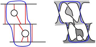
In Figure 8, the EPD exhibits more complicated behavior than in the other examples, in that it bounds nontrivial portions of the graph $H_{A}$. We call an EPD that bounds nontrivial portions of $H_{A}$ on both sides a complex EPD. The minimal number of complex EPDs in the spanning set of the maximal $I$–bundle of $M_{A}$ is denoted $||E_{c}||$, and is exactly the correction term in Theorem 3.5. By analyzing EPDs, we show the following.

One family of knots and links that satisfies Proposition 3.9 is that of alternating links [29]. If $D=D(K)$ is a prime, twist–reduced alternating link diagram, then it is both $A$– and $B$–adequate, and for each 2–edge loop in ${\mathbb{G}_{A}}$ or ${\mathbb{G}_{B}}$, both edges belong to the same twist region. Theorem 3.6 gives lower bounds on volume in terms of both ${\chi_{-}}({\mathbb{G}^{\prime}_{A}})$ and ${\chi_{-}}({\mathbb{G}^{\prime}_{B}})$. By averaging these two lower bounds, one recovers Lackenby’s lower bound on the volume of hyperbolic alternating links, in terms of the twist number $t(D)$.

Theorem 3.6 greatly expands the list of manifolds for which we can compute explicitly the Euler characteristic of the guts, and can be used to derive results analogous to Theorem 3.10. As a sample, we state the following.

Observe that the multiplicative constants in the upper and lower bounds differ by a rather small factor of about $4.155$.

We obtain similarly tight two–sided volume bounds for Montesinos links, using these guts techniques [19].

Similar results using different techniques have been obtained by the authors in [14, 15, 16], and by Purcell in [39].

The main results of [19] explore the idea that the stable coefficient $\beta_{K}^{\prime}$ does an excellent job of measuring the geometric and topological complexity of the manifold $M_{A}=S^{3}{\backslash\backslash}S_{A}$. (Similarly, $\beta_{K}$ measures the complexity of $M_{B}=S^{3}{\backslash\backslash}M_{B}$.)

For instance, note that we have ${\left|\beta^{\prime}_{K}\right|}=1-\chi({\mathbb{G}^{\prime}_{A}})=0$ exactly when $\chi({\mathbb{G}^{\prime}_{A}})=1$, or equivalently ${\mathbb{G}^{\prime}_{A}}$ is a tree. Thus it follows from Theorem 3.2 that $\beta^{\prime}_{K}$ is exactly the obstruction to $S_{A}$ being a fiber.

Similarly, ${\left|\beta_{K}^{\prime}\right|}=1$ precisely when $S_{A}$ is a fibroid of a particular type [19, Theorem 9.18]. In general, the JSJ decomposition of $M_{A}$ contains guts: the non-trivial hyperbolic pieces. In this case, ${\left|\beta_{K}^{\prime}\right|}$ measures the complexity of the guts together with certain complicated parts of the maximal $I$–bundle of $M_{A}$.

The volume conjecture of Kashaev and Murakami–Murakami [28, 36] states that all hyperbolic knots satisfy

If the volume conjecture is true, then for large $n$, there would be a relation between the coefficients of $J^{n}_{K}(t)$ and the volume of the knot complement. In recent years, articles by Dasbach and Lin and the authors have established relations for several classes of knots [11, 14, 15, 16]. However, in all these results, the lower bound involved first showing that the Jones coefficients give a lower bound on twist number, then showing twist number gives a lower bound on volume. Each of these steps is known to fail outside special families of knots [16, 17]. Moreover, the two-step argument is indirect, and the constants produced are not sharp. By contrast, in [19], we bound volume below in terms of ${\chi_{-}}({\rm guts})$, which is directly related to colored Jones coefficients. This yields sharper lower bounds on volumes, along with a more intrinsic explanation for why these lower bounds exist. For instance, Theorems 3.11 and 3.12 have the following corollaries.

To begin, we need to visualize the state surface $S_{A}$ more carefully. We constructed $S_{A}$ by first, taking a collection of disks bounded by state circles, and then attaching bands at crossings. Recall we ensured the disks were below the projection plane. We visualize the disks as soup cans. That is, for each, a long cylinder runs deep under the projection plane with a disk at the bottom. Soup cans will be nested, with outer state circles bounding deeper, wider soup cans. Isotope the diagram so that it lies on the projection plane, except at crossings which run through a crossing ball. When we are finished, the surface $S_{A}$ lies below the projection plane, except for bands that run through a small crossing ball.

In Figure 12, the state surface for this example is shown lying below the projection plane (although soup cans have been smoothed off at their sharp edges in this figure).

We cut $M_{A}=S^{3}{\backslash\backslash}S_{A}$ along disks. These disks come from complementary regions of the graph of the link diagram on the projection plane. Notice that each such region corresponds to a complementary region of the graph $H_{A}$, the graph of the $A$–resolution. To form the disk that we cut along, we isotope the disk by pushing it under the projection plane slightly, keeping its boundary on the state surface $S_{A}$, so that it meets the link a minimal number of times. Indeed, because $S_{A}$ itself lies on or below the projection plane except in the crossing balls, we can push the disk below the projection plane everywhere except possibly along half–twisted rectangles at the crossings. By further isotopy we can arrange each disk so that its boundary runs meets the link only inside the crossing ball. These isotoped disks are called white disks.

For each region of the complement of $H_{A}$, we have a white disk that meets the link only in crossing balls, and then only at under–crossings. The disk lies slightly below the projection plane everywhere. Figure 13 gives an example.

Some of the white disks will not meet the link at all. These disks are isotopic to soup cans on $S_{A}$; that is, they are innermost disks. We will remove all such white disks from consideration. When we do so, the collection of all remaining white disks, denoted ${\mathcal{W}}$, consists of those with boundary on the state surface $S_{A}$ and on the link $K$.

It is actually straightforward to see that the components of $M_{A}{\backslash\backslash}{\mathcal{W}}$ are 3–balls, as follows. There will be a single component above the projection plane. Since we cut along each region of the projection graph, either along a disk of ${\mathcal{W}}$ or an innermost soup can, this component above the projection plane must be homeomorphic to a ball. As for components which lie below the projection plane, these lie between soup can disks. Since any such disk cuts the 3–ball below the projection plane into 3–balls, these components must also each be homeomorphic to 3–balls. In fact, we know more:

The edges of the ideal polyhedron are given by the intersection of white disks in ${\mathcal{W}}$ with (the boundary of a regular neighborhood of) $S_{A}$. Each edge runs between strands of the link. The ideal vertices lie on the torus boundary of the tubular neighborhood of a link component. The regions (faces) come from white disks (white faces) and portions of the surface $S_{A}$, which we shade.

Note that each edge bounds a white disk in ${\mathcal{W}}$ on one side, and a portion of the shaded surface $S_{A}$ on the other side. Thus, by construction, we have a checkerboard coloring of the 2–dimensional regions of our decomposition. Since the white regions are known to be disks, showing that our 3–balls are actually polyhedra amounts to showing that the shaded regions are also simply connected. Showing this requires some work, and the hypothesis of $A$–adequacy is heavily used. The interested reader is referred to [19, Chapter 3] for the details.

We need a simpler description of our polyhedra than that afforded by the 3–dimensional pictures of the last subsection. We obtain 2–dimensional descriptions in terms of how the white and shaded faces are super-imposed on the projection plane, and how these faces interact with the planar graph $H_{A}$. These descriptions are the starting point for our proofs in [19]. In this subsection we briefly highlight the main characteristics of these descriptions.

Note that in the figures, we often use different colors to indicate different shaded faces. All these colored regions come from the surface $S_{A}$.

In the last subsection, we saw that the lower polyhedra correspond to alternating link diagrams. It may happen that one of these alternating diagrams is not prime. In other words, the alternating link diagram contains a pair of regions that meet along more than one edge. The polyhedral analogue of this notion is the following.

Primeness is an extremely desirable property in a polyhedral decomposition, for the following reason. The theory of normal surfaces, developed by Haken [22], states that given a polyhedral decomposition of a manifold $M$, every essential surface $S\subset M$ can be moved into a form where it intersects each polyhedron in standard disks, called normal disks. If this essential surface is (say) a compression disk $D\subset M_{A}$, then we may intersect $D$ with the union of white faces ${\mathcal{W}}$ to form a collection of arcs in $D$. An outermost arc must cut off a bigon. But, by Definition 5.2, a prime polyhedron cannot contain a bigon. Thus, once we obtain a decomposition of $M_{A}$ into prime polyhedra, Theorem 2.4 will immediately follow.

In practice, the polyhedra described in the last subsection may sometimes fail to be prime. Whenever this occurs, we need to cut them into smaller, prime pieces. Before we describe this cutting process, we record another powerful feature of the polyhedral decomposition.

Notice that the polyhedron in Figure 20 is combinatorially a prism over an ideal heptagon: here, the two shaded faces are the horizontal faces of the prism, while the seven white faces are lateral, vertical essential product disks. In other words, the entire polyhedron is an $I$–bundle over an ideal polygon. It turns out that under the hypothesis of primeness, when the upper polyhedron has this product structure, then so do all of the lower polyhedra, and so does the manifold $M_{A}=S^{3}{\backslash\backslash}S_{A}$.

The proof of equivalence of the conditions in Proposition 5.3 is not hard. For example, if every white face is a bigon, then in every polyhedron, those bigons must be strung end to end, forming a cycle of lateral faces in a prism. Note as well that if every polyhedron is a prism, i.e. a product, then this product structure extends over the bigon faces to imply that $M_{A}\cong S_{A}\times I$. This immediately gives one implication in Theorem 3.2: if ${\mathbb{G}^{\prime}_{A}}$ is a tree, then $S_{A}$ is a fiber.

The converse implication (if $S_{A}$ is a fiber, then ${\mathbb{G}^{\prime}_{A}}$ is a tree) requires knowing that our polyhedra detect the JSJ decomposition of $M_{A}$. In other words: if part (or all) of $M_{A}$ is an $I$–bundle, then this $I$–bundle structure must be visible in the individual polyhedra. This property also follows from primeness.

We have seen that primeness is a desirable property of the polyhedral decomposition. Here, we describe a way to detect when a lower polyhedron is not prime, and a way to fix this situation.

Each non-prime arc is lies in a single white face of ${\mathcal{W}}$, while its shadow on the soup can below lies in a single shaded face. Thus every non-prime arc indicates that a lower polyhedron violates Definition 5.2. See Figure 21.

Whenever we find a non-prime arc, we modify the polyhedral decomposition as follows: push the arc $\alpha$ down against the soup can of the state circle $C$. This divides the corresponding lower polyhedron into two. Figure 21 shows a 3–dimensional view of this cutting process.

Combinatorially, we cut a lower polyhedron along the non-prime arc, as in Figure 22. The lower polyhedra now correspond to alternating links whose state circles contain $\alpha$. On the boundary of the upper polyhedron, $\alpha$ meets two tentacles. These will be joined into the same shaded face, by attaching both tentacles to a regular neighborhood of $\alpha$. See Figure 23.

Repeat this process of splitting along non-prime arcs until there are no more non-prime arcs. This ensures that all the lower polyhedra are prime. Then, one can show that the upper polyhedron is prime as well.

A decomposition along a maximal collection of non-prime arcs ${\mathbb{A}}$ is called a prime decomposition. Its main features are summarized as follows:

• •

  It decomposes $M_{A}$ into one upper and at least one lower polyhedron.

• •

  Every polyhedron is prime.

• •

  Every polyhedron is checkerboard colored, with 4–valent vertices.

• •

  White faces of the polyhedra correspond to regions of the complement of $H_{A}\cup{\mathbb{A}}$.

• •

  Lower polyhedra are in one-to-one correspondence with nontrivial complementary regions of $s_{A}\cup{\mathbb{A}}$.

• •

  Each lower polyhedron is identical to the checkerboard polyhedron of an alternating link, where the alternating link is obtained by taking the restriction of $H_{A}\cup{\mathbb{A}}$ to the corresponding region of $s_{A}\cup{\mathbb{A}}$, and replacing segments of $H_{A}$ with crossings (using the $A$–resolution).

References

- [1] Colin C. Adams, Noncompact Fuchsian and quasi-Fuchsian surfaces in hyperbolic 3–manifolds, Alebr. Geom. Topol. 7 (2007), 565–582.
- [2] Ian Agol, Peter A. Storm, and William P. Thurston, Lower bounds on volumes of hyperbolic Haken 3-manifolds, J. Amer. Math. Soc. 20 (2007), no. 4, 1053–1077, with an appendix by Nathan Dunfield.
- [3] Cody Armond and Oliver T. Dasbach, Rogers–Ramanujan type identities and the head and tail of the colored Jones polynomial, arXiv:1106.3948.
- [4] Béla Bollobás and Oliver Riordan, A polynomial invariant of graphs on orientable surfaces, Proc. London Math. Soc. (3) 83 (2001), no. 3, 513–531.
- [5] by same author, A polynomial of graphs on surfaces, Math. Ann. 323 (2002), no. 1, 81–96.
- [6] Abhijit Champanerkar, Ilya Kofman, and Eric Patterson, The next simplest hyperbolic knots, J. Knot Theory Ramifications 13 (2004), no. 7, 965–987.
- [7] Marc Culler and Peter B. Shalen, Volumes of hyperbolic Haken manifolds. I, Invent. Math. 118 (1994), no. 2, 285–329.
- [8] Oliver T. Dasbach, David Futer, Efstratia Kalfagianni, Xiao-Song Lin, and Neal W. Stoltzfus, The Jones polynomial and graphs on surfaces, Journal of Combinatorial Theory Ser. B 98 (2008), no. 2, 384–399.
- [9] by same author, Alternating sum formulae for the determinant and other link invariants, J. Knot Theory Ramifications 19 (2010), no. 6, 765–782.
- [10] Oliver T. Dasbach and Xiao-Song Lin, On the head and the tail of the colored Jones polynomial, Compositio Math. 142 (2006), no. 5, 1332–1342.
- [11] by same author, A volume-ish theorem for the Jones polynomial of alternating knots, Pacific J. Math. 231 (2007), no. 2, 279–291.
- [12] Tudor Dimofte and Sergei Gukov, Quantum field theory and the volume conjecture, Contemp. Math. 541 (2011), 41–68.
- [13] Nathan M. Dunfield and Stavros Garoufalidis, Incompressibility criteria for spun-normal surfaces, Trans. Amer. Math. Soc. 364 (2012), no. 11, 6109–6137.
- [14] David Futer, Efstratia Kalfagianni, and Jessica S. Purcell, Dehn filling, volume, and the Jones polynomial, J. Differential Geom. 78 (2008), no. 3, 429–464.
- [15] by same author, Symmetric links and Conway sums: volume and Jones polynomial, Math. Res. Lett. 16 (2009), no. 2, 233–253.
- [16] by same author, Cusp areas of Farey manifolds and applications to knot theory, Int. Math. Res. Not. IMRN 2010 (2010), no. 23, 4434–4497.
- [17] by same author, On diagrammatic bounds of knot volumes and spectral invariants, Geom. Dedicata 147 (2010), 115–130.
- [18] by same author, Slopes and colored Jones polynomials of adequate knots, Proc. Amer. Math. Soc. 139 (2011), 1889–1896.
- [19] by same author, Guts of surfaces and the colored Jones polynomial, Research monograph to appear in Lecture Notes in Mathematics (Springer), vol. 2069, arXiv:1108.3370.
- [20] Stavros Garoufalidis, The Jones slopes of a knot, Quantum Topol. 2 (2011), no. 1, 43–69.
- [21] Stavros Garoufalidis and Thang T. Q. Lê, The colored Jones function is -holonomic, Geom. Topol. 9 (2005), 1253–1293 (electronic).
- [22] Wolfgang Haken, Theorie der Normalflächen, Acta Math. 105 (1961), 245–375.
- [23] Allen E. Hatcher, On the boundary curves of incompressible surfaces, Pacific J. Math. 99 (1982), no. 2, 373–377.
- [24] Jim Hoste and Morwen B. Thistlethwaite, Knotscape, http://www.math.utk.edu/˜morwen.
- [25] William H. Jaco and Peter B. Shalen, Seifert fibered spaces in -manifolds, Mem. Amer. Math. Soc. 21 (1979), no. 220, viii+192.
- [26] Klaus Johannson, Homotopy equivalences of –manifolds with boundaries, Lecture Notes in Mathematics, vol. 761, Springer, Berlin, 1979.
- [27] Vaughan F. R. Jones, Hecke algebra representations of braid groups and link polynomials, Ann. of Math. (2) 126 (1987), no. 2, 335–388.
- [28] Rinat M. Kashaev, The hyperbolic volume of knots from the quantum dilogarithm, Lett. Math. Phys. 39 (1997), no. 3, 269–275.
- [29] Marc Lackenby, The volume of hyperbolic alternating link complements, Proc. London Math. Soc. (3) 88 (2004), no. 1, 204–224, With an appendix by Ian Agol and Dylan Thurston.
- [30] W. B. Raymond Lickorish, An introduction to knot theory, Graduate Texts in Mathematics, vol. 175, Springer-Verlag, New York, 1997.
- [31] W. B. Raymond Lickorish and Morwen B. Thistlethwaite, Some links with nontrivial polynomials and their crossing-numbers, Comment. Math. Helv. 63 (1988), no. 4, 527–539.
- [32] William W. Menasco, Polyhedra representation of link complements, Low-dimensional topology (San Francisco, Calif., 1981), Contemp. Math., vol. 20, Amer. Math. Soc., Providence, RI, 1983, pp. 305–325.
- [33] by same author, Closed incompressible surfaces in alternating knot and link complements, Topology 23 (1984), no. 1, 37–44.
- [34] Yosuke Miyamoto, Volumes of hyperbolic manifolds with geodesic boundary, Topology 33 (1994), no. 4, 613–629.
- [35] Hitoshi Murakami, An introduction to the volume conjecture, Contemp. Math. 541 (2011), 1–40.
- [36] Hitoshi Murakami and Jun Murakami, The colored Jones polynomials and the simplicial volume of a knot, Acta Math. 186 (2001), no. 1, 85–104.
- [37] Makoto Ozawa, Essential state surfaces for knots and links, J. Aust. Math. Soc. 91 (2011), no. 3, 391–404.
- [38] Józef H. Przytycki, From Goeritz matrices to quasi-alternating links, The mathematics of knots, Contrib. Math. Comput. Sci., vol. 1, Springer, Heidelberg, 2011, pp. 257–316.
- [39] Jessica S. Purcell, Volumes of highly twisted knots and links, Algebr. Geom. Topol. 7 (2007), 93–108.
- [40] Alexander Stoimenow, On the crossing number of semi-adequate links, Preprint available at http://stoimenov.net/stoimeno/homepage/papers/adeq2.pdf.
- [41] Morwen B. Thistlethwaite, On the Kauffman polynomial of an adequate link, Invent. Math. 93 (1988), no. 2, 285–296.
- [42] William P. Thurston, Three-dimensional manifolds, Kleinian groups and hyperbolic geometry, Bull. Amer. Math. Soc. (N.S.) 6 (1982), no. 3, 357–381.
- [43] by same author, A norm for the homology of –manifolds, Mem. Amer. Math. Soc. 59 (1986), no. 339, i–vi and 99–130.
- [44] Vladimir G. Turaev, A simple proof of the Murasugi and Kauffman theorems on alternating links, Enseign. Math. (2) 33 (1987), no. 3-4, 203–225.
- [45] by same author, The Yang-Baxter equation and invariants of links, Invent. Math. 92 (1988), no. 3, 527–553.
- [46] Edward Witten, -dimensional gravity as an exactly soluble system, Nuclear Phys. B 311 (1988/89), no. 1, 46–78.
- [47] by same author, Quantum field theory and the Jones polynomial, Comm. Math. Phys. 121 (1989), no. 3, 351–399.