跳到论文正文
W Papers独立论文阅读器 arXiv:1110.6196 论文正文 计算阅读时间 · 0%
引用这篇论文根据当前论文元数据生成,正式投稿前建议核对。


License: arXiv.org perpetual non-exclusive license
arXiv:1110.6196v1 [cond-mat.mes-hall] 27 Oct 2011

The two dimensional local density of states of a Topological Insulator with an edge dislocation

D. Schmeltzer Affiliation: Physics Department, City College of the City University of New York
New York, New York 10031
Abstract

We investigate the effect of a crystal edge dislocation on the metallic surface of a Topological Insulator. The edge dislocation gives rise to torsion which the electrons experience as a spin connection. As a result the electrons propagate along confined two dimensional regions and circular contours. Due to the edge dislocations the parity symmetry is violated resulting in a current measured by the in-plane component of the spin on the surface. The tunneling density of states for Burger vectors in the yy direction is maximal along the xx direction . The evidence of the enhanced tunneling density of states can be verified with the help of the scanning tunneling technique.

I Introduction

Seldom a new state of matter is predicted. Even less often is it unambiguously observed in the laboratory in the spectacular way was done with HgTe quantum wells [1]. Indeed, this novel two-dimensional (2D) topological insulator (TI) shows a quantized charge conductance, similar to that observed in Quantum Hall effect, without the need to apply a magnetic field. This result triggered further theoretical and experimental work that resulted in the discovery of metallic surface states in the insulating alloy B​ix​S​b1−xBi_{x}Sb_{1-x}, the first three-dimensional topological insulator. In this case, the conducting surface states are formed by topological effects that render the electrons traveling on such surfaces insensitive to scattering by impurities. The theoretical foundations of this phenomena are based on the topology of the Brillouin zone [2, 3, 4, 5, 6, 7, 8, 9, 12, 13, 15, 17, 31, 22]. The theoretical predictions have been confirmed experimentally for the three dimensional (3​D3D) Topological Insulators (T​ITI) B​i2​S​e3Bi_{2}Se_{3}, B​i2​T​e3Bi_{2}Te_{3} and B​i1−x​S​bxBi_{1-x}Sb_{x}. The electronic band structure of these crystals is time reversal invariant obeying Kramer’s theorem T2=−1T^{2}=-1 and have a single Dirac cone which lies in a gap [2, 18, 23, 1]. At the boundary of the 3​D3D T​ITI, one obtains a 2​D2D surface with an odd number of chiral edge excitations coined h​e​l​i​c​a​lhelical l​i​q​u​i​dliquid [37] and realized experimentally in the two-dimensional C​d​T​e/H​g​T​e/C​d​T​eCdTe/HgTe/CdTe quantum wells [1, 36]. The dissipationless surface states are believed to be quantum-protected by the bulk insulator. A variety of transport experiments suggest that the conductivity of a 3​D3D T​ITI contains a significant metallic contribution [39]. Scanning tunneling microscopy (S​T​MSTM) and transmission electron spectroscopy (T​E​MTEM ) of the chiral metallic boundary show that crystal defects modify the density of states. The momentum-resolved Landau spectroscopy of the Dirac surface state in B​i2​S​e3Bi_{2}Se_{3} [38] reveals, in addition to the Landau spectroscopy, triangular-shaped structure caused by the presence of vacancies of B​iBi at the S​eSe sites. These experiments suggest that the two dimensional surface of the T​ITI is sensitive to defects and geometry and therefore, the quantization rules are expected to be modified, and probably are revealed through the new Berry indices γ≠12\gamma\neq\frac{1}{2} [42]. (In a recent Shubnikov-de Haas oscillation experiment performed on the T​ITI B​i2​S​e3Bi_{2}Se_{3} [42] the authors show magnetic oscillations which correspond to the Landau level quantization En=vF​2​(n+γ)​ℏ​e​BE_{n}=v_{F}\sqrt{2(n+\gamma)\hbar eB} with the Berry phase index which is different from γ=12\gamma=\frac{1}{2}.) The appearance of the new indices γ≠12\gamma\neq\frac{1}{2} might be due to topology of the defects or/and interactions. Recently [43] the effect of the δ(2)​(r→)\delta^{(2)}(\vec{r}) impurity potential on the metallic surface of the T​ITI has been shown to modify the local density of states. The authors in ref. [19] have proposed that crystal dislocations generate protected zero modes which give rise to perfect metallic conduction. This idea has been used to explain the thermoelectric transport in the 3​D3D T​ITI [25].

From the theory of quantum crystal [47] three primary types of topological defects are known : e​d​g​eedge d​i​s​l​o​c​a​t​i​o​n​sdislocations, s​c​r​e​wscrew d​i​s​l​o​c​a​t​i​o​n​sdislocations and m​i​x​e​dmixed d​i​s​l​o​c​a​t​i​o​n​sdislocations. The strength of the dislocations is measured in units of of the B​u​r​g​e​rBurger vectors which corresponds to the shortest lattice translation in the crystal. Experimentally, the dislocations are seen as dark lines in the lighter central regions of the transmission electron micrograph.

The dislocations induce crystal stresses which are characterized by the Burger vector, shear modulus and Poisson’s ratio [47, 33]. As a result, the lattice vibrations are complicated and the electron-phonon interaction plays a crucial role in inducing new dynamical effects. We will ignore the dynamical effects and concentrate on the static effects caused by the elastic strain field on the electrons. In a crystal we have the neutrality condition, namely the sum of the Burger vectors must be zero. We consider first a single dislocation (one assumes that a second dislocation with an opposite Burger vector is located far away from the first dislocation) and in the second stage we generalize the results to an even number of dislocations.

Thirty two years ago the propagation of electrons in the presence of a dislocated crystal was investigated [26]. Those calculations, performed with the Schrödinger equation, revealed the possibility for interesting electronic transport. For a screw dislocation, the Schrödinger equation is equivalent to the Aharonov-Bohm problem in two dimensions [27] which hints that the physics of persistent currents might play a crucial role . In graphene, different topological defects such as crystal d​i​s​c​l​i​n​a​t​i​o​n​sdisclinations have been modeled as a vortex field [29, 28].

We start our discussion with the Peierls model [20] which is an approximation for the edge dislocations without torsion . This model gives results which are in agreement with those obtained by [19] for the 3​D3D T​ITI. For this model we find that at the boundary of the dislocation a zero mode exist and confines the electrons to the dislocation line.

Unfortunately, the Peierls model represents a over- simplification of the reality. The model is lacking torsion which is an important property for dislocations. A complete description of the edge dislocation must include the t​o​r​s​i​o​ntorsion tensor . This tensor generates spin connections [44, 45, 46, 22] which are controlled by the B​u​r​g​e​rBurger vector. Using the complete description of the edge dislocation we find that the electronic excitations are confined to a two dimensional region and to a set of circular contours. Such structure can be studied using the formulation introduced in ref. [51, 50, 52]. The circular contours have a radius Rg​(n)R_{g}(n) n=±1,±2,±3,…n=\pm 1,\pm 2,\pm 3,... which are determined by the strength of the Burger vector. Comparing the results obtained from the model with torsion to the one obtained from the Peierls model, we find that the torsion destroys the zero mode state, but due to the Parity violation the system is only weakly affected by backscattering.

The contents of this paper is as follows: In chapter II we present the chiral model for the boundary surface of the T​ITI. Chapter III is devoted to the edge dislocation. We devote a short discussion to the Peierls model and present an extended derivation for the effect of dislocations on the T​ITI. Chapter IV is devoted to the solution of the wave function in the presence of an edge dislocation. Chapter V presents the explicit wave functions for the two dimensional region and circular contours. Chapter VI presents the the computation of the tunneling density of states induced by the edge dislocation. In chapter VII we show that the violation of the parity symmetry by the edge dislocation generates a current which has an in-plane spin component. We suggest that this current which confirms the presence of the edge dislocation might be measured using Magnetic Force Microscopy techniques. Chapter VIII is devoted to conclusions.

II-The chiral metal - the boundary surface of the three dimensional Topological Insulator

The low energy Hamiltonian for the bulk 3​D3D T​ITI in the B​i2​S​e3Bi_{2}Se_{3} family was shown to behave on the boundary surface (the x,yx,y- plane) as a two dimensional chiral metal [11] which is similar the Rashba [10] model.

H=∫d2rΨ†(r→)[hT.I(x,y)−μ]Ψ(r→)]≡ℏvF∫d2rΨ†(r→)[iσ1∂y−iσ2∂x−μ]Ψ(r→)\displaystyle H=\int\,d^{2}r\Psi^{\dagger}(\vec{r})[h^{T.I}(x,y)-\mu]\Psi(\vec{r})]\equiv\hbar v_{F}\int\,d^{2}r\Psi^{\dagger}(\vec{r})[i\sigma^{1}\partial_{y}-i\sigma^{2}\partial_{x}-\mu]\Psi(\vec{r})

hT.I(x,y)=ℏvF[iσ1∂y−iσ2∂x]h^{T.I}(x,y)=\hbar v_{F}[i\sigma^{1}\partial_{y}-i\sigma^{2}\partial_{x}] is the chiral Dirac Hamiltonian in the first quantized language. vF≈5⋅105​ms​e​cv_{F}\approx 5\cdot 10^{5}\frac{m}{sec} is the Fermi velocity, σ\sigma is the Pauli matrix describing the electron spin and μ\mu is the chemical potential measured relative to the Dirac Γ\Gamma point. The Hamiltonian for the two dimensional surface L×LL\times L describes well the excitations smaller than the bulk gap of the 3​D3D T​ITI at 0.30.3 e​VeV. Moving away from the Γ\Gamma point, the Fermi velocity becomes momentum dependent; therefore, we will introduce a momentum cut off Λ\Lambda to restrict the validity of the Dirac model. The chiral Dirac model in the Bloch representation takes the form: h=ℏ​vF​(K→×σ→)⋅z^≡ℏ​vF​(−σ1​ky+σ2​kx)h=\hbar v_{F}(\vec{K}\times\vec{\sigma})\cdot\hat{z}\equiv\hbar v_{F}(-\sigma^{1}k_{y}+\sigma^{2}k_{x}) where periodic boundary conditions imply kx=2​πL​mxk_{x}=\frac{2\pi}{L}m_{x} , mx=0,±1,±2,..m_{x}=0,\pm 1,\pm 2,.. and ky=2​πL​myk_{y}=\frac{2\pi}{L}m_{y} , my=0,±1,±2,..m_{y}=0,\pm 1,\pm 2,... The eigen-spinors for this Hamiltonian are : |u(K→)>=[|u↑(K→)>,|u↓(K→)>]T=|K→>⊗[1,iei​χ​(kx,ky)]T|u(\vec{K})>=[|u_{\uparrow}(\vec{K})>,|u_{\downarrow}(\vec{K})>]^{T}=|\vec{K}>\otimes[1,ie^{i\chi(k_{x},k_{y})}]^{T} where χ⁡(kx,ky)=t​a​n−1​(kykx)\chi(k_{x},k_{y})=tan^{-1}(\frac{k_{y}}{k_{x}}) is the spinor phase and ϵ=ℏ​vF​kx2+ky2\epsilon=\hbar v_{F}\sqrt{k^{2}_{x}+k^{2}_{y}} is the eigenvalue for particles . For holes we have the eigenvalue ϵ=−ℏ​vF​kx2+ky2\epsilon=-\hbar v_{F}\sqrt{k^{2}_{x}+k^{2}_{y}} and eigenvectors |v(K→)>=[|v↑(K→)>,|v↓(K→)>]T=|K→>⊗[−1,iei​χ​(kx,ky)]T|v(\vec{K})>=[|v_{\uparrow}(\vec{K})>,|v_{\downarrow}(\vec{K})>]^{T}=|\vec{K}>\otimes[-1,ie^{i\chi(k_{x},k_{y})}]^{T}. The chirality operator is defined in terms of the chiral phase χ⁡(kx,ky)\chi(k_{x},k_{y}):

(σ→×K→|K→|)⋅z^≡sin⁡[χ⁡(kx,ky)]​σ1−cos⁡[χ⁡(kx,ky)]​σ2(\vec{\sigma}\times\frac{\vec{K}}{|\vec{K}|})\cdot\hat{z}\equiv\sin[\chi(k_{x},k_{y})]\sigma^{1}-\cos[\chi(k_{x},k_{y})]\sigma^{2} (2)

The chirality operator takes the eigenvalue −- (counter-clockwise) for particles [sin(χ(kx,ky))σ1−cos(χ(kx,ky))σ2]|K→>⊗[1,iei​χ​(kx,ky)]T=−|K→>⊗[1,iei​χ​(kx,ky)]T[\sin(\chi(k_{x},k_{y}))\sigma^{1}-\cos(\chi(k_{x},k_{y}))\sigma^{2}]|\vec{K}>\otimes[1,ie^{i\chi(k_{x},k_{y})}]^{T}=-|\vec{K}>\otimes[1,ie^{i\chi(k_{x},k_{y})}]^{T} and ++ (clockwise) for holes [sin(χ(kx,ky))σ1−cos(χ(kx,ky))σ2]|K→>⊗[−1,iei​χ​(kx,ky)]T=|K→>⊗[−1,iei​χ​(kx,ky)]T[\sin(\chi(k_{x},k_{y}))\sigma^{1}-\cos(\chi(k_{x},k_{y}))\sigma^{2}]|\vec{K}>\otimes[-1,ie^{i\chi(k_{x},k_{y})}]^{T}=|\vec{K}>\otimes[-1,ie^{i\chi(k_{x},k_{y})}]^{T}. The Hamiltonian hT.I​(K→)=ℏ​vF​(−σ1​ky+σ2​kx)h^{T.I}(\vec{K})=\hbar v_{F}(-\sigma^{1}k_{y}+\sigma^{2}k_{x}) is time reversal invariant hT.I.​(−K→)=T​hT.I.​(K→)​T−1h^{T.I.}(-\vec{K})=Th^{T.I.}(\vec{K})T^{-1} (T=(−i​σy)​K0T=(-i\sigma_{y})K_{0} is the time reversal operator and K0K_{0} is the conjugation operator). At K→=0\vec{K}=0 we have hT.I.​(K→=0)=T​hT.I.​(K→=0)​T−1h^{T.I.}(\vec{K}=0)=Th^{T.I.}(\vec{K}=0)T^{-1} therefore the eigenstate is a Kramer degenerate. The eigenstate |u(K→)>|u(\vec{K})> obeys T2|u(K→)>=−|u(K→)>T^{2}|u(\vec{K})>=-|u(\vec{K})>. The states |u(K→)>|u(\vec{K})> and T|u⁡(K→)>T|u(\vec{K})> are orthogonal to each other. Since T|u⁡(K→)>∝|u⁡(−K→)>T|u(\vec{K})>\propto|u(-\vec{K})> the property T2=−1T^{2}=-1 guarantees that backscattering is prohibited.

III-The edge dislocation on the metallic Surface of the three dimensional Topological Insulator

A-The Peierls model for the edge dislocation

We start our presentation with the Peierls phenomenogical model [20] which might be useful for a large number of dislocations. An edge dislocation in two dimensions can be formulated in the following way: We cut the the two dimensional crystal into two halves (y<0y<0 and y>0y>0). After cutting the crystal along the line y=0y=0, two surfaces [x,y<0][x,y<0] and [x,y>0][x,y>0] have been created. We glue back the two halves by translating by minus one half of the lattice spacing along xx for y<0y<0 and one half along xx for y>0y>0. This procedure creates a dislocation along the line y=0y=0 with a Burger vector along yy , B(2)B^{(2)}. We introduce a distribution of dislocations ρ⁡(x,y)\rho(x,y) then the quantity ρ⁡(x,y)​d​x​d​y\rho(x,y)dxdy represents the Burger vector passing through the area d​x​d​ydxdy. In order to understand the effect of the dislocations on the chiral fermions, we rewrite the two dimensional model on a lattice. On a lattice the model is characterized by the hopping matrix elements t=t0t=t_{0} (for opposite spins) and t′=t0′t^{\prime}=t^{\prime}_{0} ( for parallel spins). In the absence of the Peierls deformation the lattice model takes the form:

HL=∑[x=n​a,y=m​a]Ψ†​(r→)​[σx​(−i​t)​∂^y+σy​(i​t)​∂^x]​Ψ​(r→)+Ψ†​(r→)​[σz​(−2​t′+M)]​Ψ​(r→)\displaystyle H^{L}=\sum_{[x=na,y=ma]}\Psi^{\dagger}(\vec{r})[\sigma^{x}(-it)\hat{\partial}_{y}+\sigma^{y}(it)\hat{\partial}_{x}]\Psi(\vec{r})+\Psi^{\dagger}(\vec{r})[\sigma^{z}(-2t^{\prime}+M)]\Psi(\vec{r})
+(−2​t′)​Ψ†​(r→)​∇^x​Ψ​(r→)+(−2​t′)​Ψ†​(r→)​∇^y​Ψ​(r→)\displaystyle+(-2t^{\prime})\Psi^{\dagger}(\vec{r})\hat{\nabla}_{x}\Psi(\vec{r})+(-2t^{\prime})\Psi^{\dagger}(\vec{r})\hat{\nabla}_{y}\Psi(\vec{r})

where ∂^y\hat{\partial}_{y}, ∂^x\hat{\partial}_{x} represents the d​i​s​c​r​e​t​ediscrete lattice derivatives and the action of the discrete operators ∇^x\hat{\nabla}_{x} ∇^y\hat{\nabla}_{y} on the field operator is: ∇^x​Ψ​(r→)≡Ψ⁡(r→+ax)+Ψ⁡(r→−ax)−2​Ψ​(r→)\hat{\nabla}_{x}\Psi(\vec{r})\equiv\Psi(\vec{r}+a_{x})+\Psi(\vec{r}-a_{x})-2\Psi(\vec{r}) and ∇^y​Ψ​(r→)≡Ψ⁡(r→+ay)+Ψ⁡(r→−ay)−2​Ψ​(r→)\hat{\nabla}_{y}\Psi(\vec{r})\equiv\Psi(\vec{r}+a_{y})+\Psi(\vec{r}-a_{y})-2\Psi(\vec{r}). When 2​t0′=M2t^{\prime}_{0}=M we obtain the chiral model given in eq.(1)(1).

HL≈∑[x=n​a,y=m​a]Ψ†​(r→)​[σx​(−i​t)​∂^y+σy​(i​t)​∂^x]​Ψ​(r→)H^{L}\approx\sum_{[x=na,y=ma]}\Psi^{\dagger}(\vec{r})[\sigma^{x}(-it)\hat{\partial}_{y}+\sigma^{y}(it)\hat{\partial}_{x}]\Psi(\vec{r}) (4)

Following [20] we use the explicit form of the deformation field introduced by the dislocations OPENu⁡(y)=B(2)π​tan−1⁡(yW~))u(y)=\frac{B^{(2)}}{\pi}\tan^{-1}(\frac{y}{\widetilde{W}})). According to the elasticity theory, the Peierls edge dislocation [47] is determined by the half width W~\widetilde{W} function and Burger vector B(2)B^{(2)}: ρ⁡(y)​d​y=B(2)\rho(y)dy=B^{(2)}, ρ⁡(y)=−d​ud​y\rho(y)=-\frac{du}{dy},    u⁡(y)∝M⁡(y)=B(2)π​tan−1⁡(yW~)u(y)\propto M(y)=\frac{B^{(2)}}{\pi}\tan^{-1}(\frac{y}{\widetilde{W}}). Replacing the coordinates [x,y][x,y] by the deformed one, [X⁡(r→),Y⁡(r→)][X(\vec{r}),Y(\vec{r})] we introduce the deformed matrix elements t′≠t′0t^{{}^{\prime}}\neq t^{{}^{\prime}}_{0} : t′=t0′+(∂t′0∂u⁡(y))u(y)t^{{}^{\prime}}=t^{{}^{\prime}}_{0}+(\frac{\partial t^{{}^{\prime}}_{0}}{\partial_{u(y)}})u(y). As a result we find: −2​t′+M=(−2​t0′+M)−2​(∂t′0∂u⁡(y))​u​(y)≡0−ℏ​vF​κ​u​(y)-2t^{\prime}+M=(-2t^{\prime}_{0}+M)-2(\frac{\partial t^{{}^{\prime}}_{0}}{\partial_{u(y)}})u(y)\equiv 0-\hbar v_{F}\kappa u(y) where ℏ​vF≡2​t0\hbar v_{F}\equiv 2t_{0} , κ=1t0​(∂t′0∂u⁡(y))\kappa=\frac{1}{t_{0}}(\frac{\partial t^{{}^{\prime}}_{0}}{\partial_{u(y)}}). As a result we obtain the Peierls Hamiltonian which is similar to the domain wall model introduced by [32].

ϵ​ψ​(x,y)=hP​e​i​e​r​l​s​(x,y)​ψ​(x,y)\displaystyle\epsilon\psi(x,y)=h^{Peierls}(x,y)\psi(x,y)
hP​e​i​e​r​l​s(x,y)=ℏvF[−iσx∂y+iσy∂x−σzκM(y)]\displaystyle h^{Peierls}(x,y)=\hbar v_{F}[-i\sigma^{x}\partial_{y}+i\sigma^{y}\partial_{x}-\sigma^{z}\kappa M(y)]
σy​ψλ​(x,y)=λ​ψλ​(x,y);λ=±1;\displaystyle\sigma^{y}\psi_{\lambda}(x,y)=\lambda\psi_{\lambda}(x,y);\hskip 7.22743pt\lambda=\pm 1;\hskip 14.45377pt

The eigenfunction for the Peierls model obeys periodic boundary conditions in the xx direction ψ⁡(x+L,y)=ψ⁡(x,y)\psi(x+L,y)=\psi(x,y). Therefore the eigen- spinor is given by : ψ(x,y)=ei​p​xΦ(y),p=2​πLm,m=0,±1,±2,…\psi(x,y)=e^{ipx}\Phi(y),\hskip 14.45377ptp=\frac{2\pi}{L}m,\hskip 14.45377ptm=0,\pm 1,\pm 2,.... The eigenvalue ϵ\epsilon is replaced by EE where E≡ϵ−ℏ​vF​pE\equiv\epsilon-\hbar v_{F}p. We observe that if ψ⁡(x,y)\psi(x,y) is an eigenfunction with the eigenvalue EE, the eigenfunction σy​ψ​(x,y)\sigma^{y}\psi(x,y) corresponds to the eigenvalue −E-E. E=0E=0 corresponds to the eigenvalue ϵ=ℏ​vF​p\epsilon=\hbar v_{F}p with the zero mode wave function ψ0​(x,y,p)\psi_{0}(x,y;p) given by :

ψ0(x,y;p)=ei​p​x(θ[y]e−κ​B(2)π∫0ydy′tan−1(y′W~)(1i)+θ[−y]eκ​B(2)π​∫0yd​y′​tan−1⁡(y′W~)(1−i))Φ(0)\displaystyle\psi_{0}(x,y;p)=e^{ipx}(\theta[y]e^{-\frac{\kappa B^{(2)}}{\pi}\int_{0}^{y}\,dy^{\prime}\tan^{-1}(\frac{y^{\prime}}{\widetilde{W}})}\left(\begin{array}[]{cc}1\\ i\end{array}\right)+\theta[-y]e^{\frac{\kappa B^{(2)}}{\pi}\int_{0}^{y}\,dy^{\prime}\tan^{-1}(\frac{y^{\prime}}{\widetilde{W}})}\left(\begin{array}[]{cc}1\\ -i\end{array}\right))\Phi(0)

θ⁡[y]\theta[y] represents the step function which is one for y>0y>0 and zero otherwise. As a result, we obtain for B(2)>0B^{(2)}>0 only a single zero mode with λ=1\lambda=1 for y<0y<0 and λ=−1\lambda=-1 for y>0y>0. The eigenstate given in eq.(6)(6), |U0(p)>|U_{0}(p)> and |U0(−p)>|U_{0}(-p)> are related by the time reversal symmetry T|U0​(p)>∝|U0​(−p)>T|U_{0}(p)>\propto|U_{0}(-p)>. From the equations T2=−1T^{2}=-1 and T|U0​(p)>∝|U0​(−p)>T|U_{0}(p)>\propto|U_{0}(-p)> we conclude that the zero mode state is stable against backscattering along the xx direction. ( The states |U0(p)>|U_{0}(p)> and |U0(−p)>|U_{0}(-p)> are defined according to their wave functions <x,y|U0​(p)>≡ψ0​(x,y,p)<x,y|U_{0}(p)>\equiv\psi_{0}(x,y;p) , <x,y|U0​(−p)>≡ψ0​(x,y,−p)<x,y|U_{0}(-p)>\equiv\psi_{0}(x,y;-p).)

B-The edge dislocation with with a non zero torsion Tμ,ν(2)T^{(2)}_{\mu,\nu}

For the remaining part, we will limit our discussion to the microscopic formulation of dislocations. When an edge dislocation is introduced into the crystal, the lattice coordinates r→=(x,y)\vec{r}=(x,y) are modified, r→→R→=r→+u→≡[X⁡(r→),Y⁡(r→)]\vec{r}\rightarrow\vec{R}=\vec{r}+\vec{u}\equiv[X(\vec{r}),Y(\vec{r})] where u→​(r→)\vec{u}(\vec{r}) is the local lattice deformation with the core at the dislocation centered at r→=(0,0)\vec{r}=(0,0). The elastic field contour integral around the core r→=(0,0)\vec{r}=(0,0) is determined by the Burger vector B(a)B^{(a)}, a=1,2a=1,2: ∮d​xμ​∂μu(a)​(r→)=−B(a)\displaystyle\oint dx^{\mu}\partial_{\mu}u^{(a)}(\vec{r})=-B^{(a)}. For an edge dislocation in the xx direction the B​u​r​g​e​rBurger vector B(2)B^{(2)} is in the yy direction . The value of the burger vector B(2)B^{(2)} is given by the shortest translation lattice vector in the yy direction. (For the T​ITI B​i2​S​e3Bi_{2}Se_{3} the length of the vector B(2)B^{(2)} is 55 times the inter atomic distance ). For the two dimensional surface we use the notation xμx^{\mu} ,μ=x,y\mu=x,y for the fixed Cartesian coordinate and XaX^{a} ,a=1,2a=1,2 to describe the reference frame , the media with dislocations. In the media with dislocations we introduced a set of vectors eae_{a} which are orthogonal to each other (eb,ea)≡<eb|ea>=δab(e_{b},e_{a})\equiv<e^{b}|e_{a}>=\delta^{b}_{a}. The unit vector eae_{a} can be represented in terms of the Cartesian fixed frame space with the coordinate basis ∂μ\partial_{\mu} ,μ=x,y\mu=x,y. The basis in the media frame can be expanded in terms of the fixed Cartesian frame ∂μ\partial_{\mu}; we have : ea=eμa∂μe_{a}=e^{\mu}_{a}\partial_{\mu} (for the particular case where vectors eae_{a} are given by ea=∂ae_{a}=\partial_{a} the transformation between the two basis is eaμ=δaμe^{\mu}_{a}=\delta^{\mu}_{a}). Any vector X→\vec{X} can be represented in terms of the unit vectors eae_{a} (in the dislocation space) and ∂μ\partial_{\mu} in the Cartesian fixed coordinates space , X→=Xaea=Xμ∂μ\vec{X}=X^{a}e_{a}=X^{\mu}\partial_{\mu}. The dual vector eae^{a} is a o​n​eone f​o​r​mform and can be expanded in terms of the one forms d​xμdx^{\mu}. We have ea=eμa​d​xe^{a}=e^{a}_{\mu}dx, where eμae^{a}_{\mu} represents the matrix transformation ea≡(∂μXa)​d​xμe^{a}\equiv(\partial_{\mu}X^{a})dx^{\mu}. The scalar product of the components eμa​eνa=gμ,νe^{a}_{\mu}e^{a}_{\nu}=g_{\mu,\nu}, eaν​ebν=δa,be^{\nu}_{a}e^{\nu}_{b}=\delta_{a,b} defines the metric tensors, gμ,νg_{\mu,\nu} (in the Cartesian frame ) and δa,b\delta_{a,b} in the dislocation frame. We will compute the matrix elements fields eμae^{a}_{\mu} for our problem :

eμa=∂μXa(r→);a=1,2;μ=x,ye^{a}_{\mu}=\partial_{\mu}X^{a}(\vec{r});\hskip 7.22743pta=1,2;\hskip 7.22743pt\mu=x,y (12)

Following [33] we can express the Burger vector in terms of the the partial derivatives with respect the coordinates a=1,2a=1,2 in the dislocation frame and μ=x,y\mu=x,y for the fixed Cartesian frame :

∂xey2−∂yex2=B(2)​δ2​(r→)\partial_{x}e^{2}_{y}-\partial_{y}e^{2}_{x}=B^{(2)}\delta^{2}(\vec{r}) (13)

Using Stokes theorem, we replace the line integral ∮d​xμ​eμ2​(r→)\displaystyle\oint dx^{\mu}e^{2}_{\mu}(\vec{r}) by the surface integral ∫∫⁡d​xμ​d​xν​[∂xey2−∂yex2]\int\int dx^{\mu}dx^{\nu}[\partial_{x}e^{2}_{y}-\partial_{y}e^{2}_{x}]. For a system with zero c​u​r​v​a​t​u​r​ecurvature and non zero t​o​r​s​i​o​ntorsion Tμ,ν(2)T^{(2)}_{\mu,\nu} we find that the surface torsion tensor integral ∫∫⁡d​xμ​d​xν​Tμ,ν(2)\int\int dx^{\mu}dx^{\nu}T^{(2)}_{\mu,\nu} is equal to ∫∫⁡d​xμ​d​xν​[∂xey2−∂yex2]\int\int dx^{\mu}dx^{\nu}[\partial_{x}e^{2}_{y}-\partial_{y}e^{2}_{x}], and therefore both integrals are equal to the Burger vector.

∮d​xμ​eμ2​(r→)=∫∫⁡d​xμ​d​xν​[∂μeν2−∂νeμ2]=B(2);\displaystyle\displaystyle\oint dx^{\mu}e^{2}_{\mu}(\vec{r})=\int\int dx^{\mu}dx^{\nu}[\partial_{\mu}e^{2}_{\nu}-\partial_{\nu}e^{2}_{\mu}]=B^{(2)};
∫∫⁡d​xμ​d​xν​Tμ,ν(2)=∫∫⁡d​xμ​d​xν​[∂μeν2−∂νeμ2]=B(2);\displaystyle\int\int dx^{\mu}dx^{\nu}T^{(2)}_{\mu,\nu}=\int\int dx^{\mu}dx^{\nu}[\partial_{\mu}e^{2}_{\nu}-\partial_{\nu}e^{2}_{\mu}]=B^{(2)};
∂xey2−∂yex2=B(2)​δ2​(r→)\displaystyle\partial_{x}e^{2}_{y}-\partial_{y}e^{2}_{x}=B^{(2)}\delta^{2}(\vec{r})

where d​xμ​d​xνdx^{\mu}dx^{\nu} represents the surface element. The tangent components eμae^{a}_{\mu} can be expressed in terms of the Burger vector density B(2)​δ2​(r→)B^{(2)}\delta^{2}(\vec{r}) [34] :

ex2=(B(2)2​π)​y(x2+y2);ey2=1−(B(2)2​π)​x(x2+y2)\displaystyle e^{2}_{x}=(\frac{B^{(2)}}{2\pi})\frac{y}{(x^{2}+y^{2})};\hskip 21.68121pte^{2}_{y}=1-(\frac{B^{(2)}}{2\pi})\frac{x}{(x^{2}+y^{2})}
ex1=1;ey1=0\displaystyle e^{1}_{x}=1;\hskip 28.90755pte^{1}_{y}=0 (15)

Using the tangent components, we obtain the metric tensor gμ,νg_{\mu,\nu}.

eμa​eνa≡eμ1​eν1+eμ2​eν2=gμ,ν​(r→);eμa​eμb≡exa​exb+eya​eyb=δa,be^{a}_{\mu}e^{a}_{\nu}\equiv e^{1}_{\mu}e^{1}_{\nu}+e^{2}_{\mu}e^{2}_{\nu}=g_{\mu,\nu}(\vec{r});\hskip 7.22743pte^{a}_{\mu}e^{b}_{\mu}\equiv e^{a}_{x}e^{b}_{x}+e^{a}_{y}e^{b}_{y}=\delta_{a,b} (16)

The inverse of the metric tensor gμ,ν​(r→)g_{\mu,\nu}(\vec{r}) is the tensor gν,μ​(r→)g^{\nu,\mu}(\vec{r}) defined trough the equation gμ,τ​(r→)​gτ,ν​(r→)=δμνg_{\mu,\tau}(\vec{r})g^{\tau,\nu}(\vec{r})=\delta_{\mu}^{\nu}. Using the tangent vectors, we find t​oto f​i​r​s​tfirst o​r​d​e​rorder in the Burger vector the metric tensor gμ,νg_{\mu,\nu} and the Jacobian transformation G\sqrt{G}:

gx,x=1;gx,y=B(2)2​π​yx2+y2;gy,y=1−B(2)2​π​yx2+y2;gy,x=0;G=d​e​t​[gμ,ν]=1−B(2)2​π​yx2+y2g_{x,x}=1;\hskip 7.22743ptg_{x,y}=\frac{B^{(2)}}{2\pi}\frac{y}{x^{2}+y^{2}};\hskip 7.22743ptg_{y,y}=1-\frac{B^{(2)}}{2\pi}\frac{y}{x^{2}+y^{2}};\hskip 7.22743ptg_{y,x}=0;\hskip 7.22743ptG=det[g_{\mu,\nu}]=1-\frac{B^{(2)}}{2\pi}\frac{y}{x^{2}+y^{2}} (17)

The inverse tensor is given by:gx,x≈1g^{x,x}\approx 1, gx,y=gy,x=−B(2)2​π​yx2+y2g^{x,y}=g^{y,x}=-\frac{B^{(2)}}{2\pi}\frac{y}{x^{2}+y^{2}}, gy,y=1+B(2)π​xx2+y2g^{y,y}=1+\frac{B^{(2)}}{\pi}\frac{x}{x^{2}+y^{2}}. Using the inverse tensor gμ,νg^{\mu,\nu} we obtain the inverse matrix eaμe^{\mu}_{a} which is given by:

eaμ=ea,ν​gν,μ=(δa,b​eνb)​gν,μ=eνa​gν,μe^{\mu}_{a}=e_{a,\nu}g^{\nu,\mu}=(\delta_{a,b}e^{b}_{\nu})g^{\nu,\mu}=e^{a}_{\nu}g^{\nu,\mu} (18)

In figure 1 we show the coordinate transformation r→=(x,y)→[X⁡(r→)=x,Y⁡(r→)=y+B(2)2​π​tan−1⁡(yx)]\vec{r}=(x,y)\rightarrow[X(\vec{r})=x,Y(\vec{r})=y+\frac{B^{(2)}}{2\pi}\tan^{-1}(\frac{y}{x})] with the core of the dislocation centered at r→=(0,0)\vec{r}=(0,0).

Next we consider the effect of the dislocation on the T​ITI Hamiltonian. Using the components eaμe^{\mu}_{a} we compute the the transformed Pauli matrices. The Hamiltonian in the absence of the edge dislocation is given by hT.I.=iγa∂a≡∑a=1,2iγa∂ah^{T.I.}=i\gamma^{a}\partial_{a}\equiv\sum_{a=1,2}i\gamma^{a}\partial_{a} where the Pauli matrices are given by γ1=−σ2\gamma^{1}=-\sigma^{2} , γ2=σ1\gamma_{2}=\sigma_{1} and γ3=σ3\gamma^{3}=\sigma^{3}. (We will use the convention that when an index appears twice we perform a summation over this index.) In the presence of the edge dislocation, the term γa∂a\gamma^{a}\partial_{a} must be expressed in terms of the Cartesian fixed coordinates μ=x,y,z\mu=x,y,z. As a result, the spinor Ψ⁡(r→)\Psi(\vec{r}) transforms accordingly to the S​U​(2)SU(2) transformation . If Ψ~​(R→)\widetilde{\Psi}(\vec{R}) is the spinor for the deformed lattice, it can be related with the help of an S​U​(2)SU(2) transformation to the spinor Ψ⁡(r→)\Psi(\vec{r}) in the undeformed lattice: Ψ~​(X,Y)=e−i​δ​φ​(x,y)2​σ3​Ψ​(x,y)\widetilde{\Psi}(X,Y)=e^{-i\frac{\delta\varphi(x,y)}{2}\sigma^{3}}\Psi(x,y) . Where δ​φ​(x,y)\delta\varphi(x,y) is the rotation angle between the two set of coordinates: δ​φ​(x,y)=t​a​n−1​(YX)−t​a​n−1​(yx)\delta\varphi(x,y)=tan^{-1}(\frac{Y}{X})-tan^{-1}(\frac{y}{x}). Using the relation between the coordinates (see figure 1) X=xX=x, and Y=y+B(2)2​π​t​a​n−1​(yx)Y=y+\frac{B^{(2)}}{2\pi}tan^{-1}(\frac{y}{x}) with the singularity at x=y=0x=y=0 gives us that the derivative of the phase which is a delta function, ∂xδφ(x,y)=−∂yδφ(x,y)∝δ2(x,y)\partial_{x}\delta\varphi(x,y)=-\partial_{y}\delta\varphi(x,y)\propto\delta^{2}(x,y). Combining the transformation of the derivative with the S​O​(2)SO(2) rotation in the plane, we obtain the form of the chiral Dirac equation in the Cartesian space (see Appendix A) given in terms of the s​p​i​nspin c​o​n​n​e​c​t​i​o​nconnection ωμ1,2\omega_{\mu}^{1,2} [31]:

iγa∂aΨ~(R→)=iδa,bγb∂aΨ~(R→)=iγaeaμ[∂μ+14[γb,γc]ωμb​c]Ψ(r→)i\gamma_{a}\partial_{a}\widetilde{\Psi}(\vec{R})=i\delta_{a,b}\gamma^{b}\partial_{a}\widetilde{\Psi}(\vec{R})=i\gamma^{a}e^{\mu}_{a}[\partial_{\mu}+\frac{1}{4}[\gamma^{b},\gamma^{c}]\omega_{\mu}^{bc}]\Psi(\vec{r}) (19)

The Hamiltonian hT.I.→he​d​g​eh^{T.I.}\rightarrow h^{edge} is transformed to the dislocation edge Hamiltonian with the explicit form given by:

he​d​g​e=iσ1∂2−iσ2∂1=iσ1e2μ[∂μ+18[σ1,σ1]ωμ1,2]−iσ2e1μ[∂μ+18[σ1,σ1]ωμ1,2]\displaystyle h^{edge}=i\sigma^{1}\partial_{2}-i\sigma^{2}\partial_{1}=i\sigma^{1}e^{\mu}_{2}[\partial_{\mu}+\frac{1}{8}[\sigma^{1},\sigma^{1}]\omega^{1,2}_{\mu}]-i\sigma^{2}e^{\mu}_{1}[\partial_{\mu}+\frac{1}{8}[\sigma^{1},\sigma^{1}]\omega^{1,2}_{\mu}]
=i(σ1e2μ−σ2e1μ)(∂μ+18[σ1,σ2]ωμ1,2)\displaystyle=i(\sigma^{1}e^{\mu}_{2}-\sigma^{2}e^{\mu}_{1})(\partial_{\mu}+\frac{1}{8}[\sigma^{1},\sigma^{2}]\omega^{1,2}_{\mu})

To first order in the Burger vector we find : ωx12=−ωx21=0\omega_{x}^{12}=-\omega_{x}^{21}=0 and −ωy21=ωy1,2=−B(2)2​δ2​(r→)-\omega_{y}^{21}=\omega_{y}^{1,2}=-\frac{B^{(2)}}{2}\delta^{2}(\vec{r}), see eqs. (69−71)(69-71) in Appendix A.

he​d​g​e≈iσ1(∂y−i2σ3B(2)δ2(r→))−iσ2∂xh^{edge}\approx i\sigma^{1}(\partial_{y}-\frac{i}{2}\sigma^{3}B^{(2)}\delta^{2}(\vec{r}))-i\sigma^{2}\partial_{x} (21)

In the second quantized form the chiral Dirac Hamiltonian in the presence of an edge dislocations is given by :

He​d​g​e≈∫d2​r​G​Ψ†​(r→)​[he​d​g​e−μ]​Ψ​(r→)\displaystyle H^{edge}\approx\int\,d^{2}r\sqrt{G}\Psi^{\dagger}(\vec{r})[h^{edge}-\mu]\Psi(\vec{r})
≡ℏvF∫d2rGΨ†(r→)[iσ1(∂y−i2σ3B(2)δ2(r→))−iσ2∂x−μ]Ψ(r→)\displaystyle\equiv\hbar v_{F}\int\,d^{2}r\sqrt{G}\Psi^{\dagger}(\vec{r})[i\sigma^{1}(\partial_{y}-\frac{i}{2}\sigma^{3}B^{(2)}\delta^{2}(\vec{r}))-i\sigma^{2}\partial_{x}-\mu]\Psi(\vec{r})

he​d​g​eh^{edge} is the Hamiltonian in the first quantized language, μ\mu is the chemical potential and Ψ⁡(r→)=[Ψ↑​(r→),Ψ↓​(r→)]T\Psi(\vec{r})=[\Psi_{\uparrow}(\vec{r}),\Psi_{\downarrow}(\vec{r})]^{T} is the two component spinor field.

IV- The solution for the metallic Surface in the presence of an edge dislocation with the torsion Tμ,ν(2)T^{(2)}_{\mu,\nu}

A-The model in the momentum space

We work in the momentum representation [12] where the edge Hamiltonian he​d​g​eh^{edge} takes the form:

he​d​g​e=ℏvF[(K→×σ→)⋅z^]+−i2B(2)σ2∫d2​q(2​π)2ei[qx(i∂kx)+qy(i∂ky)]h^{edge}=\hbar v_{F}[(\vec{K}\times\vec{\sigma})\cdot\hat{z}]+\frac{-i}{2}B^{(2)}\sigma^{2}\int\,\frac{d^{2}q}{(2\pi)^{2}}e^{i[q_{x}(i\partial_{k_{x}})+q_{y}(i\partial_{k_{y}})]} (23)

The Hamiltonian is time reversal invariant but it is not invariant under the planar parity symmetry. The eigenstate |u(K→)>|u(\vec{K})> obeys the secular equation: [ϵ−ϵ⁡(K→)+i​B(2)2​σ2]|W⁡(ϵ)>=0[\epsilon-\epsilon(\vec{K})+i\frac{B^{(2)}}{2}\sigma^{2}]|W(\epsilon)>=0 where |W(ϵ)>≡∫d2​q(2​π)2|u(K→−q→)>|W(\epsilon)>\equiv\int\frac{d^{2}q}{(2\pi)^{2}}|u(\vec{K}-\vec{q})>. The the presence of the term −i2​B(2)​σ2\frac{-i}{2}B^{(2)}\sigma^{2} generates unstable solutions . A stable solution can be obtained if the Pauli matrix σ2\sigma^{2} annihilates the eigenstate. Using the chirality operator we observe that states propagating in the xx direction are eigenstates of σ2\sigma^{2} (states polarized in the yy direction). σ2|K→=kx>⊗[1,iei​χ​(kx,ky=0)]T=sgn(kx)|K→=kx>⊗[1,iei​χ​(kx,ky=0)]T\sigma^{2}|\vec{K}=k_{x}>\otimes[1,ie^{i\chi(k_{x},k_{y}=0)}]^{T}=sgn(k_{x})|\vec{K}=k_{x}>\otimes[1,ie^{i\chi(k_{x},k_{y}=0)}]^{T}. The eigenstates of the edge Hamiltonian which satisfy the chirality operator must have the form : |u(kx,y)>=ei​kx​x[|u↑(y)>,|u↓(y)>]T|u(k_{x},y)>=e^{ik_{x}x}[|u_{\uparrow}(y)>,|u_{\downarrow}(y)>]^{T}. In the next sections we will construct the explicit eigenstates for this Hamiltonian.

B-Identification of the physical contours for the edge Hamiltonian he​d​g​eh^{edge}

In order to identify the solutions, we will use the complex representation. The coordinates in the complex representation are given by, z=12​(x+i​y)z=\frac{1}{2}(x+iy),   z¯=12​(x−i​y)\overline{z}=\frac{1}{2}(x-iy),    ∂z=∂x−i∂y\partial_{z}=\partial_{x}-i\partial_{y},    ∂z¯=∂x+i∂y\partial_{\overline{z}}=\partial_{x}+i\partial_{y}. In this representation the two dimensional delta function δ2​(r→)\delta^{2}(\vec{r}) is given by δ2​(r→)≡1π​∂z(1z¯)=1π​∂z¯(1z)\delta^{2}(\vec{r})\equiv\frac{1}{\pi}\partial_{z}(\frac{1}{\overline{z}})=\frac{1}{\pi}\partial_{\overline{z}}(\frac{1}{z}) [48, 49]. We will use the edge Hamiltonian he​d​g​eh^{edge} and will compute the eigenfunctions uϵ​(z,z¯)=[Uϵ↑​(z,z¯),Uϵ↓​(z,z¯)]Tu_{\epsilon}(z,\overline{z})=[U_{\epsilon\uparrow}(z,\overline{z}),U_{\epsilon\downarrow}(z,\overline{z})]^{T} and vϵ(z,z¯)=Vϵ↑(z,z¯),Vϵ↓(z,z¯)]Tv_{\epsilon}(z,\overline{z})=V_{\epsilon\uparrow}(z,\overline{z}),V_{\epsilon\downarrow}(z,\overline{z})]^{T}. The eigenvalue equation is given by:

ϵUϵ↑(z,z¯)=−[∂z+(B(2)2​π)∂z(1z¯)]Uϵ↓(z,z¯)\displaystyle\epsilon U_{\epsilon\uparrow}(z,\overline{z})=-[\partial_{z}+(\frac{B^{(2)}}{\sqrt{2}\pi})\partial_{z}(\frac{1}{\overline{z}})]U_{\epsilon\downarrow}(z,\overline{z})
ϵUϵ↓(z,z¯)=[∂z¯+(B(2)2​π)∂z¯(1z)]Uϵ↑(z,z¯)\displaystyle\epsilon U_{\epsilon\downarrow}(z,\overline{z})=[\partial_{\overline{z}}+(\frac{B^{(2)}}{\sqrt{2}\pi})\partial_{\overline{z}}(\frac{1}{z})]U_{\epsilon\uparrow}(z,\overline{z})

The eigenfunctions uϵ​(z,z¯)u_{\epsilon}(z,\overline{z}) and vϵ​(z,z¯)v_{\epsilon}(z,\overline{z}) can be written with the help of a singular matrix M⁡(z,z¯)M(z,\overline{z}) [35] :

uϵ​(z,z¯)=M⁡(z,z¯)​F^ϵ​(z,z¯)≡[e−B(2)2​π​(1z)00e−B(2)2​π​(1z¯)]​(Fϵ↑​(z,z¯)Fϵ↓​(z,z¯))u_{\epsilon}(z,\overline{z})=M(z,\overline{z})\hat{F}_{\epsilon}(z,\overline{z})\equiv\left[\begin{array}[]{rrr}e^{-\frac{B^{(2)}}{2\pi}(\frac{1}{z})}&0\\ 0&e^{-\frac{B^{(2)}}{2\pi}(\frac{1}{\overline{z}})}\\ \end{array}\right]\left(\begin{array}[]{cc}F_{\epsilon\uparrow}(z,\overline{z})\\ F_{\epsilon\downarrow}(z,\overline{z})\end{array}\right)

(Fϵ​(z,z¯)F_{\epsilon}(z,\overline{z}) and F−ϵ​(z,z¯)F_{-\epsilon}(z,\overline{z}) are the transformed eigenfunctions for ϵ>0\epsilon>0 and ϵ<0\epsilon<0 respectively .) In terms of the transformed spinors the eigenvalue equation he​d​g​e​(z,z¯)​uϵ​(z,z¯)=ϵ​uϵ​(z,z¯)h^{edge}(z,\overline{z})u_{\epsilon}(z,\overline{z})=\epsilon u_{\epsilon}(z,\overline{z}) and Fϵ↓​(z,z¯)F_{\epsilon\downarrow}(z,\overline{z}) becomes:

ϵ​(Fϵ↑​(z,z¯)Fϵ↓​(z,z¯))=[I⁡(z,z¯)00(I​(z,z¯)∗CLOSE]​[−∂z00∂z¯]​(Fϵ↑​(z​z¯)Fϵ↓,(z,z¯))\epsilon\left(\begin{array}[]{cc}F_{\epsilon\uparrow}(z,\overline{z})\\ F_{\epsilon\downarrow}(z,\overline{z})\end{array}\right)=\left[\begin{array}[]{rrr}I(z,\overline{z})&0\\ 0&(I(z,\overline{z})^{*}\\ \end{array}\right]\left[\begin{array}[]{rrr}-\partial_{z}&0\\ 0&\partial_{\overline{z}}\\ \end{array}\right]\left(\begin{array}[]{cc}F_{\epsilon\uparrow}(z\overline{z})\\ F_{\epsilon\downarrow},(z,\overline{z})\end{array}\right)

where I⁡(z,z¯)=e−B(2)2​π​(z¯−zz​z¯)≡e2​B(2)π​(i​yx2+y2)I(z,\overline{z})=e^{-\frac{B^{(2)}}{2\pi}(\frac{\overline{z}-z}{z\overline{z}})}\equiv e^{2\frac{B^{(2)}}{\pi}(\frac{iy}{x^{2}+y^{2}})} , (I⁡(z,z¯))∗=e2​B(2)π​(−i​yx2+y2)(I(z,\overline{z}))^{*}=e^{2\frac{B^{(2)}}{\pi}(\frac{-iy}{x^{2}+y^{2}})}, |I⁡(z,z¯)|=1|I(z,\overline{z})|=1. We search for zero modes ϵ=0\epsilon=0 and find :

∂zFϵ↓​(z,z¯)=0∂z¯Fϵ↑​(z,z¯)=0\partial_{z}F_{\epsilon\downarrow}(z,\overline{z})=0\hskip 36.135pt\partial_{\overline{z}}F_{\epsilon\uparrow}(z,\overline{z})=0 (25)

The solutions are given by the holomorphic representation Fϵ=0↑​(z,z¯)=f↑​(z)F_{\epsilon=0\uparrow}(z,\overline{z})=f_{\uparrow}(z) and the anti-holomorphic function Fϵ=0↓​(z,z¯)=f↓​(z¯)F_{\epsilon=0\downarrow}(z,\overline{z})=f_{\downarrow}(\overline{z}). The zero mode eigenfunctions are given by :

uϵ=0,↑​(z)=e−B(2)2​π​(1z)​f↑​(z),uϵ=0,↓​(z¯)=e−B(2)2​π​(1z¯)​f↓​(z¯)u_{\epsilon=0,\uparrow}(z)=e^{-\frac{B^{(2)}}{2\pi}(\frac{1}{z})}f_{\uparrow}(z),\hskip 36.135ptu_{\epsilon=0,\downarrow}(\overline{z})=e^{-\frac{B^{(2)}}{2\pi}(\frac{1}{\overline{z}})}f_{\downarrow}(\overline{z}) (26)

Due to the presence of the essential singularity at z=0z=0 it is not possible to find analytic functions f↑​(z)f_{\uparrow}(z) and f↓​(z¯)f_{\downarrow}(\overline{z}) which vanish fast enough around z=0z=0 such that ∫d2​z​(uϵ=0,λ​(z))∗​uϵ=0,λ​(z)<∞\int d^{2}z(u_{\epsilon=0,\lambda}(z))^{*}u_{\epsilon=0,\lambda}(z)<\infty. Therefore, we conclude that zero mode solution does not exists. The only way to remedy the problem is to allow for states with finite energy.

In the next step we look for finite energy states. We perform a coordinate transformation :

z→W⁡[z,z¯];z¯→W¯​[z,z¯]z\rightarrow W[z,\overline{z}];\hskip 36.135pt\overline{z}\rightarrow\overline{W}[z,\overline{z}] (27)

We demand that the transformation is conformal and preserve the orientation. This restricts the transformations to holomorphic and anti-holomorphic functions [48]. This means that we have the conditions ∂z¯W⁡[z,z¯]=0\partial_{\overline{z}}W[z,\overline{z}]=0 and ∂zW¯​[z,z¯]=0\partial_{z}\overline{W}[z,\overline{z}]=0. As a result we obtain W⁡[z,z¯]=W⁡[z]W[z,\overline{z}]=W[z] and W¯​[z,z¯]=W¯​[z¯]\overline{W}[z,\overline{z}]=\overline{W}[\overline{z}], which obey the eigenvalue equations:

ϵFϵ↑(W,W¯)=−∂WFϵ↓(W,W¯)\displaystyle\epsilon F_{\epsilon\uparrow}(W,\overline{W})=-\partial_{W}F_{\epsilon\downarrow}(W,\overline{W})
ϵ​Fϵ↓​(W,W¯)=∂W¯Fϵ↑​(W,W¯)\displaystyle\epsilon F_{\epsilon\downarrow}(W,\overline{W})=\partial_{\overline{W}}F_{\epsilon\uparrow}(W,\overline{W})

This implies the conditions d​W​[z]d​z=(I⁡(z,z¯))∗\frac{dW[z]}{dz}=(I(z,\overline{z}))^{*} and d​W¯​[z¯]d​z=I⁡(z,z¯)\frac{d\overline{W}[\overline{z}]}{dz}=I(z,\overline{z}). Since I⁡(z,z¯)I(z,\overline{z}) is neither holomorphic or anti-holomorphic and satisfy |I⁡(z,z¯)|=1|I(z,\overline{z})|=1, the only solutions for W⁡[z]W[z] and W¯​[z¯]\overline{W}[\overline{z}] must obey I⁡(z,z¯)=1I(z,\overline{z})=1:

I(z,z¯)≡e2​B(2)π​(i​yx2+y2)=ei​2​π​n;n=0,±1,±2….I(z,\overline{z})\equiv e^{2\frac{B^{(2)}}{\pi}(\frac{iy}{x^{2}+y^{2}})}=e^{i2\pi n};\hskip 14.45377ptn=0,\pm 1,\pm 2.... (29)

For I⁡(z,z¯)≠1I(z,\overline{z})\neq 1 one obtains solutions which are unstable . The stable solutions will be given by a one parameter ss curve (ss is the length of the curve) r→​(s)≡[x⁡(s),y⁡(s)]\vec{r}(s)\equiv[x(s),y(s)] which obey the equation I⁡(z,z¯)=1I(z,\overline{z})=1. The curve r→​(s)\vec{r}(s) allows us to define the t​a​n​g​e​n​ttangent t→​(s)\vec{t}(s) and the n​o​r​m​a​lnormal vectors N→​(s)\vec{N}(s) [50]. This allows us to introduce a two- dimensional region in the vicinity of the contour of r→​(s)→R→​(s,u)=r→​(s)+u​N→​(s)\vec{r}(s)\rightarrow\vec{R}(s,u)=\vec{r}(s)+u\vec{N}(s).

V- The wave function

A-The wave function for n=0n=0

The condition I⁡(z,z¯)=e2​B(2)π​(i​yx2+y2)=1I(z,\overline{z})=e^{2\frac{B^{(2)}}{\pi}(\frac{iy}{x^{2}+y^{2}})}=1 for n=0n=0 is satisfied for y=0y=0 and large value of yy which obey 2​B(2)π​(yx2+y2)<<12\frac{B^{(2)}}{\pi}(\frac{y}{x^{2}+y^{2}})<<1 . The values of yy which satisfy this conditions are restricted to I⁡(z,z¯)=e2​B(2)π​(i​yx2+y2)≈1I(z,\overline{z})=e^{2\frac{B^{(2)}}{\pi}(\frac{iy}{x^{2}+y^{2}})}\approx 1. This condition is satisfied for values of yy in the range:

2​B(2)π​(yx2+y2)≤η<π4<12\frac{B^{(2)}}{\pi}(\frac{y}{x^{2}+y^{2}})\leq\eta<\frac{\pi}{4}<1 (30)

We introduce the radius Rg=B22​π2R_{g}=\frac{B^{2}}{2\pi^{2}} and find that the condition I⁡(z,z¯)≈1I(z,\overline{z})\approx 1 give rise to the equation for yy. The solution is given by x2+(y±2​πη​Rg)2=(2​πη​Rg)2x^{2}+(y\pm\frac{2\pi}{\eta}R_{g})^{2}=(\frac{2\pi}{\eta}R_{g})^{2}. Therefore, for |y|>|d|≥(2​πη)​2​Rg>2​Rg|y|>|d|\geq(\frac{2\pi}{\eta})2R_{g}>2R_{g} we have I≈1I\approx 1 which corresponds to a free particle eigenvalue equations.

ϵFϵ↑(x,y)=eB(2)π​i​2​y(x2+y2)[−∂x+i∂y]Fϵ↓(x,y)\displaystyle\epsilon F_{\epsilon\uparrow}(x,y)=e^{\frac{B^{(2)}}{\pi}\frac{i2y}{(x^{2}+y^{2})}}[-\partial_{x}+i\partial_{y}]F_{\epsilon\downarrow}(x,y)
≈[−∂x+i∂y]Fϵ↓(x,y);\displaystyle\approx[-\partial_{x}+i\partial_{y}]F_{\epsilon\downarrow}(x,y);
ϵFϵ↓(x,y)=eB(2)π​−i​2​y(x2+y2)[∂x+i∂y]Fϵ↑(x,y)\displaystyle\epsilon F_{\epsilon\downarrow}(x,y)=e^{\frac{B^{(2)}}{\pi}\frac{-i2y}{(x^{2}+y^{2})}}[\partial_{x}+i\partial_{y}]F_{\epsilon\uparrow}(x,y)
≈[∂x+i∂y]Fϵ↑(x,y)\displaystyle\approx[\partial_{x}+i\partial_{y}]F_{\epsilon\uparrow}(x,y)

For |y|>d|y|>d the eigenfunctions are given by: Uϵ,↑​(x,y)=e−B(2)2​π​(1x+i​y)​Fϵ,↑​(x,y)U_{\epsilon,\uparrow}(x,y)=e^{-\frac{B^{(2)}}{2\pi}(\frac{1}{x+iy})}F_{\epsilon,\uparrow}(x,y), Uϵ,↓​(x,y)=e−B(2)2​π​(1x−i​y)​Fϵ,↓​(x,y)U_{\epsilon,\downarrow}(x,y)=e^{-\frac{B^{(2)}}{2\pi}(\frac{1}{x-iy})}F_{\epsilon,\downarrow}(x,y) where Fϵ↑​(x,y)F_{\epsilon\uparrow}(x,y) and Fϵ↓​(x,y)F_{\epsilon\downarrow}(x,y) are the eigenfunctions of equation (26). The envelope functions e−B(2)2​π​(1x+i​y)e^{-\frac{B^{(2)}}{2\pi}(\frac{1}{x+iy})}, e−B(2)2​π​(1x−i​y)e^{-\frac{B^{(2)}}{2\pi}(\frac{1}{x-iy})} which multiply the wave functions Fϵ↑​(x,y)F_{\epsilon\uparrow}(x,y) , Fϵ↓​(x,y)F_{\epsilon\downarrow}(x,y) impose vanishing boundary conditions for the eigenfunctions Uϵ,↓​(x,y)U_{\epsilon,\downarrow}(x,y) and Uϵ,↑​(x,y)U_{\epsilon,\uparrow}(x,y) at y→±∞y\rightarrow\pm\infty . therefore, we demand that the eigenfunctions Uϵ,↑​(x,y)U_{\epsilon,\uparrow}(x,y), Uϵ,↓​(x,y)U_{\epsilon,\downarrow}(x,y) should vanish at the boundaries y=±L2y=\pm\frac{L}{2}. Since the multiplicative envelope functions for opposite spins is complex conjugate to each other we have to make the choice that one of the spin components vanishes at one side and the other component at the opposite side. Two possible choices can be made:

Uϵ,↑​(x,y=L2)≡e−B(2)2​π​(1x+i​L2)​Fϵ↑​(x,L2)=Uϵ,↓​(x,y=−L2)≡e−B(2)2​π​(1x−i⁡(−L2))​F↓​(x,−L2)=0U_{\epsilon,\uparrow}(x,y=\frac{L}{2})\equiv e^{-\frac{B^{(2)}}{2\pi}(\frac{1}{x+i\frac{L}{2}})}F_{\epsilon\uparrow}(x,\frac{L}{2})=U_{\epsilon,\downarrow}(x,y=-\frac{L}{2})\equiv e^{-\frac{B^{(2)}}{2\pi}(\frac{1}{x-i(-\frac{L}{2})})}F_{\downarrow}(x,-\frac{L}{2})=0

or

Uϵ,↑​(x,y=−L2)≡e−B(2)2​π​(1x+i⁡(−L2))​Fϵ↑​(x,−L2)=Uϵ,↓​(x,y=L2)≡e−B(2)2​π​(1x−i​L2)​F↓​(x,L2)=0U_{\epsilon,\uparrow}(x,y=-\frac{L}{2})\equiv e^{-\frac{B^{(2)}}{2\pi}(\frac{1}{x+i(-\frac{L}{2})})}F_{\epsilon\uparrow}(x,-\frac{L}{2})=U_{\epsilon,\downarrow}(x,y=\frac{L}{2})\equiv e^{-\frac{B^{(2)}}{2\pi}(\frac{1}{x-i\frac{L}{2}})}F_{\downarrow}(x,\frac{L}{2})=0

Making the first choice, (both choices give the same eigenvalues and eigenfunction) we compute the eigenfunctions Fϵ↑​(x,y)F_{\epsilon\uparrow}(x,y) and Fϵ↓​(x,y)F_{\epsilon\downarrow}(x,y) for |y|>d|y|>d using the boundary conditions :

Fϵ↑​(x,y=L2)=0;Fϵ↓​(x,y=−L2)=0F_{\epsilon\uparrow}(x,y=\frac{L}{2})=0;\hskip 28.90755ptF_{\epsilon\downarrow}(x,y=-\frac{L}{2})=0 (32)

Due to the fact that the solutions are restricted to |y|>d|y|>d no conditions need to be imposed at x=y=0x=y=0. In the present case we consider a situation with a single dislocation. This is justified for a dilute concentration of dislocations typically separated by a distance l≈10−6​ml\approx 10^{-6}m. ( In principle we need at least two dislocations in order to satisfy the condition that the sum of the Burger vectors is zero.) The eigenvalues are given by ϵ=±ℏ​vF​p2+q2\epsilon=\pm\hbar v_{F}\sqrt{p^{2}+q^{2}}. The value of pp is determined by the periodic boundary condition in the xx direction p⁡(m)=2​πL​m≡2​πN​a​mp(m)=\frac{2\pi}{L}m\equiv\frac{2\pi}{Na}m, m=0,1,…,(N−2),(N−1)m=0,1,...,(N-2),(N-1) and aa is the lattice constant a≈2​πΛa\approx\frac{2\pi}{\Lambda}. The value of qq will be obtained from the vanishing boundary conditions at y=±L2y=\pm\frac{L}{2}. The eigenfunctions Fϵ,σ​(x,y)F_{\epsilon,\sigma}(x,y) will be obtained using the linear combination of the spinors introduced in chapter I​III. In the Cartesian representation we can build four spinors Γp,q​(x,y)\Gamma_{p,q}(x,y), Γp,−q​(x,y)\Gamma_{p,-q}(x,y),Γ−p,q​(x,y)\Gamma_{-p,q}(x,y),Γ−p,−q​(x,y)\Gamma_{-p,-q}(x,y) which are eigenstates of the chirality operator and are given by:

Γp,q​(x,y)=ei​p​x​ei​q​y​(1i​ei​χ​(p,q))\Gamma_{p,q}(x,y)=e^{ipx}e^{iqy}\left(\begin{array}[]{cc}1\\ ie^{i\chi(p,q)}\end{array}\right)
Γp,−q​(x,y)=ei​p​x​e−i​q​y​(1i​e−i​χ​(p,q))\Gamma_{p,-q}(x,y)=e^{ipx}e^{-iqy}\left(\begin{array}[]{cc}1\\ ie^{-i\chi(p,q)}\end{array}\right)
Γ−p,q​(x,y)=ei​p​x​ei​q​y​(1−i​e−i​χ​(p,q))\Gamma_{-p,q}(x,y)=e^{ipx}e^{iqy}\left(\begin{array}[]{cc}1\\ -ie^{-i\chi(p,q)}\end{array}\right)
Γ−p,−q​(x,y)=e−i​p​x​e−i​q​y​(1−i​ei​χ​(p,q))\Gamma_{-p,-q}(x,y)=e^{-ipx}e^{-iqy}\left(\begin{array}[]{cc}1\\ -ie^{i\chi(p,q)}\end{array}\right) (33)

where t​a​n​[χ⁡(p,q)]=qptan[\chi(p,q)]=\frac{q}{p}.

The Hamiltonian he​d​g​eh^{edge} is not invariant under the symmetry operation Px:x→−x,σ1→σ1,σ2→−σ2P_{x}:x\rightarrow-x,\sigma^{1}\rightarrow\sigma^{1},\sigma^{2}\rightarrow-\sigma^{2}; [he​d​g​e,Px]≠0[h^{edge},P_{x}]\neq 0 therefore; we need to construct two independent eigenfunctions Fp>0,q(n=0,R)​(x,y)F^{(n=0,R)}_{p>0,q}(x,y) for p>0p>0 and F−p>0,q(n=0,L)​(x,y)F^{(n=0,L)}_{-p>0,q}(x,y) p<0p<0.

Fp>0,q(n=0,R)​(x,y)=A⁡(q)​Γp,q​(x,y)+B⁡(q)​Γp,−q​(x,y)\displaystyle F^{(n=0,R)}_{p>0,q}(x,y)=A(q)\Gamma_{p,q}(x,y)+B(q)\Gamma_{p,-q}(x,y)
F−p>0,q(n=0,L)​(x,y)=C⁡(q)​Γ−p,q​(x,y)+D⁡(q)​Γ−p,−q​(x,y)\displaystyle F^{(n=0,L)}_{-p>0,q}(x,y)=C(q)\Gamma_{-p,q}(x,y)+D(q)\Gamma_{-p,-q}(x,y)

Employing the boundary conditions given in equation (27)(27) we obtain the amplitudes D⁡(q)C⁡(q)\frac{D(q)}{C(q)} , B⁡(q)A⁡(q)\frac{B(q)}{A(q)} and the conditions for the momenta qq. For the pair Γp,q​(x,y)\Gamma_{p,q}(x,y) , Γp,−q​(x,y)\Gamma_{p,-q}(x,y) p>0p>0 we obtain :

Fϵ⁡(p>0,q+),↑(n=0,R)​(x,y)=ei​p​x​ei2​χ​(p,q+)​[ei⁡(q+​y−12​χ​(p,q+))+(−1)k+1​e−i⁡(q+​y−12​χ​(p,q+))];|y|>d\displaystyle F^{(n=0,R)}_{\epsilon(p>0,q_{+}),\uparrow}(x,y)=e^{ipx}e^{\frac{i}{2}\chi(p,q_{+})}[e^{i(q_{+}y-\frac{1}{2}\chi(p,q_{+}))}+(-1)^{k+1}e^{-i(q_{+}y-\frac{1}{2}\chi(p,q_{+}))}];|y|>d
Fϵ⁡(p>0,q+),↓(n=0,R)​(x,y)=i​ei​p​x​ei2​χ​(p,q+)​[ei⁡(q+​y+12​χ​(p,q+))+(−1)k+1​e−i⁡(q+​y+12​χ​(p,q+))];|y|>d\displaystyle F^{(n=0,R)}_{\epsilon(p>0,q_{+}),\downarrow}(x,y)=ie^{ipx}e^{\frac{i}{2}\chi(p,q_{+})}[e^{i(q_{+}y+\frac{1}{2}\chi(p,q_{+}))}+(-1)^{k+1}e^{-i(q_{+}y+\frac{1}{2}\chi(p,q_{+}))}];|y|>d
q≡q+=πLk+1Ltan−1(q+p);k=1,2,3…;tan[χ(p,q+)]=(q+p)\displaystyle q\equiv q_{+}=\frac{\pi}{L}k+\frac{1}{L}\tan^{-1}(\frac{q_{+}}{p});k=1,2,3...;\tan[\chi(p,q_{+})]=(\frac{q_{+}}{p})
ϵ⁡(p,q+)=±ℏ​vF​(2​πL​m)2+q+2\displaystyle\epsilon(p,q_{+})=\pm\hbar v_{F}\sqrt{(\frac{2\pi}{L}m)^{2}+q_{+}^{2}}

Similarly, for the second pair Γ−p,q​(x,y)\Gamma_{-p,q}(x,y),Γ−p,−q​(x,y)\Gamma_{-p,-q}(x,y), p>0p>0 we obtain:

Fϵ(−p>0,q−),↑(n=0,L)(x,y)=e−i​p​xe−i2​χ​(p,q−)[ei⁡(q−​y+12​χ​(p,q−))+(−1)k+1e−i⁡(q−​y+12​χ​(p,q−))];|y|>d\displaystyle F^{(n=0,L)}_{\epsilon(-p>0,q_{-}),\uparrow}(x,y)=e^{-ipx}e^{-\frac{i}{2}\chi(p,q_{-})}[e^{i(q_{-}y+\frac{1}{2}\chi(p,q_{-}))}+(-1)^{k+1}e^{-i(q_{-}y+\frac{1}{2}\chi(p,q_{-}))}];|y|>d
Fϵ(−p>0,q−),↓(n=0,L)(x,y)=−ie−i​p​xe−i2​χ​(p,q−)[ei⁡(q−​y−12​χ​(p,q−))+(−1)k+1e−i⁡(q−​y−12​χ​(p,q−))];|y|>d\displaystyle F^{(n=0,L)}_{\epsilon(-p>0,q_{-}),\downarrow}(x,y)=-ie^{-ipx}e^{-\frac{i}{2}\chi(p,q_{-})}[e^{i(q_{-}y-\frac{1}{2}\chi(p,q_{-}))}+(-1)^{k+1}e^{-i(q_{-}y-\frac{1}{2}\chi(p,q_{-}))}];|y|>d
q≡q−=πLk−1Ltan−1(q−p);k=1,2,3…;tan[χ(p,q−)]=(q−p)\displaystyle q\equiv q_{-}=\frac{\pi}{L}k-\frac{1}{L}\tan^{-1}(\frac{q_{-}}{p});k=1,2,3...;\tan[\chi(p,q_{-})]=(\frac{q_{-}}{p})
ϵ⁡(−p,q−)=±ℏ​vF​(2​πL​m)2+q−2\displaystyle\epsilon(-p,q_{-})=\pm\hbar v_{F}\sqrt{(\frac{2\pi}{L}m)^{2}+q_{-}^{2}}

For the state with zero momentum p=0p=0 we find:

Fϵ⁡(p=0,q),↑(n=0,0)​(x,y)=2​e−i​π4​cos⁡[q​y+π4];|y|>d\displaystyle F^{(n=0,0)}_{\epsilon(p=0,q),\uparrow}(x,y)=2e^{\frac{-i\pi}{4}}\cos[qy+\frac{\pi}{4}];|y|>d
Fϵ⁡(p=0,q),↓(n=0,0)​(x,y)=i​2​e−i​π4​cos⁡[q​y−π4];|y|>d\displaystyle F^{(n=0,0)}_{\epsilon(p=0,q),\downarrow}(x,y)=i2e^{\frac{-i\pi}{4}}\cos[qy-\frac{\pi}{4}];|y|>d
q=π2​L+πLk;k=0,1,2,3…\displaystyle q=\frac{\pi}{2L}+\frac{\pi}{L}k;k=0,1,2,3...
ϵ⁡(p=0,q)=±ℏ​vF​|q|\displaystyle\epsilon(p=0,q)=\pm\hbar v_{F}|q|

The eigenfunctions for the dislocation problem will be given for |y|>d|y|>d by:  uϵ(n=0,R)​(x,y)≡[Uϵ↑(n=0,RCLOSE​(x,y),Uϵ↓(n=0,R)​(x,y)]Tu^{(n=0,R)}_{\epsilon}(x,y)\equiv[U^{(n=0,R}_{\epsilon\uparrow}(x,y),U^{(n=0,R)}_{\epsilon\downarrow}(x,y)]^{T}, uϵ(n=0,L)​(x,y)≡[Uϵ↑(n=0,LCLOSE​(x,y),Uϵ↓(n=0,L)​(x,y)]Tu^{(n=0,L)}_{\epsilon}(x,y)\equiv[U^{(n=0,L}_{\epsilon\uparrow}(x,y),U^{(n=0,L)}_{\epsilon\downarrow}(x,y)]^{T}.

U↑(n=0,R)​(x,y)≈2​c​o​n​s​t.(B(2))G14​(x,y)​L​e−B(2)2​π​(1x+i​y)​Fϵ⁡(p>0,q+),↑(n=0,R)​(x,y)\displaystyle U^{(n=0,R)}_{\uparrow}(x,y)\approx\frac{2const.(B^{(2)})}{G^{\frac{1}{4}}(x,y)L}e^{-\frac{B^{(2)}}{2\pi}(\frac{1}{x+iy})}F^{(n=0,R)}_{\epsilon(p>0,q_{+}),\uparrow}(x,y)
U↓(n=0,R)​(x,y)≈2​c​o​n​s​t.(B(2))G14​(x,y)​L​e−B(2)2​π​(1x−i​y)​Fϵ⁡(p>0,q+),↓(n=0,R)​(x,y)\displaystyle U^{(n=0,R)}_{\downarrow}(x,y)\approx\frac{2const.(B^{(2)})}{G^{\frac{1}{4}}(x,y)L}e^{-\frac{B^{(2)}}{2\pi}(\frac{1}{x-iy})}F^{(n=0,R)}_{\epsilon(p>0,q_{+}),\downarrow}(x,y)
U↑(n=0,L)(x,y)≈2​c​o​n​s​t.(B(2))G14​(x,y)​Le−B(2)2​π​(1x+i​y)Fϵ(−p>0,q−),↑(n=0,L)(x,y)\displaystyle U^{(n=0,L)}_{\uparrow}(x,y)\approx\frac{2const.(B^{(2)})}{G^{\frac{1}{4}}(x,y)L}e^{-\frac{B^{(2)}}{2\pi}(\frac{1}{x+iy})}F^{(n=0,L)}_{\epsilon(-p>0,q_{-}),\uparrow}(x,y)
U↓(n=0,L)(x,y)≈2​c​o​n​s​t.(B(2))G14​(x,y)​Le−B(2)2​π​(1x−i​y)Fϵ(−p>0,q−),↓(n=0,L)(x,y)\displaystyle U^{(n=0,L)}_{\downarrow}(x,y)\approx\frac{2const.(B^{(2)})}{G^{\frac{1}{4}}(x,y)L}e^{-\frac{B^{(2)}}{2\pi}(\frac{1}{x-iy})}F^{(n=0,L)}_{\epsilon(-p>0,q_{-}),\downarrow}(x,y)
U↑(n=0,0)​(x,y)≈e−B(2)2​π​(1x+i​y)​Fϵ⁡(p=0,q),↑(n=0,0)​(x,y)\displaystyle U^{(n=0,0)}_{\uparrow}(x,y)\approx e^{-\frac{B^{(2)}}{2\pi}(\frac{1}{x+iy})}F^{(n=0,0)}_{\epsilon(p=0,q),\uparrow}(x,y)
U↓(n=0,0)​(x,y)≈e−B(2)2​π​(1x−i​y)​Fϵ⁡(p=0,q),↓(n=0,0)​(x,y)\displaystyle U^{(n=0,0)}_{\downarrow}(x,y)\approx e^{-\frac{B^{(2)}}{2\pi}(\frac{1}{x-iy})}F^{(n=0,0)}_{\epsilon(p=0,q),\downarrow}(x,y)

where G⁡(x,y)=1−B(2)2​π​y2​(x2+y2)G(x,y)=1-\frac{B^{(}2)}{2\pi}\frac{y}{\sqrt{2}(x^{2}+y^{2})} is the Jacobian introduced by the edge dislocation. The eigenstates are normalized and obey:∫d​x​∫d​y​G⁡(x,y)​(Uσ(n=0,R)​(x,y))∗​Uσ′(n=0,R)​(x,y)≈δσ,σ′\int\,dx\int\,dy\sqrt{G(x,y)}(U^{(n=0,R)}_{\sigma}(x,y))^{*}U^{(n=0,R)}_{\sigma^{\prime}}(x,y)\approx\delta_{\sigma,\sigma^{\prime}}, ∫d​x​∫d​y​G⁡(x,y)​(Uσ(n=0,L)​(x,y))∗​Uσ′(n=0,L)​(x,y)≈δσ,σ′\int\,dx\int\,dy\sqrt{G(x,y)}(U^{(n=0,L)}_{\sigma}(x,y))^{*}U^{(n=0,L)}_{\sigma^{\prime}}(x,y)\approx\delta_{\sigma,\sigma^{\prime}}. The normalization factor 2​c​o​n​s​t.(B(2))L≈2L\frac{2const.(B^{(2)})}{L}\approx\frac{2}{L}, has a weak dependence on the Burger vector B(2)B^{(2)} . This dependence is a consequence of the Jacobian G\sqrt{G} which affects the normalization constant (see appendix BB).

(The multiplicative factor e−B(2)2​π​(1x±i​y)e^{-\frac{B^{(2)}}{2\pi}(\frac{1}{x\pm iy})} gives rise to a weak non-orthogonality between the states. This non-orthogonality of the linear independent eigenfunctions can be corrected with the help of the Grahm-Shmidt method.)

For the present case, backscattering is allowed but it is much weaker in comparison to regular metals. This is seen as follows: Time reversal is not violated; due to the parity violation, the eigenstates uϵ(n=0,R)​(x,y)u^{(n=0,R)}_{\epsilon}(x,y) ,uϵ(n=0,L)​(x,y)u^{(n=0,L)}_{\epsilon}(x,y) are not related by a time reversal symmetry (T​uϵ(n=0,R)​(x,y)≠uϵ(n=0,L)​(x,y)Tu^{(n=0,R)}_{\epsilon}(x,y)\neq u^{(n=0,L)}_{\epsilon}(x,y)) . As a result, the backscattering potential Vp,−pV_{p,-p} is controlled by a finite matrix element between states with different eigenvalues ϵ⁡(−p,q−)≠ϵ⁡(p,q+)\epsilon(-p,q_{-})\neq\epsilon(p,q_{+}) (contrary to regular metals where the impurity potential Vp,−pV_{p,-p} connects states with the same energy). In the present case |ϵ⁡(−p,q−)−ϵ⁡(p,q+)|=ℏ​vF​|[(2​πL​m)2+q−2−(2​πL​m)2+q+2]|≠0|\epsilon(-p,q_{-})-\epsilon(p,q_{+})|=\hbar v_{F}|[\sqrt{(\frac{2\pi}{L}m)^{2}+q_{-}^{2}}-\sqrt{(\frac{2\pi}{L}m)^{2}+q_{+}^{2}}]|\neq 0 the eigenvalues are not equal, therefore the finite matrix element controlled by the backscattering potential Vp,−pV_{p,-p} gives rise only to a second order backscattering effect!

B- The circular contours-the wave function for n≠0n\neq 0

The equation I⁡(z,z¯)=e2​B(2)π​(i​y​(s)x2​(s)+y2​(s))=ei​2​π​nI(z,\overline{z})=e^{2\frac{B^{(2)}}{\pi}(\frac{iy(s)}{x^{2}(s)+y^{2}(s)})}=e^{i2\pi n} gives the set of ring contours for n=±1,±2,±3,…n=\pm 1,\pm 2,\pm 3,... shown in figure 2. The radius RgR_{g} for the fundamental contour(n=1n=1) is represented in terms of the Burger vector B(2)B^{(2)}, Rg=B(2)2​π2R_{g}=\frac{B^{(2)}}{2\pi^{2}} and Rg​(n)=Rg|n|R_{g}(n)=\frac{R_{g}}{|n|}.

(x⁡(s))2+(y⁡(s)±Rg​(n))2=(Rg​(n))2(x(s))^{2}+(y(s)\pm R_{g}(n))^{2}=(R_{g}(n))^{2} (39)

The centers of the contours are given by :[x¯,y¯]=[0,Rg​(n)][\bar{x},\bar{y}]=[0,R_{g}(n)] for n≠0n\neq 0. When n>0n>0 the center of the contours has positive coordinates (upper contour) and for n<0n<0 the center has negative coordinates (lower contour). Each contour is characterized by a circle with a radius Rg​(n)≡Rg|n|R_{g}(n)\equiv\frac{R_{g}}{|n|} centered at [x¯=0,y¯=Rg​(n)][\bar{x}=0,\bar{y}=R_{g}(n)] (see figure 22). The contour is parametrized in terms of the arc length 0≤s<2​π​Rg|n|0\leq s<2\pi\frac{R_{g}}{|n|} which is equivalent to 0≤φ<2​π0\leq\varphi<2\pi . Each contour is parametrized by r→​(s)≡[x⁡(s),Rg​(n)+y⁡(s)]\vec{r}(s)\equiv[x(s),R_{g}(n)+y(s)] where x⁡(s)=Rg​(n)​cos⁡[sRg​(n)]≡Rg​(n)​cos⁡[φ]x(s)=R_{g}(n)\cos[\frac{s}{R_{g}(n)}]\equiv\ R_{g}(n)\cos[\varphi] and y⁡(s)=Rg​(n)​sin⁡[sRg​(n)]≡Rg​(n)​sin⁡[φ]y(s)=R_{g}(n)\sin[\frac{s}{R_{g}(n)}]\equiv\ R_{g}(n)\sin[\varphi]. We will extend this curve to a two dimensional strip with the coordinate uu in the normal direction: For the curve curve r→​(s)=[x​(s),y​(s)]\vec{r}(s)=[x(s),y(s)] we will use the tangent t→​(s)\vec{t}(s) and the normal vector N→​(s)\vec{N}(s) [50]. Therefore, the two dimensional region in the vicinity of the one parameter curve r→​(s)\vec{r}(s) is replaced by r→​(s)→R→​(s,u)=r→​(s)+u​N→​(s)\vec{r}(s)\rightarrow\vec{R}(s,u)=\vec{r}(s)+u\vec{N}(s).

x⁡(s,u)=Rg​(n)​cos⁡[sRg​(n)]+u​cos⁡[sRg​(n)]\displaystyle x(s,u)=R_{g}(n)\cos[\frac{s}{R_{g}(n)}]+u\cos[\frac{s}{R_{g}(n)}]
y⁡(s,u)=Rg​(n)​sin⁡[sRg​(n)]+u​sin⁡[sRg​(n)]\displaystyle y(s,u)=R_{g}(n)\sin[\frac{s}{R_{g}(n)}]+u\sin[\frac{s}{R_{g}(n)}]

We will restrict the width |u||u| such that ei​2​π​n​e±i​η≈1e^{i2\pi n}e^{\pm i\eta}\approx 1 where η\eta obeys η<π4<1\eta<\frac{\pi}{4}<1 , |u|≤Rg​(n)1−η2​π​n−Rg​(n)≈Rg​(n)​(η2​π​n)<Rg​(n)8​n|u|\leq\frac{R_{g}(n)}{1-\frac{\eta}{2\pi n}}-R_{g}(n)\approx R_{g}(n)(\frac{\eta}{2\pi n})<\frac{R_{g}(n)}{8n}. In these new coordinates, the Dirac equation is approximated for |u|≤Rg​(n)​(η2​π​n)=D⁡(n)2|u|\leq R_{g}(n)(\frac{\eta}{2\pi n})=\frac{D(n)}{2} by :

ϵFϵ↑(s,u)=−I(s,u)e−i​sRg​(n)[∂u−i1+uRg​(n)∂s]Fϵ↓(s,u)≈−e−i​sRg​(n)[∂u−i∂s]Fϵ↓(s,u)\displaystyle\epsilon F_{\epsilon\uparrow}(s,u)=-I(s,u)e^{-i\frac{s}{R_{g}(n)}}[\partial_{u}-\frac{i}{1+\frac{u}{R_{g}(n)}}\partial_{s}]F_{\epsilon\downarrow}(s,u)\approx-e^{-i\frac{s}{R_{g}(n)}}[\partial_{u}-i\partial_{s}]F_{\epsilon\downarrow}(s,u)
ϵFϵ↓(s,u)=(I(s,u))∗ei​sRg​(n)[∂u+i1+uRg​(n)∂s]Fϵ↑(s,u)≈ei​sRg​(n)[∂u+i∂s]Fϵ↑(s,u)\displaystyle\epsilon F_{\epsilon\downarrow}(s,u)=(I(s,u))^{*}e^{i\frac{s}{R_{g}(n)}}[\partial_{u}+\frac{i}{1+\frac{u}{R_{g}(n)}}\partial_{s}]F_{\epsilon\uparrow}(s,u)\approx e^{i\frac{s}{R_{g}(n)}}[\partial_{u}+i\partial_{s}]F_{\epsilon\uparrow}(s,u)

The solution for the contour n≠0n\neq 0, 0≤s<2​π​Rg​(n)0\leq s<2\pi R_{g}(n); |u|≤D⁡(n)2|u|\leq\frac{D(n)}{2}

The periodicity in ss allows us to represent the eigenfunctions in the form: Fϵ↑​(s,u)=∑j=−∞∞∑qei​j​(sRg​(n))​ei​q​u​Fϵ↑​(j,q)F_{\epsilon\uparrow}(s,u)=\sum_{j=-\infty}^{\infty}\sum_{q}e^{ij(\frac{s}{R_{g}(n)})}e^{iqu}F_{\epsilon\uparrow}(j,q) and Fϵ↓​(s,u)=∑j=−∞∞∑qei​(j+1)​(sRg​(n))​ei​q​u​Fϵ↓​(j,q)F_{\epsilon\downarrow}(s,u)=\sum_{j=-\infty}^{\infty}\sum_{q}e^{i(j+1)(\frac{s}{R_{g}(n)})}e^{iqu}F_{\epsilon\downarrow}(j,q). We find:

ϵ​F↑​(ϵ,j,q)=(i​q+jRg​(n))​F↓​(ϵ,j,q)\displaystyle\epsilon F_{\uparrow}(\epsilon;j,q)=(iq+\frac{j}{R_{g}(n)})F_{\downarrow}(\epsilon;j,q)
ϵ​F↓​(ϵ,j,q)=(i​q+j+1Rg​(n))​F↑​(ϵ,j,q)\displaystyle\epsilon F_{\downarrow}(\epsilon;j,q)=(iq+\frac{j+1}{R_{g}(n)})F_{\uparrow}(\epsilon;j,q)

The determinant of the two equations determines the relation between the eigenvalue ϵ\epsilon, the transverse momentum Q⁡(ϵ)Q(\epsilon) and the eigenfunctions Fϵ↓​(j,q)F_{\epsilon\downarrow}(j,q),Fϵ↑​(j,q)F_{\epsilon\uparrow}(j,q). The eigenvalues are degenerate and obey : ϵ⁡(j=l,k)=ϵ⁡(j=−(l+1),k)\epsilon(j=l;k)=\epsilon(j=-(l+1);k) ,where l≥0l\geq 0.

q≡−i2​Rg​(n)±Q⁡(ϵ);Q⁡(ϵ)=ϵ2−(l+12Rg​(n))2\displaystyle q\equiv\frac{-i}{2R_{g}(n)}\pm Q(\epsilon);\hskip 14.45377ptQ(\epsilon)=\sqrt{\epsilon^{2}-(\frac{l+\frac{1}{2}}{R_{g}(n)})^{2}}
Fϵ​(l,q)≡[Fϵ↑​(l,q),Fϵ↓​(l,q)]T∝[1,e−i​κ​(Q,l)]T;κ⁡(Q,l)=t​a​n−1​(Q​Rg​(n)l+12)\displaystyle F_{\epsilon}(l,q)\equiv[F_{\epsilon\uparrow}(l,q),F_{\epsilon\downarrow}(l,q)]^{T}\propto[1,e^{-i\kappa(Q,l)}]^{T};\hskip 7.22743pt\kappa(Q,l)=tan^{-1}(\frac{QR_{g}(n)}{l+\frac{1}{2}})

The value of the transversal momentum Q⁡(ϵ)Q(\epsilon) will be determined from the boundary conditions at ±D⁡(n)2\pm\frac{D(n)}{2}. We will introduce a polar angle θ\theta measured with respect the Cartesian axes: The angle 0<φ⁡(n=1)≤2​π0<\varphi(n=1)\leq 2\pi for the upper contour n=1n=1 centered at [x¯=0,y¯=Rg][\overline{x}=0,\overline{y}=R_{g}] is described by the polar coordinate 0<θ≤π0<\theta\leq\pi measured from the center of the Cartesian coordinate [0,0][0,0]. The lower contour centered at [x¯=0,y¯=−Rg][\overline{x}=0,\overline{y}=-R_{g}] characterized by the angle 0<φ⁡(n=−1)≤2​π0<\varphi(n=-1)\leq 2\pi is described by the polar angle θ\theta restricted to π<θ≤2​π\pi<\theta\leq 2\pi. We establish the correspondence between φ⁡(n=±1)\varphi(n=\pm 1) and θ\theta:

φ⁡(n=1)=2​θ+3​π2​f​o​r​t​h​e​u​p​p​e​r​c​o​n​t​o​u​r​n=1,0<θ≤π\displaystyle\varphi(n=1)=2\theta+\frac{3\pi}{2}\hskip 7.22743ptfor\hskip 7.22743ptthe\hskip 7.22743ptupper\hskip 7.22743ptcontour\hskip 7.22743ptn=1,\hskip 7.22743pt0<\theta\leq\pi
φ⁡(n=−1)=2​θ+3​π2+π​f​o​r​t​h​e​l​o​w​e​r​c​o​n​t​o​u​r​n=−1,0<θ≤π\displaystyle\varphi(n=-1)=2\theta+\frac{3\pi}{2}+\pi\hskip 7.22743ptfor\hskip 7.22743ptthe\hskip 7.22743ptlower\hskip 7.22743ptcontour\hskip 7.22743ptn=-1,\hskip 7.22743pt0<\theta\leq\pi

Following the discussion from the previous chapter we will introduce the following boundary conditions:

Fϵ↑(n=1)​(s,u=D2)=0;Fϵ↓(n=1)​(s,y=−D2)=0\displaystyle F^{(n=1)}_{\epsilon\uparrow}(s,u=\frac{D}{2})=0;\hskip 28.90755ptF^{(n=1)}_{\epsilon\downarrow}(s,y=-\frac{D}{2})=0
Fϵ↑(n=−1)​(s,u=−D2)=0;Fϵ↓(n=−1)​(s,y=D2)=0\displaystyle F^{(n=-1)}_{\epsilon\uparrow}(s,u=-\frac{D}{2})=0;\hskip 28.90755ptF^{(n=-1)}_{\epsilon\downarrow}(s,y=\frac{D}{2})=0
D⁡(n=±1)≡D\displaystyle D(n=\pm 1)\equiv D (45)

For the two contours n=±1n=\pm 1 we introduce eight spinors Γl,Q(n=±1)​(φ⁡(n=±1),u)\Gamma^{(n=\pm 1)}_{l,Q}(\varphi(n=\pm 1),u),Γl,−Q(n=±1)​(φ⁡(n=±1),u)\Gamma^{(n=\pm 1)}_{l,-Q}(\varphi(n=\pm 1),u), Γ−l,Q(n=±1)​(φ⁡(n=±1),u)\Gamma^{(n=\pm 1)}_{-l,Q}(\varphi(n=\pm 1),u), Γ−l,−Q(n=±1)​(φ⁡(n=±1),u)\Gamma^{(n=\pm 1)}_{-l,-Q}(\varphi(n=\pm 1),u). Using this spinor we will compute the eigenfunctions: Fl,Q(n=1,R)​(φ⁡(n=1),u)F^{(n=1,R)}_{l,Q}(\varphi(n=1),u) , F−l,Q(n=−1,L)​(φ⁡(n=−1),u)F^{(n=-1,L)}_{-l,Q}(\varphi(n=-1),u) characterized by the transverse momentum Q−Q_{-} and the pair Fl,Q(n=−1,R)​(φ⁡(n=−1),u)F^{(n=-1,R)}_{l,Q}(\varphi(n=-1),u) , F−l,Q(n=1,L)​(φ⁡(n=1),u)F^{(n=1,L)}_{-l,Q}(\varphi(n=1),u) characterized by the momentum Q+Q_{+}.

Γl,Q(n=±1)​(φ⁡(n=±1),u)=ei​l​(φ⁡(n=±1))​ei​Q​u​(1ei⁡(φ⁡(n=±1))​e−i​κ​(l,Q))\Gamma^{(n=\pm 1)}_{l,Q}(\varphi(n=\pm 1),u)=e^{il(\varphi(n=\pm 1))}e^{iQu}\left(\begin{array}[]{cc}1\\ e^{i(\varphi(n=\pm 1))}e^{-i\kappa(l,Q)}\end{array}\right)
Γl,−Q(n=±1)​(φ⁡(n=±1),u)=ei​l​(φ⁡(n=±1))​e−i​Q​u​(1ei⁡(φ⁡(n=±1))​ei​κ​(l,Q))\Gamma^{(n=\pm 1)}_{l,-Q}(\varphi(n=\pm 1),u)=e^{il(\varphi(n=\pm 1))}e^{-iQu}\left(\begin{array}[]{cc}1\\ e^{i(\varphi(n=\pm 1))}e^{i\kappa(l,Q)}\end{array}\right)
Γ−l,Q(n=±1)​(φ⁡(n=±1),u)=e−i​l​(φ⁡(n=±1))​ei​Q​u​(1−e−i⁡(φ⁡(n=±1))​ei​κ​(l,Q))\Gamma^{(n=\pm 1)}_{-l,Q}(\varphi(n=\pm 1),u)=e^{-il(\varphi(n=\pm 1))}e^{iQu}\left(\begin{array}[]{cc}1\\ -e^{-i(\varphi(n=\pm 1))}e^{i\kappa(l,Q)}\end{array}\right)
Γ−l,−Q(n=±1)​(φ⁡(n=±1),u)=e−i​l​(φ⁡(n=±1))​e−i​Q​u​(1−e−i⁡(φ⁡(n=±1))​e−i​κ​(l,Q))\Gamma^{(n=\pm 1)}_{-l,-Q}(\varphi(n=\pm 1),u)=e^{-il(\varphi(n=\pm 1))}e^{-iQu}\left(\begin{array}[]{cc}1\\ -e^{-i(\varphi(n=\pm 1))}e^{-i\kappa(l,Q)}\end{array}\right) (46)

Using the vanishing boundary condition given in equation (40)(40), we find for the upper contour n=1n=1 and positive angular momentum ll the wave functions:

Fϵ⁡(l,Q−),↑(n=1,R)​(φ⁡(n=1),u)=ei​l​φ​(n=1)​e−i2​κ​(l,Q−)​[ei⁡(Q−​u+12​κ​(l,Q−))+(−1)k+1​e−i⁡(Q−​u+12​κ​(l,Q−))]\displaystyle F^{(n=1,R)}_{\epsilon(l,Q_{-}),\uparrow}(\varphi(n=1),u)=e^{il\varphi(n=1)}e^{\frac{-i}{2}\kappa(l,Q_{-})}[e^{i(Q_{-}u+\frac{1}{2}\kappa(l,Q_{-}))}+(-1)^{k+1}e^{-i(Q_{-}u+\frac{1}{2}\kappa(l,Q_{-}))}]
Fϵ⁡(l,Q−),↓(n=1,R)​(φ⁡(n=1),u)=ei​l​φ​(n=1)​e−i2​κ​(l,Q−)​ei​φ​(n=1)​[ei⁡(Q−​u−12​κ​(l,Q−))+(−1)k+1​e−i⁡(Q−​u−12​κ​(l,Q−))]\displaystyle F^{(n=1,R)}_{\epsilon(l,Q_{-}),\downarrow}(\varphi(n=1),u)=e^{il\varphi(n=1)}e^{\frac{-i}{2}\kappa(l,Q_{-})}e^{i\varphi(n=1)}[e^{i(Q_{-}u-\frac{1}{2}\kappa(l,Q_{-}))}+(-1)^{k+1}e^{-i(Q_{-}u-\frac{1}{2}\kappa(l,Q_{-}))}]

For the lower contour n=−1n=-1 and negative angular momentum we find:

Fϵ⁡(−l,Q−),↑(n=−1,L)​(φ⁡(n=−1),u)=e−i​l​φ​(n=−1)​ei2​κ​(l,Q−)​[ei⁡(Q−​u−12​κ​(l,Q−))+(−1)k+1​e−i⁡(Q−​u−12​κ​(l,Q−))]\displaystyle F^{(n=-1,L)}_{\epsilon(-l,Q_{-}),\uparrow}(\varphi(n=-1),u)=e^{-il\varphi(n=-1)}e^{\frac{i}{2}\kappa(l,Q_{-})}[e^{i(Q_{-}u-\frac{1}{2}\kappa(l,Q_{-}))}+(-1)^{k+1}e^{-i(Q_{-}u-\frac{1}{2}\kappa(l,Q_{-}))}]
Fϵ⁡(−l,Q−),↓(n=−1,L)(φ(n=−1),u)=e−i​l​φ​(n=−1)ei2​κ​(l,Q−)(−1)e−i​φ​(−1)[ei⁡(Q−​u+12​κ​(l,Q−))\displaystyle F^{(n=-1,L)}_{\epsilon(-l,Q_{-}),\downarrow}(\varphi(n=-1),u)=e^{-il\varphi(n=-1)}e^{\frac{i}{2}\kappa(l,Q_{-})}(-1)e^{-i\varphi(-1)}[e^{i(Q_{-}u+\frac{1}{2}\kappa(l,Q_{-}))}
+(−1)k+1e−i⁡(Q−​u+12​κ​(l,Q−))]\displaystyle+(-1)^{k+1}e^{-i(Q_{-}u+\frac{1}{2}\kappa(l,Q_{-}))}]

For both set of eigenfunctions we obtain the quantization conditions for the momentum Q−Q_{-} and eigenvalues ϵ⁡(l,Q−)\epsilon(l,Q_{-}).

Q−=πDk−1Dtan−1(Q−​Rg​(1)l+12),k=1,2,3…;tan[κ(l,Q−)]=(Q−​Rg​(1)l+12)\displaystyle Q_{-}=\frac{\pi}{D}k-\frac{1}{D}\tan^{-1}(\frac{Q_{-}R_{g}(1)}{l+\frac{1}{2}}),k=1,2,3...;\tan[\kappa(l,Q_{-})]=(\frac{Q_{-}R_{g}(1)}{l+\frac{1}{2}})
ϵ⁡(l,Q−)=±ℏ​vF​(l+12Rg​(1))2+Q−2\displaystyle\epsilon(l,Q_{-})=\pm\hbar v_{F}\sqrt{(\frac{l+\frac{1}{2}}{R_{g}(1)})^{2}+Q_{-}^{2}} (49)

The presence of the singular transformation e−B(2)2​π​(1x+i​y)e^{-\frac{B^{(2)}}{2\pi}(\frac{1}{x+iy})} and e−B(2)2​π​(1x−i​y)e^{-\frac{B^{(2)}}{2\pi}(\frac{1}{x-iy})} demands that the eigenfunction should vanish at x=y=0x=y=0, which corresponds to the point u=0,φ⁡(n=1)=−π2u=0,\varphi(n=1)=-\frac{\pi}{2} for the upper contour and u=0,φ⁡(n=−1)=π2u=0,\varphi(n=-1)=\frac{\pi}{2} for the lower contour. Using the mapping given eq.(39)(39) we can transform from the variables φ⁡(n=±1)\varphi(n=\pm 1) to the polar coordinate θ\theta (the wave function must vanishes at θ=0\theta=0 and θ=π\theta=\pi). In order to obtain a finite wave function, we combine the spinors Fl,Q−(n=1,R)​(φ⁡(n=1),u)F^{(n=1,R)}_{l,Q_{-}}(\varphi(n=1),u), F−l,Q−(n=−1,L)​(φ⁡(n=−1),u)F^{(n=-1,L)}_{-l,Q_{-}}(\varphi(n=-1),u) with the singular transformation functions e−B(2)2​π​(1x+i​y)e^{-\frac{B^{(2)}}{2\pi}(\frac{1}{x+iy})} , e−B(2)2​π​(1x−i​y)e^{-\frac{B^{(2)}}{2\pi}(\frac{1}{x-iy})}:

Uϵ⁡(l,Q−)↑​(θ,u)\displaystyle U_{\epsilon(l,Q_{-})\uparrow}(\theta,u) =\displaystyle= e−B(2)2​π[(Rg+u)cos[φ(n=1)]+i(Rg+(Rg+u)sin[φ(n=1)]]−1Fl,Q−,↑(n=1,R)(φ(n=1),u)\displaystyle e^{-\frac{B^{(2)}}{2\pi}[(R_{g}+u)\cos[\varphi(n=1)]+i(R_{g}+(R_{g}+u)\sin[\varphi(n=1)]]^{-1}}F^{(n=1,R)}_{l,Q_{-},\uparrow}(\varphi(n=1),u)
+r(l,↑)e−B(2)2​π[(Rg+u)cos[φ(n=−1)]+i(−Rg+(Rg+u)sin[φ(n=−1)]]−1F−l,Q−,↑(n=−1,L)(φ(n=−1),u)\displaystyle+r(l,\uparrow)e^{-\frac{B^{(2)}}{2\pi}[(R_{g}+u)\cos[\varphi(n=-1)]+i(-R_{g}+(R_{g}+u)\sin[\varphi(n=-1)]]^{-1}}F^{(n=-1,L)}_{-l,Q_{-},\uparrow}(\varphi(n=-1),u)

and

Uϵ⁡(l,Q−)↓​(θ,u)\displaystyle U_{\epsilon(l,Q_{-})\downarrow}(\theta,u) =\displaystyle= e−B(2)2​π[(Rg+u)cos[φ(n=1)]−i(Rg+(Rg+u)sin[φ(n=1)]]−1Fl,Q−,↓(n=1,R)(φ(n=1),u)\displaystyle e^{-\frac{B^{(2)}}{2\pi}[(R_{g}+u)\cos[\varphi(n=1)]-i(R_{g}+(R_{g}+u)\sin[\varphi(n=1)]]^{-1}}F^{(n=1,R)}_{l,Q_{-},\downarrow}(\varphi(n=1),u)
+r(l,↓)e−B(2)2​π[(Rg+u)cos[φ(n=−1)]−i(−Rg+(Rg+u)sin[φ(n=−1)]]−1F−l,Q−,↓(n=−1,L)(φ(n=−1),u)\displaystyle+r(l,\downarrow)e^{-\frac{B^{(2)}}{2\pi}[(R_{g}+u)\cos[\varphi(n=-1)]-i(-R_{g}+(R_{g}+u)\sin[\varphi(n=-1)]]^{-1}}F^{(n=-1,L)}_{-l,Q_{-},\downarrow}(\varphi(n=-1),u)

The amplitudes r(l,↑)r(l,\uparrow) ,r(l,↓)r(l,\downarrow) are determined by demanding the vanishing of the wave function Uϵ⁡(l,Q−)↑​(θ,u)U_{\epsilon(l,Q_{-})\uparrow}(\theta,u) and Uϵ⁡(l,Q−)↓​(θ,u)U_{\epsilon(l,Q_{-})\downarrow}(\theta,u) at x=y=0x=y=0. As a result, we obtain the explicit form of the wave functions Uϵ⁡(l,Q−)↑​(θ,u)U_{\epsilon(l,Q_{-})\uparrow}(\theta,u) Uϵ⁡(l,Q−)↓​(θ,u)U_{\epsilon(l,Q_{-})\downarrow}(\theta,u) (see equation (76)(76) in Appendix-C) which depend of the parameters η⁡(u)\eta(u) and ζ⁡(θ,u)\zeta(\theta,u) : η⁡(u)=Rg​(1)Rg​(1)+u,|u|Rg​(1)<1;ζ⁡(θ,u)=−B(2)2​π​(Rg​(1)+u)​((sin⁡[2​θ])2+(η⁡(u)−cos⁡[2​θ])2)\eta(u)=\frac{R_{g}(1)}{R_{g}(1)+u},\frac{|u|}{R_{g}(1)}<1;\hskip 14.45377pt\zeta(\theta,u)=\frac{-B^{(2)}}{2\pi(R_{g}(1)+u)((\sin[2\theta])^{2}+(\eta(u)-\cos[2\theta])^{2})}.

For the second pair Fl,Q+(n=−1,R)​(φ⁡(n=−1),u)F^{(n=-1,R)}_{l,Q_{+}}(\varphi(n=-1),u) , F−l,Q+(n=1,L)​(φ⁡(n=1),u)F^{(n=1,L)}_{-l,Q_{+}}(\varphi(n=1),u) we obtain the quantization conditions: Q+=πD​k+1D​tan−1⁡(Q+​Rg​(1)l+12)Q_{+}=\frac{\pi}{D}k+\frac{1}{D}\tan^{-1}(\frac{Q_{+}R_{g}(1)}{l+\frac{1}{2}}), k=1,2,3… tan⁡[κ⁡(l,Q+)]=(Q+​Rg​(1)l+12)\tan[\kappa(l,Q_{+})]=(\frac{Q_{+}R_{g}(1)}{l+\frac{1}{2}}) with the eigenvalues: ϵ⁡(l,Q+)=±ℏ​vF​(l+12Rg​(n))2+Q+2\epsilon(l,Q_{+})=\pm\hbar v_{F}\sqrt{(\frac{l+\frac{1}{2}}{R_{g}(n)})^{2}+Q_{+}^{2}}. Following the same procedure as we used for the pairs Fl,Q−(n=1,R)​(φ⁡(n=1),u)F^{(n=1,R)}_{l,Q_{-}}(\varphi(n=1),u) , F−l,Q−(n=−1,L)​(φ⁡(n=−1),u)F^{(n=-1,L)}_{-l,Q_{-}}(\varphi(n=-1),u) we obtain the wave functions Uϵ⁡(l,Q+)↑​(θ,u)U_{\epsilon(l,Q_{+})\uparrow}(\theta,u) , Uϵ⁡(l,Q+)↓​(θ,u)U_{\epsilon(l,Q_{+})\downarrow}(\theta,u) which are given in equation (77)(77) Appendix-C.

VI -Computation of the STM density of states

The STM tunneling current II is a function of the bias voltage VV which gives spatial and spectroscopic information about the electronic surface states. At zero temperature, the derivative of the current with respect the bias voltage VV is given in term of the single particles eigenvalues: ϵ⁡(m,q−)=±ℏ​vF​(2​πL​m)2+q−2\epsilon(m,q_{-})=\pm\hbar v_{F}\sqrt{(\frac{2\pi}{L}m)^{2}+q_{-}^{2}}, ϵ⁡(m,q+)=±ℏ​vF​(2​πL​m)2+q−2\epsilon(m,q_{+})=\pm\hbar v_{F}\sqrt{(\frac{2\pi}{L}m)^{2}+q_{-}^{2}} ,m=0,1,2,3​…m=0,1,2,3... for contour n=0n=0. For the upper and lower circular contours n=±1n=\pm 1, we have :ϵ⁡(l,Q−)=±ℏ​vF​(l+12Rg​(1))2+Q−2\epsilon(l,Q_{-})=\pm\hbar v_{F}\sqrt{(\frac{l+\frac{1}{2}}{R_{g}(1)})^{2}+Q_{-}^{2}} ,ϵ⁡(l,Q+)=±ℏ​vF​(l+12Rg​(1))2+Q+2\epsilon(l,Q_{+})=\pm\hbar v_{F}\sqrt{(\frac{l+\frac{1}{2}}{R_{g}(1)})^{2}+Q_{+}^{2}} ,l=0,1,2,3..l=0,1,2,3... The S​T​MSTM density of states is computed for a voltage VV between the S​T​MSTM tip and the sample. The tunneling current is a function of the bias voltage VV and the chemical potential μ>0\mu>0 [30]:

d​Id​V∝D⁡(E=e​V,s,u)≡∑nD(n)​(E=e​V,s,u)=\displaystyle\frac{dI}{dV}\propto D(E=eV;s,u)\equiv\sum_{n}D^{(n)}(E=eV;s,u)=
=∑η=±[∑m∑qr=q+,q−∑σ|Uσ(n=0,m,qr)(x,y)|2δ[eV+μ−ηℏvF(2​πL​m)2+qr2]\displaystyle=\sum_{\eta=\pm}[\sum_{m}\sum_{q_{r}=q_{+},q_{-}}\sum_{\sigma}|U^{(n=0;m,q_{r})}_{\sigma}(x,y)|^{2}\delta[eV+\mu-\eta\hbar v_{F}\sqrt{(\frac{2\pi}{L}m)^{2}+q_{r}^{2}}]
+∑n=±1∑l∑Qr=Q+,Q−∑σ|Uσ(n=±1,l,Qr)(θ,u)|2δ[eV+μ−ηℏvF(l+12Rg​(1))2+Qr2]]\displaystyle+\sum_{n=\pm 1}\sum_{l}\sum_{Q_{r}=Q_{+},Q_{-}}\sum_{\sigma}|U^{(n=\pm 1;l,Q_{r})}_{\sigma}(\theta,u)|^{2}\delta[eV+\mu-\eta\hbar v_{F}\sqrt{(\frac{l+\frac{1}{2}}{R_{g}(1)})^{2}+Q_{r}^{2}}]]

(η=+\eta=+ corresponds to electrons with energy 0<ϵ≤μ0<\epsilon\leq\mu and η=−\eta=- corresponds to electrons below the Dirac point ϵ<0\epsilon<0. For the rest of this paper we will take the chemical potentials to be μ=120​m​V\mu=120mV (this is typical value for the T​ITI ). We will neglect the states with η=−\eta=- which correspond to particles below the Dirac cone ( see Appendix -B). The density of states at the tunneling energy e​VeV is weighted by the probability density of the S​T​MSTM tip at position [x,y][x,y] for n=0. The contours for n=±1n=\pm 1 will be parametrized in terms of the polar angle θ\theta and transverse coordinate uu. The proportionality factor JJ for the tunneling probability (not shown in the equation ) d​Id​V=J​D​(V,x,y)\frac{dI}{dV}=JD(V;x,y) is a function of the distance between the tip and the sample. The notation D(n)​(V,x,y)D^{(n)}(V;x,y) represents the tunneling density for the different contours.

A- The tunneling density of states for the Peierls model DP​e​i​e​r​l​s​(V,x,y)D^{Peierls}(V;x,y)

We consider first the Peierls model introduced in section I​I​I−AIII-A. This model has a zero mode for which we have computed the wave function in equation (6)(6). We find that the tunneling density of states density is confined to the quantum strip y=0y=0 with a varying width W~\widetilde{W}, |y|<W~|y|<\widetilde{W} determined by the dislocations distribution [47]

DP​e​i​e​r​l​s(V;xW~,yW~)∝(Lh​vF)2(B(2)L)2e−2​κ​B(2)π∫0|y|dy′tan−1(y′W~)\displaystyle D^{Peierls}(V;\frac{x}{\widetilde{W}},\frac{y}{\widetilde{W}})\propto(\frac{L}{hv_{F}})^{2}(\frac{B^{(2)}}{L})^{2}e^{-\frac{2\kappa B^{(2)}}{\pi}\int_{0}^{|y|}\,dy^{\prime}\tan^{-1}(\frac{y^{\prime}}{\widetilde{W}})}

In figure 33 we show the tunneling density of states for the parameters 2​κ​B(2)π=0.1\frac{2\kappa B^{(2)}}{\pi}=0.1 in units of the half width W~\widetilde{W}.

B-The tunneling density of states D(n=0)​(V,x,y)D^{(n=0)}(V;x,y) for n=0n=0

Summing up the single particle states weighted with occupation probability |Uσ(n=0,m,qr)​(x,y)|2|U^{(n=0;m,q_{r})}_{\sigma}(x,y)|^{2}, we obtain a space dependent density of states for the two dimensional boundary surface ,−L2≤x≤L2\frac{-L}{2}\leq x\leq\frac{L}{2} and the coordinate yy is restricted to the regions d2<y≤L2\frac{d}{2}<y\leq\frac{L}{2} and −L2<y≤d2\frac{-L}{2}<y\leq\frac{d}{2}. We will perform the computation at the thermodynamic limit, namely we replace the discrete momentum πL​k\frac{\pi}{L}k by Y=kNY=\frac{k}{N} and 2​πL​m\frac{2\pi}{L}m by X=mNX=\frac{m}{N} where N=LaN=\frac{L}{a}. We find for the dimensionless momentum q^≡q​a\hat{q}\equiv qa the equations : q^±​(Y)=π​Y±1N​tan−1⁡[q^±​(Y)2​π​X]\hat{q}_{\pm}(Y)=\pi Y\pm\frac{1}{N}\tan^{-1}[\frac{\hat{q}_{\pm}(Y)}{2\pi X}] where 2​π​X=p​a=p^2\pi X=pa=\hat{p}. As a result we obtain the following density of states ∂q^±∂Y\frac{\partial\hat{q}_{\pm}}{\partial Y}

[∂q^+∂Y]−1=1π​q^+2+p^2−1N​p^q^+2+p^2\displaystyle[\frac{\partial\hat{q}_{+}}{\partial Y}]^{-1}=\frac{1}{\pi}\frac{\hat{q}_{+}^{2}+\hat{p}^{2}-\frac{1}{N}\hat{p}}{\hat{q}_{+}^{2}+\hat{p}^{2}}
[∂q^−∂Y]−1=1π​q^−2+p^2+1N​p^q^−2+p^2\displaystyle[\frac{\partial\hat{q}_{-}}{\partial Y}]^{-1}=\frac{1}{\pi}\frac{\hat{q}_{-}^{2}+\hat{p}^{2}+\frac{1}{N}\hat{p}}{\hat{q}_{-}^{2}+\hat{p}^{2}}

Using this results, we compute the tunneling density of states in terms of the energy μ+e​V\mu+eV measured with respect the chemical potential μ\mu and the transverse energy ϵ⊥≡ℏ​vF​q±\epsilon_{\bot}\equiv\hbar v_{F}q_{\pm}.

D(n=0)(V;x,y)=(Lh​vF)2(B(2)L)214​G⁡(x,y)e−B(2)π​(xx2+y2+a2)[∫0Em​a​x.dϵ⊥(μ+e​V)(μ+e​V)2−ϵ⊥2˙\displaystyle D^{(n=0)}(V;x,y)=(\frac{L}{hv_{F}})^{2}(\frac{B^{(2)}}{L})^{2}\frac{1}{4\sqrt{G(x,y)}}e^{\frac{-B^{(2)}}{\pi}(\frac{x}{x^{2}+y^{2}+a^{2}})}[\int_{0}^{E_{max.}}\,d\epsilon_{\bot}\frac{(\mu+eV)}{\sqrt{(\mu+eV)^{2}-\epsilon_{\bot}^{2}}}\dot{}
[12​(1+1π​h​vFL⁡(μ+V)​1−(ϵ⊥μ+V)2)+12​(1−1π​h​vFL⁡(μ+V)​1−(ϵ⊥μ+V)2)]\displaystyle[\frac{1}{2}(1+\frac{1}{\pi}\frac{hv_{F}}{L(\mu+V)}\sqrt{1-(\frac{\epsilon_{\bot}}{\mu+V})^{2}}\hskip 7.22743pt)+\frac{1}{2}(1-\frac{1}{\pi}\frac{hv_{F}}{L(\mu+V)}\sqrt{1-(\frac{\epsilon_{\bot}}{\mu+V})^{2}}\hskip 7.22743pt)]
+h​vFL(H[μ+V−h​vF2​L]−H[μ+eV−Em​a​x])⋅((cos[(μ+e​V)ℏ​vFy−π4])2+(cos[(μ+e​V)ℏ​vFy−π4])2)]\displaystyle+\frac{hv_{F}}{L}(H[\mu+V-\frac{hv_{F}}{2L}]-H[\mu+eV-E_{max}])\cdot((\cos[\frac{(\mu+eV)}{\hbar v_{F}}y-\frac{\pi}{4}])^{2}+(\cos[\frac{(\mu+eV)}{\hbar v_{F}}y-\frac{\pi}{4}])^{2})]
=(Lh​vF)2(B(2)L)214​G⁡(x,y)e−B(2)π​(xx2+y2+a2)[∫0Em​a​x.dϵ⊥(μ+e​V)(μ+e​V)2−ϵ⊥2\displaystyle=(\frac{L}{hv_{F}})^{2}(\frac{B^{(2)}}{L})^{2}\frac{1}{4\sqrt{G(x,y)}}e^{\frac{-B^{(2)}}{\pi}(\frac{x}{x^{2}+y^{2}+a^{2}})}[\int_{0}^{E_{max.}}\,d\epsilon_{\bot}\frac{(\mu+eV)}{\sqrt{(\mu+eV)^{2}-\epsilon_{\bot}^{2}}}
+h​vFL(H[μ+V−h​vF2​L]−H[μ+eV−Em​a​x])⋅((cos[(μ+e​V)ℏ​vFy−π4])2+(cos[(μ+e​V)ℏ​vFy−π4])2)]=\displaystyle+\frac{hv_{F}}{L}(H[\mu+V-\frac{hv_{F}}{2L}]-H[\mu+eV-E_{max}])\cdot((\cos[\frac{(\mu+eV)}{\hbar v_{F}}y-\frac{\pi}{4}])^{2}+(\cos[\frac{(\mu+eV)}{\hbar v_{F}}y-\frac{\pi}{4}])^{2})]=
(Lh​vF)2​(B(2)L)2​14​G⁡(x,y)​e−B(2)π​(xx2+y2+a2)​[π2​(μ+e​V)+h​vFL​(H⁡[μ+V−h​vF2​L]−H⁡[μ+e​V−Em​a​x])]\displaystyle(\frac{L}{hv_{F}})^{2}(\frac{B^{(2)}}{L})^{2}\frac{1}{4\sqrt{G(x,y)}}e^{\frac{-B^{(2)}}{\pi}(\frac{x}{x^{2}+y^{2}+a^{2}})}[\frac{\pi}{2}(\mu+eV)+\frac{hv_{F}}{L}(H[\mu+V-\frac{hv_{F}}{2L}]-H[\mu+eV-E_{max}])]
f​o​r|y|>d\displaystyle for\hskip 14.45377pt|y|>d

H⁡[μ+e​V−h​vF2​L]H[\mu+eV-\frac{hv_{F}}{2L}] is the step function which is one for μ+e​V−h​vF2​L≥0\mu+eV-\frac{hv_{F}}{2L}\geq 0 and zero otherwise. a=2​πΛa=\frac{2\pi}{\Lambda} is the short distance cut-off and Em​a​x=ℏ​vF​Λ<0.3​e​VE_{max}=\hbar v_{F}\Lambda<0.3eV is the maximal energy which restricts the validity of the Dirac model. We observe in the second line that the asymmetry in the density of states OPEN1±1π​h​vFL⁡(μ+V)​1−(ϵ⊥μ+V)2)1\pm\frac{1}{\pi}\frac{hv_{F}}{L(\mu+V)}\sqrt{1-(\frac{\epsilon_{\bot}}{\mu+V})^{2}}\hskip 7.22743pt) cancels.

Equation (48)(48) shows that the tunneling density of states is linear in the energy μ+e​V\mu+eV (in the present case we have looked only for energies above the Dirac cone ). For the chemical potential μ=120​m​V\mu=120mV, the zero energy corresponds to the Voltage V=−120​m​VV=-120mV. The tunneling density of states has a constant part at energies h​vF2​L≈0.2​m​V\frac{hv_{F}}{2L}\approx 0.2mV for −120​m​V<V<−119.8​m​V-120mV<V<-119.8mV. For V>−119.8​m​VV>-119.8mV the density of states is proportional to μ+e​V\mu+eV.

In figure 44 we have plotted the tunneling density of states as a function of the coordinates xx and yy. The shape of the plot is governed by the the multiplicative factor e−B(2)π​(xx±i​y)e^{-\frac{B^{(2)}}{\pi}(\frac{x}{x\pm iy})} which governs the solutions in eq.(35)(35). We observe that the density of state is maximal in the region |y|<10​B(2)|y|<10B^{(2)}.

Figure 55 shows the dependence on the voltage VV and coordinate yy. We observe the linear increase in the tunneling density of states which is maximal in the region |y|<10​B(2)|y|<10B^{(2)}.

C-The tunneling density of states D(n=0)(V,x,y;r→1,..r→2​M)D^{(n=0)}(V,x,y;\vec{r}_{1},..\vec{r}_{2M}) for 2​M2M dislocations.

For many dislocations which satisfy ∑w=12​MB(2,w)=0\sum_{w=1}^{2M}B^{(2,w)}=0 ( sum of the Burger vectors is zero ) with the core centered at [xw,yw][x_{w},y_{w}] ,w=1,2..2​Mw=1,2..2M the coordinate r→=(x,y)→[X⁡(r→),Y⁡(r→)]\vec{r}=(x,y)\rightarrow[X(\vec{r}),Y(\vec{r})] is replaced by [X⁡(r→)=x,Y⁡(r→)=y+∑wB(2,w)2​π​tan−1⁡(y−ywx−xw)][X(\vec{r})=x,Y(\vec{r})=y+\sum_{w}\frac{B^{(2,w)}}{2\pi}\tan^{-1}(\frac{y-y_{w}}{x-x_{w}})]. Following the method used previously, we find the edge Hamiltonian with many dislocations takes the form:

he​d​g​e(w=1,2…2M)≈iσ1[∂y−i2∑w=12​Mσ3B(2,w)δ2(r→−r→w)]−iσ2∂xh^{edge}(w=1,2...2M)\approx i\sigma^{1}[\partial_{y}-\frac{i}{2}\sum_{w=1}^{2M}\sigma^{3}B^{(2,w)}\delta^{2}(\vec{r}-\vec{r}_{w})]-i\sigma^{2}\partial_{x} (54)

As a result, the wave functions are given by:

U↑(n=0,w=1,2​…​2​M)​(x,y)∝∏w=1,2​…​2​Me−B(2)2​π​(1(x−xw)+i⁡(y−yw))​F↑(n=0)​(x,y)\displaystyle U^{(n=0,w=1,2...2M)}_{\uparrow}(x,y)\propto\prod_{w=1,2...2M}e^{-\frac{B^{(2)}}{2\pi}(\frac{1}{(x-x_{w})+i(y-y_{w})})}F^{(n=0)}_{\uparrow}(x,y)
U↓(n=0,w=1,2​…​2​M)​(x,y)∝∏w=1,2​…​2​Me−B(2)2​π​(1(x−xw)−i⁡(y−yw))​F↓(n=0)​(x,y)\displaystyle U^{(n=0,w=1,2...2M)}_{\downarrow}(x,y)\propto\prod_{w=1,2...2M}e^{-\frac{B^{(2)}}{2\pi}(\frac{1}{(x-x_{w})-i(y-y_{w})})}F^{(n=0)}_{\downarrow}(x,y) (55)

Using these wave functions, we find that the tunneling density of states is given by:

D(n=0)(V,x,y;r→1,..r→2​M)∝∏w=1,2​…​2​Me−B(2)π​((x−xw)(x−xw)2+(y−yw)2+a2)D^{(n=0)}(V,x,y;\vec{r}_{1},..\vec{r}_{2M})\propto\prod_{w=1,2...2M}e^{-\frac{B^{(2)}}{\pi}(\frac{(x-x_{w})}{(x-x_{w})^{2}+(y-y_{w})^{2}+a^{2}})} (56)

In figure 66 we show the tunneling density of states for an even number of dislocations in the yy directions which have the core on the y=0y=0 axes (r→w=[xw,yw=0]\vec{r}_{w}=[x_{w},y_{w}=0], w=1,2,3,…​2​Mw=1,2,3,...2M). We observe that the tunneling density of states is confined to the axes y=0y=0 and resembles the structure obtained from the Peierls model given in figure 3.

D-The tunneling density of states D(n=±1)​(V,θ,u)D^{(n=\pm 1)}(V;\theta,u) for the n=±1n=\pm 1 contours.

Following the same procedure as used for the n=0n=0 case and the eigenfunction given in Appendix-C, we find for the tunneling density of states:

D(n=±1)​(V,θ,u)≡D(n=±1)​(μ,V,θ,u)e​v​e​n+D(n=±1)​(μ,V,θ,u,μ)o​d​dD^{(n=\pm 1)}(V;\theta,u)\equiv D^{(n=\pm 1)}(\mu,V;\theta,u)_{even}+D^{(n=\pm 1)}(\mu,V;\theta,u,\mu)_{odd} (57)

For the even kk’s, we solve for the momentum Q+Q_{+} and Q−Q_{-} and find:

D(n=±1)​(μ,V,θ,u)e​v​e​n=(B(2))22​π​Rg​(1)​D​(1)​G⁡(θ,u)​∑Qr=Q+,Q−∑l=0∞δ⁡[e​V+μ−ℏ​vF​(l+12Rg​(1))2+Qr2]\displaystyle D^{(n=\pm 1)}(\mu,V;\theta,u)_{even}=\frac{(B^{(2)})^{2}}{2\pi R_{g}(1)D(1)\sqrt{G(\theta,u)}}\sum_{Q_{r}=Q_{+},Q_{-}}\sum_{l=0}^{\infty}\delta[eV+\mu-\hbar v_{F}\sqrt{(\frac{l+\frac{1}{2}}{R_{g}(1)})^{2}+Q_{r}^{2}}]
[(e−2​ζ​(θ,u)​sin⁡[2​θ]+e2​ζ​(θ,u)​sin⁡[2​θ])((sin[Qru−12κ(l,Qr)])2+(sin[Qru+12κ(l,Qr)])2)+\displaystyle[(e^{-2\zeta(\theta,u)\sin[2\theta]}+e^{2\zeta(\theta,u)\sin[2\theta]})((\sin[Q_{r}u-\frac{1}{2}\kappa(l,Q_{r})])^{2}+(\sin[Q_{r}u+\frac{1}{2}\kappa(l,Q_{r})])^{2})+
2(−1)lsin[Qru+12κ(l,Qr)]sin[Qru−12κ(l,Qr)]⋅\displaystyle 2(-1)^{l}\sin[Q_{r}u+\frac{1}{2}\kappa(l,Q_{r})]\sin[Q_{r}u-\frac{1}{2}\kappa(l,Q_{r})]\cdot
(cos[l(θ+3​π2)−ζ(θ,u)(−η(u)+cos[2θ])]−cos[(l+1)(θ+3​π2)+ζ(θ,u)(−η(u)+cos[2θ])]];\displaystyle(\cos[l(\theta+\frac{3\pi}{2})-\zeta(\theta,u)(-\eta(u)+\cos[2\theta])]-\cos[(l+1)(\theta+\frac{3\pi}{2})+\zeta(\theta,u)(-\eta(u)+\cos[2\theta])]];

Similarly for the odd kk’s we find:

D(n=±1)​(μ,V,θ,u)o​d​d=(B(2))22​π​Rg​(1)​D​(1)​G⁡(θ,u)​∑Qr=Q+,Q−∑l=0∞δ⁡[e​V+μ−ℏ​vF​(l+12Rg​(1))2+Qr2]\displaystyle D^{(n=\pm 1)}(\mu,V;\theta,u)_{odd}=\frac{(B^{(2)})^{2}}{2\pi R_{g}(1)D(1)\sqrt{G(\theta,u)}}\sum_{Q_{r}=Q_{+},Q_{-}}\sum_{l=0}^{\infty}\delta[eV+\mu-\hbar v_{F}\sqrt{(\frac{l+\frac{1}{2}}{R_{g}(1)})^{2}+Q_{r}^{2}}]
[(e−2​ζ​(θ,u)​sin⁡[2​θ]+e2​ζ​(θ,u)​sin⁡[2​θ])((cos[Qru−12κ(l,Qr)])2+(cos[Qru+12κ(l,Qr)])2)+\displaystyle[(e^{-2\zeta(\theta,u)\sin[2\theta]}+e^{2\zeta(\theta,u)\sin[2\theta]})((\cos[Q_{r}u-\frac{1}{2}\kappa(l,Q_{r})])^{2}+(\cos[Q_{r}u+\frac{1}{2}\kappa(l,Q_{r})])^{2})+
2(−1)lcos[Qru+12κ(l,Qr)]cos[Qru−12κ(l,Qr)]⋅\displaystyle 2(-1)^{l}\cos[Q_{r}u+\frac{1}{2}\kappa(l,Q_{r})]\cos[Q_{r}u-\frac{1}{2}\kappa(l,Q_{r})]\cdot
(cos[l(θ+3​π2)−ζ(θ,u)(−η(u)+cos[2θ])]−cos[(l+1)(θ+3​π2)+ζ(θ,u)(−η(u)+cos[2θ])]]\displaystyle(\cos[l(\theta+\frac{3\pi}{2})-\zeta(\theta,u)(-\eta(u)+\cos[2\theta])]-\cos[(l+1)(\theta+\frac{3\pi}{2})+\zeta(\theta,u)(-\eta(u)+\cos[2\theta])]]

For the present case the energy scale of the excitations is governed by the radius Rg​(1)R_{g}(1) and width DD. The spectrum is discrete and we can’t replace it by a continuum density of states as we did for the case n=0n=0.

In figure 77 we show the tunneling density of states at a fixed polar angle θ=π2\theta=\frac{\pi}{2} as a function of the voltage VV. We observe that the density of states is dominated by high energy eigenvalues. This solutions are localized in energy. The range of the spectrum is above μ+e​V>200​m​V\mu+eV>200mV which is well separated from the low energy spectrum controlled by the n=0n=0 contour (which ranges from −120​m​V-120mV to 70​m​V70mV).

Figure 88 shows the tunneling density of states as a function of the polar angle θ\theta for a fixed energy . The periodicity in θ\theta is controlled by the discrete energy eigenvalues.

In figure 99 we show the tunneling density of states at a fixed voltage VV as a function of the polar angle 0<θ<π0<\theta<\pi and width |u|<0.1|u|<0.1.

VII-The charge current-the in plane spin on the surface

A-The current in the absence of the edge dislocation

From the Hamiltonian given in equation 11 we compute the equation of motion for the velocity operator: d​xd​t=1i​ℏ​[x,h]=vF​σy\frac{dx}{dt}=\frac{1}{i\hbar}[x,h]=v_{F}\sigma^{y} , d​yd​t=1i​ℏ​[y,h]=−vF​σx\frac{dy}{dt}=\frac{1}{i\hbar}[y,h]=-v_{F}\sigma^{x}. We multiply the velocity operator by the charge (−e)(-e) and identify the charge current operators : J^x=(−e)​vF​σ2\hat{J}_{x}=(-e)v_{F}\sigma^{2}, J^y=(−e)​(−vF)​σ1\hat{J}_{y}=(-e)(-v_{F})\sigma^{1}. This also represent the ”‘real”’ spin on the surface. Therefore, the charge current is a measure of the in-plane spin on the surface.

Integrating over the yy coordinate we obtain the current IxT.I.I_{x}^{T.I.} in the xx direction. Using the eigenstates Γp,q​(x,y)\Gamma_{p,q}(x,y) and Γ−p,q​(x,y)\Gamma_{-p,q}(x,y) of the hT.I.h^{T.I.} Hamiltonian

Γp,q​(x,y)=ei​p​x​ei​q​y​(1i​ei​χ​(p,q))\Gamma_{p,q}(x,y)=e^{ipx}e^{iqy}\left(\begin{array}[]{cc}1\\ ie^{i\chi(p,q)}\end{array}\right)
Γ−p,q​(x,y)=e−i​p​x​ei​q​y​(1−i​e−i​χ​(p,q))\Gamma_{-p,q}(x,y)=e^{-ipx}e^{iqy}\left(\begin{array}[]{cc}1\\ -ie^{-i\chi(p,q)}\end{array}\right)

we find (Γp,q​(x,y))​(σ2)​(Γp,q​(x,y))=−(Γ−p,q​(x,y))​(σ2)​(Γ−p,q​(x,y))(\Gamma_{p,q}(x,y))(\sigma^{2})(\Gamma_{p,q}(x,y))=-(\Gamma_{-p,q}(x,y))(\sigma^{2})(\Gamma_{-p,q}(x,y)) therefore, we conclude that the current IxT.I.=0I_{x}^{T.I.}=0 is zero.

B-The current in the presence of the edge dislocation

We will compute the current in the presence of the edge dislocation. The current operator J^xe​d​g​e​(x,y)\hat{J}^{edge}_{x}(x,y) will be given in terms of the transformed currents. We find that the current density operator Jxe​d​g​e​(x,y)J^{edge}_{x}(x,y) is given by:

J^xe​d​g​e​(x,y)=(−e)​vF​[σ2​e1x−σ1​e2x]=(−e)​vF​σ2−(−e)​vF​B(2)2​π​(y​σ1+x​σ2x2+y2)≈(−e)​vF​σ2\hat{J}^{edge}_{x}(x,y)=(-e)v_{F}[\sigma^{2}e^{x}_{1}-\sigma^{1}e^{x}_{2}]=(-e)v_{F}\sigma^{2}-(-e)v_{F}\frac{B^{(2)}}{2\pi}(\frac{y\sigma^{1}+x\sigma^{2}}{x^{2}+y^{2}})\approx(-e)v_{F}\sigma^{2} (60)

We use the zero order current operator J^xe​d​g​e​(x,y)≈(−e)​vF​σ2\hat{J}^{edge}_{x}(x,y)\approx(-e)v_{F}\sigma^{2} to construct the second quantization form for the current density. The operator is defined with respect the to shifted ground state |μ>≡|0~>|\mu>\equiv|\tilde{0}> with the energy E=ϵ−μE=\epsilon-\mu measured with respect the chemical potential and spinor field Ψn=0​(x,y)\Psi_{n=0}(x,y).

Jxe​d​g​e​(x,y)=<μ|Ψn=0†​(x,y)​J^xe​d​g​e​(x,y)​Ψn=0​(x,y)|μ>J^{edge}_{x}(x,y)=<\mu|\Psi_{n=0}^{\dagger}(x,y)\hat{J}^{edge}_{x}(x,y)\Psi_{n=0}(x,y)|\mu> (61)

Using the spinor eigenfunction given in equation (35)(35) and the second quantized form given in Appendix -B we find :

Ψn=0(x,y;t)≈∑E>0[αE,R(U↑(n=0,R)​(x,y)U↓(n=0,R)​(x,y))E+μe−i​Eℏ​t+βE,R†(U↑(n=0,R)​(x,y)U↓(n=0,R)​(x,y))−E+μei​Eℏ​t\Psi_{n=0}(x,y;t)\approx\sum_{E>0}[\alpha_{E,R}\left(\begin{array}[]{cc}U^{(n=0,R)}_{\uparrow}(x,y)\\ U^{(n=0,R)}_{\downarrow}(x,y)\end{array}\right)_{E+\mu}{e^{-i\frac{E}{\hbar}t}}+\beta^{\dagger}_{E,R}\left(\begin{array}[]{cc}U^{(n=0,R)}_{\uparrow}(x,y)\\ U^{(n=0,R)}_{\downarrow}(x,y)\end{array}\right)_{-E+\mu}e^{i\frac{E}{\hbar}t}
+αE,L(U↑(n=0,L)​(x,y)U↓(n=0,L)​(x,y))E+μe−i​Eℏ​t+βE,L†(U↑(n=0,L)​(x,y)U↓(n=0,L)​(x,y))−E+μei​Eℏ​t]+\alpha_{E,L}\left(\begin{array}[]{cc}U^{(n=0,L)}_{\uparrow}(x,y)\\ U^{(n=0,L)}_{\downarrow}(x,y)\end{array}\right)_{E+\mu}e^{-i\frac{E}{\hbar}t}+\beta^{\dagger}_{E,L}\left(\begin{array}[]{cc}U^{(n=0,L)}_{\uparrow}(x,y)\\ U^{(n=0,L)}_{\downarrow}(x,y)\end{array}\right)_{-E+\mu}e^{i\frac{E}{\hbar}t}] (62)

The current is a sum of two terms computed with the eigen spinor obtained in equation (33)(33): [U↑(n=0,R)​(x,y),U↓(n=0,R)​(x,y)]T​σ2​[U↑(n=0,R)​(x,y),U↓(n=0,R)​(x,y)][U^{(n=0,R)}_{\uparrow}(x,y),U^{(n=0,R)}_{\downarrow}(x,y)]^{T}\sigma^{2}[U^{(n=0,R)}_{\uparrow}(x,y),U^{(n=0,R)}_{\downarrow}(x,y)] and [U↑(n=0,L)​(x,y),U↓(n=0,L)​(x,y)]T​σ2​[U↑(n=0,L)​(x,y),U↓(n=0,L)​(x,y)][U^{(n=0,L)}_{\uparrow}(x,y),U^{(n=0,L)}_{\downarrow}(x,y)]^{T}\sigma^{2}[U^{(n=0,L)}_{\uparrow}(x,y),U^{(n=0,L)}_{\downarrow}(x,y)] which have opposite signs. Due to the parity violation caused by the dislocation, the density of states is asymmetric OPEN1±1π​h​vFL⁡(μ+V)​1−(ϵ⊥μ+V)2)1\pm\frac{1}{\pi}\frac{hv_{F}}{L(\mu+V)}\sqrt{1-(\frac{\epsilon_{\bot}}{\mu+V})^{2}}\hskip 7.22743pt) resulting in a finite current. We integrate over the transversal direction yy and obtain the edge current Ixn=0,e​d​g​eI_{x}^{n=0,edge}.

In=0,e​d​g​e=(−e)​vF​∫−L2L2d​xL​∫−L2L2d​y​<μ|Je​d​g​e​(x,y)|μ>=\displaystyle I^{n=0,edge}=(-e)v_{F}\int_{-\frac{L}{2}}^{\frac{L}{2}}\frac{dx}{L}\int_{-\frac{L}{2}}^{\frac{L}{2}}\,dy<\mu|J^{edge}(x,y)|\mu>=
(−e)​vF4​π​(Lh​vF)2​(1L)​∫−L2L2d​xL​∫−L2L2d​yL​e−B(2)π​(xx2+y2+a2)G⁡(x,y)​∫d​ϵ|⁣|​∫d​ϵ⊥​H​[μ−(ϵ|⁣|)2+(ϵ⊥)2]​(h​vF/L)⋅ϵ|⁣|(ϵ|⁣|)2+(ϵ⊥)2\displaystyle\frac{(-e)v_{F}}{4\pi}(\frac{L}{hv_{F}})^{2}(\frac{1}{L})\int_{-\frac{L}{2}}^{\frac{L}{2}}\frac{dx}{L}\int_{-\frac{L}{2}}^{\frac{L}{2}}\frac{dy}{L}\frac{e^{\frac{-B^{(2)}}{\pi}(\frac{x}{x^{2}+y^{2}+a^{2}})}}{\sqrt{G(x,y)}}\int\,d\epsilon_{||}\int d\epsilon_{\bot}H[\mu-\sqrt{(\epsilon_{||})^{2}+(\epsilon_{\bot})^{2}}\hskip 7.22743pt]\frac{(hv_{F}/L)\cdot\epsilon_{||}}{(\epsilon_{||})^{2}+(\epsilon_{\bot})^{2}}
=14​π​(−e​vFL)​(μh​vF/L)​f​[B(2)L]⋅(H⁡[μ+e​V−h​vFL]−H⁡[μ+e​V−Em​a​x.]);f⁡[B(2)L]≈6.22\displaystyle=\frac{1}{4\pi}(\frac{-ev_{F}}{L})(\frac{\mu}{hv_{F}/L})f[\frac{B^{(2)}}{L}]\cdot(H[\mu+eV-\frac{hv_{F}}{L}]-H[\mu+eV-E_{max.}]);\hskip 14.45377ptf[\frac{B^{(2)}}{L}]\approx 6.22

H⁡[μ−(ϵ|⁣|)2+(ϵ⊥)2]H[\mu-\sqrt{(\epsilon_{||})^{2}+(\epsilon_{\bot})^{2}}\hskip 7.22743pt] is the step function which is one for (ϵ|⁣|)2+(ϵ⊥)2≤μ\sqrt{(\epsilon_{||})^{2}+(\epsilon_{\bot})^{2}}\leq\mu. The single particle energies are ϵ⊥=ℏ​vF​q±\epsilon_{\bot}=\hbar v_{F}q_{\pm} and ϵ|⁣|=ℏ​vF​p\epsilon_{||}=\hbar v_{F}p. For L≈10−6​mL\approx 10^{-6}m, chemical potential μ=120​m​V\mu=120mV and LB(2)≈100\frac{L}{B^{(2)}}\approx 100 we find that the current Ixn=0,e​d​g​eI_{x}^{n=0,edge} is in the range of m​AmA.

To conclude, we have shown that the presence of an edge dislocation gives rise to a non-zero current which is a manifestation of the in-plane component of the spin on the two dimensional surface . Therefore a nonzero value Ixn=0,e​d​g​e≠0I_{x}^{n=0,edge}\neq 0 will be an indication of the presence of the edge dislocation. This effect might be measured using a coated tip with magnetic material used by the technique of Magnetic Force Microscopy.

VIII-Conclusions

Using the full description of the edge dislocation in terms of the torsion tensor, we have shown that the singularity at the core center eliminates the zero mode . As a results only weak backscattering effect is allowed . Using this formulation we have shown that for the case n=0n=0 the tunneling density of states is confined along y=0y=0. At high energies the tunneling density of states is confined to circular contours governed by the Burger vector . For a large number of dislocations we obtain a result similar to the one obtained from the Peierls domain wall model. The in plane spin orientation is a manifestation of the parity violation induced by the edge dislocation. We propose that scanning tunneling and Magnetic Force Microscopy are advanced experimental techniques which can verify our predictions.

Appendix -A

We consider that a two dimensional manifold with a mapping from the curved space XaX^{a}, a=1,2a=1,2, to the l​o​c​a​llocal f​l​a​tflat space xμx^{\mu}, μ=x,y\mu=x,y exists. We introduce the tangent vector [45] eμa​(x→)=∂Xa​(x→)∂xμe^{a}_{\mu}(\vec{x})=\frac{\partial X^{a}(\vec{x})}{\partial x^{\mu}}, μ=x,y\mu=x,y which satisfies the orthonormality relation eμa​(x→)​eμb​(x→)=δa,be^{a}_{\mu}(\vec{x})e^{b}_{\mu}(\vec{x})=\delta_{a,b} (here we use the convention that we sum over indices which appear twice). The metric tensor for the curved space is given in terms of the flat metric δa,b\delta_{a,b} and the scalar product of the tangent vectors: eμa​(x→)​eνa​(x→)=gμ,ν​(x→)e^{a}_{\mu}(\vec{x})e^{a}_{\nu}(\vec{x})=g_{\mu,\nu}(\vec{x}). The linear connection is determined by the Christoffel tensor Γμ,νλ\Gamma^{\lambda}_{\mu,\nu} :

∇∂μ∂ν=−Γλμ,ν∂λ\nabla_{\partial_{\mu}}\partial_{\nu}=-\Gamma^{\lambda}_{\mu,\nu}\partial_{\lambda} (64)

The Christoffel tensor is constructed from the metric tensor gμ,ν​(x→)g_{\mu,\nu}(\vec{x}).

Γμ,νλ=−12∑τ=x,ygλ,τ(x→)[∂νgν,τ(x→)+∂μgν,τ(x→)−∂τgμ,ν(x→)]\Gamma^{\lambda}_{\mu,\nu}=-\frac{1}{2}\sum_{\tau=x,y}g^{\lambda,\tau}(\vec{x})[\partial_{\nu}g_{\nu,\tau}(\vec{x})+\partial_{\mu}g_{\nu,\tau}(\vec{x})-\partial_{\tau}g_{\mu,\nu}(\vec{x})] (65)

Next, we introduce the vector field V→=Va∂a=Vμ∂μ\vec{V}=V^{a}\partial_{a}=V^{\mu}\partial_{\mu} where a=1,2a=1,2 are the components in the curved space and μ=x,y\mu=x,y represents the coordinate in the fixed cartesian frame. The covariant derivative of the vector field VaV^{a} is determined by the spin connection ωq,bμ\omega_{q,b}^{\mu} which needs to be computed:

Dμ​Va​(x→)=∂μVa​(x→)+ωa,bμ​VbD_{\mu}V^{a}(\vec{x})=\partial_{\mu}V^{a}(\vec{x})+\omega_{a,b}^{\mu}V^{b} (66)

For a two component spinor, we can identify the spin connection in the following way: The spinor in the the curved space (generated by the dislocation) is represented by Ψ~​(X→)\widetilde{\Psi}(\vec{X}) and in the Cartesian space it is given by is given by Ψ⁡(x→)\Psi(\vec{x}) [53]. The two component spinor represents a chiral fermion which transform under spatial rotation as spin half fermion:

Ψ~​(X→)=e−i2​ω1,2​σ3​Ψ​(x→)\displaystyle\widetilde{\Psi}(\vec{X})=e^{\frac{-i}{2}\omega_{1,2}\sigma_{3}}\Psi(\vec{x})
e−i2​ω1,2​σ3≡e12​ωa,b​Σa,b≡e∑a=1,2∑b=1,212​ωa,b​Σa,b\displaystyle e^{\frac{-i}{2}\omega_{1,2}\sigma_{3}}\equiv e^{\frac{1}{2}\omega_{a,b}\Sigma^{a,b}}\equiv e^{\sum_{a=1,2}\sum_{b=1,2}\frac{1}{2}\omega_{a,b}\Sigma^{a,b}}
ωa,b≡−ωb,a\displaystyle\omega_{a,b}\equiv-\omega_{b,a}
Σa,b≡14​[σa,σb]\displaystyle\Sigma^{a,b}\equiv\frac{1}{4}[\sigma^{a},\sigma^{b}]

We have used the anti symmetric property of the rotation matrix ωa,b≡−ωb,a\omega_{a,b}\equiv-\omega_{b,a}, and the representation of the generator Σa,b\Sigma^{a,b} in terms of the Pauli matrices.

Therefore for a two component spinor we obtain the connection:

DμΨ(x→)=(∂μ+12ωμa,bΣa,b)Ψ(x→)≡(∂μ+18ωμa,b[σa,σb])Ψ(x→)D_{\mu}\Psi(\vec{x})=(\partial_{\mu}+\frac{1}{2}\omega^{a,b}_{\mu}\Sigma_{a,b})\Psi(\vec{x})\equiv(\partial_{\mu}+\frac{1}{8}\omega^{a,b}_{\mu}[\sigma_{a},\sigma_{b}])\Psi(\vec{x}) (68)

Next we will compute the spin connection ωμa,b\omega^{a,b}_{\mu} using the Christoffel tensor. In the physical coordinate basis xμx^{\mu} the covariant derivative Dμ​Vν​(x→)D_{\mu}V^{\nu}(\vec{x}) is determined by the Christoffel tensor:

Dμ​Vν​(x→)=∂μVν​(x→)+Γμ,νλ​VλD_{\mu}V^{\nu}(\vec{x})=\partial_{\mu}V^{\nu}(\vec{x})+\Gamma^{\lambda}_{\mu,\nu}V^{\lambda} (69)

The relation between the spin connection and the linear connection can be obtained from the fact that the two covariant derivative of the vector V→\vec{V} are equivalent.

Dμ​Va=eνa​Dμ​VνD_{\mu}V^{a}=e^{a}_{\nu}D_{\mu}V^{\nu} (70)

Since we have the relation Va=eνa​VνV^{a}=e^{a}_{\nu}V^{\nu} it follows from the last equation

Dμ[eνa]=Dμ∂νea=(Dμ∂ν)ea+∂ν(Dμea)=0D_{\mu}[e^{a}_{\nu}]=D_{\mu}\partial_{\nu}e^{a}=(D_{\mu}\partial_{\nu})e^{a}+\partial_{\nu}(D_{\mu}e^{a})=0 (71)

Using the definition of the Christoffel index and the differential geometry relation ∇∂μ∂ν=−Γλμ,ν∂λ\nabla_{\partial_{\mu}}\partial_{\nu}=-\Gamma^{\lambda}_{\mu,\nu}\partial_{\lambda} [45], we obtain the relation between the spin connection and the linear connection:

Dμ​[eνa]=∂μeνa​(x→)−Γμ,νλ​eλa​(x→)+ωμ,ba​eνb​(x→)≡0D_{\mu}[e^{a}_{\nu}]=\partial_{\mu}e^{a}_{\nu}(\vec{x})-\Gamma^{\lambda}_{\mu,\nu}e^{a}_{\lambda}(\vec{x})+\omega^{a}_{\mu,b}e^{b}_{\nu}(\vec{x})\equiv 0 (72)

Solving this equation, we obtain the spin connection given in terms of the Burger vector. We multiply from left equation by the tangent vector eνae^{a}_{\nu}, replace Γμ,νλ\Gamma^{\lambda}_{\mu,\nu} by equation (54)(54) use the metric tensor relations eμa​(x→)​eμb​(x→)=δa,be^{a}_{\mu}(\vec{x})e^{b}_{\mu}(\vec{x})=\delta_{a,b}, eμa​(x→)​eνa​(x→)=gμ,ν​(x→)e^{a}_{\mu}(\vec{x})e^{a}_{\nu}(\vec{x})=g_{\mu,\nu}(\vec{x}). As a result, we find [45]:

ωμa,b=12​eν,a​(∂μeνb−∂νeμb)−12​eν,b​(∂μeνa−∂νeμa)\displaystyle\omega^{a,b}_{\mu}=\frac{1}{2}e^{\nu,a}(\partial_{\mu}e^{b}_{\nu}-\partial_{\nu}e^{b}_{\mu})-\frac{1}{2}e^{\nu,b}(\partial_{\mu}e^{a}_{\nu}-\partial_{\nu}e^{a}_{\mu})
−12​eρ,a​eσ,b​(∂ρeσ,c−∂σeρ,c)​eμc\displaystyle-\frac{1}{2}e^{\rho,a}e^{\sigma,b}(\partial_{\rho}e_{\sigma,c}-\partial_{\sigma}e_{\rho,c})e^{c}_{\mu} (73)

We notice the asymmetry between eν,ae^{\nu,a} and ea,νe_{a,\nu}:

eν,a≡gν,λ​eλae^{\nu,a}\equiv g^{\nu,\lambda}e^{a}_{\lambda} and ea,ν≡δa,b​eνbe_{a,\nu}\equiv\delta_{a,b}e^{b}_{\nu}

For our case we have a two component the spin connection ωx12\omega_{x}^{12} and ωy12\omega_{y}^{12}

ωx12=12​eν,1​(∂xeν2−∂νex2)−12​eν,2​(∂xeν1−∂νex1)−12​eρ,a​eσ,b​(∂ρeσ,c−∂σeρ,c)​exc;\displaystyle\omega_{x}^{12}=\frac{1}{2}e^{\nu,1}(\partial_{x}e^{2}_{\nu}-\partial_{\nu}e^{2}_{x})-\frac{1}{2}e^{\nu,2}(\partial_{x}e^{1}_{\nu}-\partial_{\nu}e^{1}_{x})-\frac{1}{2}e^{\rho,a}e^{\sigma,b}(\partial_{\rho}e_{\sigma,c}-\partial_{\sigma}e_{\rho,c})e^{c}_{x};
ωy12=12​eν,1​(∂yeν2−∂νey2)−12​eν,2​(∂yeν1−∂νey1)−12​eρ,a​eσ,b​(∂ρeσ,c−∂σeρ,c)​eyc\displaystyle\omega_{y}^{12}=\frac{1}{2}e^{\nu,1}(\partial_{y}e^{2}_{\nu}-\partial_{\nu}e^{2}_{y})-\frac{1}{2}e^{\nu,2}(\partial_{y}e^{1}_{\nu}-\partial_{\nu}e^{1}_{y})-\frac{1}{2}e^{\rho,a}e^{\sigma,b}(\partial_{\rho}e_{\sigma,c}-\partial_{\sigma}e_{\rho,c})e^{c}_{y}

These equations are further simplified with the help of equations (11−13)(11-13) with ey1=0e^{1}_{y}=0 , ex1=1e^{1}_{x}=1 and the Burger tensor ∂xey2−∂yex2=B(2)​δ2​(r→)\partial_{x}e^{2}_{y}-\partial_{y}e^{2}_{x}=B^{(2)}\delta^{2}(\vec{r}) .

ωx12=12​gν,λ​eλ1​(∂xeν2−∂νex2)−12​gρ,r​er1​gρ,s​es2​[∂ρ(δc,b​eσb)−∂σ(δc,d​eρd)]​exc=\displaystyle\omega_{x}^{12}=\frac{1}{2}g^{\nu,\lambda}e^{1}_{\lambda}(\partial_{x}e^{2}_{\nu}-\partial_{\nu}e^{2}_{x})-\frac{1}{2}g^{\rho,r}e^{1}_{r}g^{\rho,s}e^{2}_{s}[\partial_{\rho}(\delta_{c,b}e^{b}_{\sigma})-\partial_{\sigma}(\delta_{c,d}e^{d}_{\rho})]e^{c}_{x}=
12B(2)δ(2)(x→)[gy,xex1+gy,yey1−(gx,rgy,s−gy,rgx,s)(er1es2ex2]=\displaystyle\frac{1}{2}B^{(2)}\delta^{(2)}(\vec{x})[g^{y,x}e^{1}_{x}+g^{y,y}e^{1}_{y}-(g^{x,r}g^{y,s}-g^{y,r}g^{x,s})(e^{1}_{r}e^{2}_{s}e^{2}_{x}]=
12​B(2)​δ(2)​(x→)​[gy,x​ex1−(gx,x​gy,y−gy,x​gx,y)​ex1​ey2​ex2]≈\displaystyle\frac{1}{2}B^{(2)}\delta^{(2)}(\vec{x})[g^{y,x}e^{1}_{x}-(g^{x,x}g^{y,y}-g^{y,x}g^{x,y})e^{1}_{x}e^{2}_{y}e^{2}_{x}]\approx
12​B(2)​δ(2)​(r→)​[−B(2)2​π​yy2+x2−(1−(B(2)2​π​yy2+x2)2)​(B(2)2​π​yx2+y2)​(1−B(2)2​π​xx2+y2)]≈\displaystyle\frac{1}{2}B^{(2)}\delta^{(2)}(\vec{r})[-\frac{B^{(2)}}{2\pi}\frac{y}{y^{2}+x^{2}}-(1-(\frac{B^{(2)}}{2\pi}\frac{y}{y^{2}+x^{2}})^{2})(\frac{B^{(2)}}{2\pi}\frac{y}{x^{2}+y^{2}})(1-\frac{B^{(2)}}{2\pi}\frac{x}{x^{2}+y^{2}})]\approx
12​B(2)​δ(2)​(r→)​[−B(2)2​π​2​y−xy2+x2]\displaystyle\frac{1}{2}B^{(2)}\delta^{(2)}(\vec{r})[-\frac{B^{(2)}}{2\pi}\frac{2y-x}{y^{2}+x^{2}}]

and

ωy12=12​eν,1​(∂yeν2−∂νey2)−12​eν,2​(∂yeν1−∂νey1)−12​eρ,1​eσ,2​[∂ρ(δc,b​eσb)−∂σ(δc,d​eρd)]​eyc=\displaystyle\omega_{y}^{12}=\frac{1}{2}e^{\nu,1}(\partial_{y}e^{2}_{\nu}-\partial_{\nu}e^{2}_{y})-\frac{1}{2}e^{\nu,2}(\partial_{y}e^{1}_{\nu}-\partial_{\nu}e^{1}_{y})-\frac{1}{2}e^{\rho,1}e^{\sigma,2}[\partial_{\rho}(\delta_{c,b}e_{\sigma}^{b})-\partial_{\sigma}(\delta_{c,d}e_{\rho}^{d})]e^{c}_{y}=
12​gν,λ​eλ1​[∂yeν2−∂νey2]−12​gν,r​er1​[∂yeν1−∂νey1]−12​gρ,r​er1​gσ,s​es2​[∂ρeσc−∂σeρc]​eyc=\displaystyle\frac{1}{2}g^{\nu,\lambda}e^{1}_{\lambda}[\partial_{y}e^{2}_{\nu}-\partial_{\nu}e^{2}_{y}]-\frac{1}{2}g^{\nu,r}e^{1}_{r}[\partial_{y}e^{1}_{\nu}-\partial_{\nu}e^{1}_{y}]-\frac{1}{2}g^{\rho,r}e^{1}_{r}g^{\sigma,s}e^{2}_{s}[\partial_{\rho}e^{c}_{\sigma}-\partial_{\sigma}e^{c}_{\rho}]e^{c}_{y}=
−B(2)2​δ(2)​(r→)​gx,λ​eλ1−B(2)2​δ(2)​(r→)​[gx,r​gy,s−gy,r​gx,s]​er1​es2​ey2≈−B(2)2​δ(2)​(r→)\displaystyle-\frac{B^{(2)}}{2}\delta^{(2)}(\vec{r})g^{x,\lambda}e^{1}_{\lambda}-\frac{B^{(2)}}{2}\delta^{(2)}(\vec{r})[g^{x,r}g^{y,s}-g^{y,r}g^{x,s}]e^{1}_{r}e^{2}_{s}e^{2}_{y}\approx-\frac{B^{(2)}}{2}\delta^{(2)}(\vec{r})

To first order first the Burger vector B(2)B^{(2)} the spin connections are given by : ωx12=−ωx21≈0\omega_{x}^{12}=-\omega_{x}^{21}\approx 0 and ωy12=−ωy21≈−12​B(2)​δ2​(r→)\omega_{y}^{12}=-\omega_{y}^{21}\approx-\frac{1}{2}B^{(2)}\delta^{2}(\vec{r}).

Appendix-B

The spinor field operator Ψ⁡(z,z¯,t)\Psi(z,\overline{z};t) is decomposed into a sum with different localization contours nn, Ψ⁡(z,z¯,t)=∑n=0,±1,..Ψn​(z,z¯,t)\Psi(z,\overline{z};t)=\sum_{n=0,\pm 1,..}\Psi_{n}(z,\overline{z};t).The energy levels for n≠0n\neq 0 are controlled by the the inverse of the Burger vector .

We will consider the case n=0n=0. For μ=0\mu=0, we have the expansion in terms of the eigenspinor uϵ​(s,u)u_{\epsilon}(s,u) for electrons with p​o​s​i​t​i​v​epositive c​h​i​r​a​l​i​t​ychirality vϵ​(s,u)v_{\epsilon}(s,u) for holes with n​e​g​a​t​i​v​enegative chirality.

∫d​s​∫d​u​G⁡(s,u)​uϵ†​(s,u)​uϵ′​(s,u)=δ⁡(ϵ,ϵ′)\displaystyle\int\,ds\int\,du\sqrt{G(s,u)}u^{\dagger}_{\epsilon}(s,u)u_{\epsilon^{\prime}}(s,u)=\delta(\epsilon,\epsilon^{\prime})
∫d​s​∫d​u​G⁡(s,u)​vϵ†​(s,u)​vϵ′​(s,u)=δ⁡(ϵ,ϵ′)\displaystyle\int\,ds\int\,du\sqrt{G(s,u)}v^{\dagger}_{\epsilon}(s,u)v_{\epsilon^{\prime}}(s,u)=\delta(\epsilon,\epsilon^{\prime})
∑ϵ>0uϵ†​(s,u)​uϵ​(s′,u′)+∑ϵ<0vϵ†​(s,u)​vϵ​(s′,u′)=δ2​(s−s′,u−u′)G⁡(s,u)\displaystyle\sum_{\epsilon>0}u^{\dagger}_{\epsilon}(s,u)u_{\epsilon}(s^{\prime},u^{\prime})+\sum_{\epsilon<0}v^{\dagger}_{\epsilon}(s,u)v_{\epsilon}(s^{\prime},u^{\prime})=\frac{\delta^{2}(s-s^{\prime},u-u^{\prime})}{\sqrt{G(s,u)}}

Using the eigenfunctions uϵ​(s,u)u_{\epsilon}(s,u), vϵ​(s,u)v_{\epsilon}(s,u), we construct the field operator Ψn=0​(s,u,t)\Psi_{n=0}(s,u;t) as a superposing of particles and holes.

Ψn=0​(s,u,t)=\displaystyle\Psi_{n=0}(s,u;t)=
∑ϵ>0cϵ​uϵ​(s,u)​e−i​ϵℏ​t+∑ϵ<0b−ϵ†​vϵ​(s,u)​e−i​ϵℏ​t=∑ϵ>0[cϵ​uϵ​(s,u)​e−i​ϵℏ​t+bϵ†​v−ϵ​(s,u)​ei​ϵℏ​t]\displaystyle\sum_{\epsilon>0}c_{\epsilon}u_{\epsilon}(s,u)e^{-i\frac{\epsilon}{\hbar}t}+\sum_{\epsilon<0}b^{\dagger}_{-\epsilon}v_{\epsilon}(s,u)e^{-i\frac{\epsilon}{\hbar}t}=\sum_{\epsilon>0}[c_{\epsilon}u_{\epsilon}(s,u)e^{-i\frac{\epsilon}{\hbar}t}+b^{\dagger}_{\epsilon}v_{-\epsilon}(s,u)e^{i\frac{\epsilon}{\hbar}t}]

where cϵc_{\epsilon} is the annihilation operator for particles with energy ϵ\epsilon and b−ϵ†b^{\dagger}_{-\epsilon} is the creation operator for a hole with energy −ϵ-\epsilon. cϵc_{\epsilon} and b−ϵb_{-\epsilon} annihilates the ground state |0>|0> ,cϵ|0>=b−ϵ|0>=0c_{\epsilon}|0>=b_{-\epsilon}|0>=0. The operators obey anti-commutation relations: [cϵ,cϵ′†]+=[b−ϵ,b−ϵ′†]+=δ⁡(ϵ,ϵ′)[c_{\epsilon},c^{\dagger}_{\epsilon^{\prime}}]_{+}=[b_{-\epsilon},b^{\dagger}_{-\epsilon^{\prime}}]_{+}=\delta(\epsilon,\epsilon^{\prime}).

The material properties of the topological insulators are such that the Fermi energy μ\mu is positive . As a result we have electrons and holes with p​o​s​i​t​i​v​epositive chirality, and d​e​e​pdeep holes with n​e​g​a​t​i​v​enegative spin chiralities. The energy is measured with respect to the chemical potential μ\mu, E≡ϵ−μE\equiv\epsilon-\mu .As a result one obtains a shifted ground state |μ>≡|0~>|\mu>\equiv|\widetilde{0}> .

We define new operators using the holes operators bϵ;±b_{\epsilon;\pm} and electron operator cϵ;+c_{\epsilon;+}:

cE+μ;+=αEc_{E+\mu;+}=\alpha_{E} for E>0E>0, cE+μ;+=β−E†c_{E+\mu;+}=\beta^{\dagger}_{-E} for −μ<E<0-\mu<E<0 and b−(E+μ);−†=γ−E†b^{\dagger}_{-(E+\mu);-}=\gamma^{\dagger}_{-E} for −2​μ<E−μ-2\mu<E-\mu. These operators annihilate the ground state : αE|0~>=0\alpha_{E}|\widetilde{0}>=0, β−E|0~>=0\beta_{-E}|\widetilde{0}>=0 and γ−E|0~>=0\gamma_{-E}|\widetilde{0}>=0.

Ψn=0​(s,u,t)=\displaystyle\Psi_{n=0}(s,u;t)=
∑E=0E=EΛcE+μ;+​uE+μ​(s,u)​e−i​Eℏ​t+∑E=−μE=0c(E+μ);+​uE+μ​(s,u)​e−i​Eℏ​t+∑−μ−EΛ−μb−(E+μ);−†​vE+μ​(s,u)​e−i​Eℏ​t\displaystyle\sum_{E=0}^{E=E_{\Lambda}}c_{E+\mu;+}u_{E+\mu}(s,u)e^{-i\frac{E}{\hbar}t}+\sum_{E=-\mu}^{E=0}c_{(E+\mu);+}u_{E+\mu}(s,u)e^{-i\frac{E}{\hbar}t}+\sum_{-\mu-E_{\Lambda}}^{-\mu}b^{\dagger}_{-(E+\mu);-}v_{E+\mu}(s,u)e^{-i\frac{E}{\hbar}t}
=∑E=0E=EΛαE​uE+μ​(s,u)​e−i​Eℏ​t+∑E=−μE=0β−E†​uE+μ​(s,u)​e−i​Eℏ​t+∑E=−μ−EΛE=−μγ−E†​vE+μ​(s,u)​e−i​Eℏ​t\displaystyle=\sum_{E=0}^{E=E_{\Lambda}}\alpha_{E}u_{E+\mu}(s,u)e^{-i\frac{E}{\hbar}t}+\sum_{E=-\mu}^{E=0}\beta^{\dagger}_{-E}u_{E+\mu}(s,u)e^{-i\frac{E}{\hbar}t}+\sum_{E=-\mu-E_{\Lambda}}^{E=-\mu}\gamma^{\dagger}_{-E}v_{E+\mu}(s,u)e^{-i\frac{E}{\hbar}t}
=∑E=0E=EΛαE​uE+μ​(s,u)​e−i​Eℏ​t+∑E=0E=μβE†​u−E+μ​(s,u)​ei​Eℏ​t+∑E=μ+EΛE=μγE†​v−E+μ​(s,u)​ei​Eℏ​t\displaystyle=\sum_{E=0}^{E=E_{\Lambda}}\alpha_{E}u_{E+\mu}(s,u)e^{-i\frac{E}{\hbar}t}+\sum_{E=0}^{E=\mu}\beta^{\dagger}_{E}u_{-E+\mu}(s,u)e^{i\frac{E}{\hbar}t}+\sum_{E=\mu+E_{\Lambda}}^{E=\mu}\gamma^{\dagger}_{E}v_{-E+\mu}(s,u)e^{i\frac{E}{\hbar}t}

where EΛE_{\Lambda} is energy the below the Dirac point . As a result, the edge Hamiltonian is given by: He​d​g​e≈[∑E=0E=EΛαE†​αE​E+∑E=0E=μβE†​βE​E+∑E=μ+EΛE=μγE†​γE​E]H^{edge}\approx[\sum_{E=0}^{E=E_{\Lambda}}\alpha^{\dagger}_{E}\alpha_{E}E+\sum_{E=0}^{E=\mu}\beta^{\dagger}_{E}\beta_{E}E+\sum_{E=\mu+E_{\Lambda}}^{E=\mu}\gamma^{\dagger}_{E}\gamma_{E}E]

For most of the cases, the chemical potential is large, and we can approximate the spinor operator by a sum of states for particles and holes, ignoring the deep hole band:

Ψn=0​(s,u,t)≈∑E>0[αE​uE+μ​(s,u)​e−i​Eℏ​t+βE†​u−E+μ​(s,u)​ei​Eℏ​t]\Psi_{n=0}(s,u;t)\approx\sum_{E>0}[\alpha_{E}u_{E+\mu}(s,u)e^{-i\frac{E}{\hbar}t}+\beta^{\dagger}_{E}u_{-E+\mu}(s,u)e^{i\frac{E}{\hbar}t}] (80)

Appendix-C

The wave functions are given by:

Uϵ⁡(l,Q−)↑​(θ,u)=G−14​(θ,u)⋅[Uϵ⁡(l,Q−)↑(e​v​e​n,k)​(θ,u)+Uϵ⁡(l,Q−)↑(o​d​d,k)​(θ,u)];\displaystyle U_{\epsilon(l,Q_{-})\uparrow}(\theta,u)=G^{\frac{-1}{4}}(\theta,u)\cdot[U^{(even,k)}_{\epsilon(l,Q_{-})\uparrow}(\theta,u)+U^{(odd,k)}_{\epsilon(l,Q_{-})\uparrow}(\theta,u)];
Uϵ⁡(l,Q−)↑(e​v​e​n,k)(θ,u)=2ie−i2​κ​(l,Q−)[eζ⁡(θ,u)​sin⁡[2​θ]e−i​ζ​(θ,u)​(η⁡(u)−cos⁡[2​θ])ei​l​(2​θ+3​π2)sin[Q−u+12κ(l,Q−)]\displaystyle U^{(even,k)}_{\epsilon(l,Q_{-})\uparrow}(\theta,u)=2ie^{\frac{-i}{2}\kappa(l,Q_{-})}[e^{\zeta(\theta,u)\sin[2\theta]}e^{-i\zeta(\theta,u)(\eta(u)-\cos[2\theta])}e^{il(2\theta+\frac{3\pi}{2})}\sin[Q_{-}u+\frac{1}{2}\kappa(l,Q_{-})]
+(−1)le−ζ⁡(θ,u)​sin⁡[2​θ]e−i​ζ​(θ,u)​(−η⁡(u)+cos⁡[2​θ])e−i​l​(2​θ+3​π2)sin[Q−u−12κ(l,Q−)]];\displaystyle+(-1)^{l}e^{-\zeta(\theta,u)\sin[2\theta]}e^{-i\zeta(\theta,u)(-\eta(u)+\cos[2\theta])}e^{-il(2\theta+\frac{3\pi}{2})}\sin[Q_{-}u-\frac{1}{2}\kappa(l,Q_{-})]];
Uϵ⁡(l,Q−)↑(o​d​d,k)(θ,u)=2e−i2​κ​(l,Q−)[eζ⁡(θ,u)​sin⁡[2​θ]e−i​ζ​(θ,u)​(η⁡(u)−cos⁡[2​θ])ei​l​(2​θ+3​π2)cos[Q−u+12κ(l,Q−)]\displaystyle U^{(odd,k)}_{\epsilon(l,Q_{-})\uparrow}(\theta,u)=2e^{\frac{-i}{2}\kappa(l,Q_{-})}[e^{\zeta(\theta,u)\sin[2\theta]}e^{-i\zeta(\theta,u)(\eta(u)-\cos[2\theta])}e^{il(2\theta+\frac{3\pi}{2})}\cos[Q_{-}u+\frac{1}{2}\kappa(l,Q_{-})]
+(−1)le−ζ⁡(θ,u)​sin⁡[2​θ]e−i​ζ​(θ,u)​(−η⁡(u)+cos⁡[2​θ])e−i​l​(2​θ+3​π2)cos[Q−u−12κ(l,Q−)]];\displaystyle+(-1)^{l}e^{-\zeta(\theta,u)\sin[2\theta]}e^{-i\zeta(\theta,u)(-\eta(u)+\cos[2\theta])}e^{-il(2\theta+\frac{3\pi}{2})}\cos[Q_{-}u-\frac{1}{2}\kappa(l,Q_{-})]];
Uϵ⁡(l,Q−)↓​(θ,u)=G−14​(θ,u)⋅[Uϵ⁡(l,Q−)↓(e​v​e​n,k)​(θ,u)+Uϵ⁡(l,Q−)↑(o​d​d,k)​(θ,u)];\displaystyle U_{\epsilon(l,Q_{-})\downarrow}(\theta,u)=G^{\frac{-1}{4}}(\theta,u)\cdot[U^{(even,k)}_{\epsilon(l,Q_{-})\downarrow}(\theta,u)+U^{(odd,k)}_{\epsilon(l,Q_{-})\uparrow}(\theta,u)];
U(e​v​e​n,k))ϵ⁡(l,Q−)↓(θ,u)=2ie−i2​κ​(l,Q−)[eζ⁡(θ,u)​sin⁡[2​θ]ei​ζ​(θ,u)​(η⁡(u)−cos⁡[2​θ])ei​((l+1)​(2​θ+3​π2))sin[Q−u−12κ(l,Q−)]\displaystyle U^{(even,k)})_{\epsilon(l,Q_{-})\downarrow}(\theta,u)=2ie^{\frac{-i}{2}\kappa(l,Q_{-})}[e^{\zeta(\theta,u)\sin[2\theta]}e^{i\zeta(\theta,u)(\eta(u)-\cos[2\theta])}e^{i((l+1)(2\theta+\frac{3\pi}{2}))}\sin[Q_{-}u-\frac{1}{2}\kappa(l,Q_{-})]
−(−1)le−ζ⁡(θ,u)​sin⁡[2​θ]ei​ζ​(θ,u)​(−η⁡(u)+cos⁡[2​θ])e−i⁡((l+1)​(2​θ+3​π2))sin[Q−u+12κ(l,Q−)]];\displaystyle-(-1)^{l}e^{-\zeta(\theta,u)\sin[2\theta]}e^{i\zeta(\theta,u)(-\eta(u)+\cos[2\theta])}e^{-i((l+1)(2\theta+\frac{3\pi}{2}))}\sin[Q_{-}u+\frac{1}{2}\kappa(l,Q_{-})]];
Uϵ⁡(l,Q−)↓(o​d​d,k)(θ,u)=2e−i2​κ​(l,Q−)[eζ⁡(θ,u)​sin⁡[2​θ]ei​ζ​(θ,u)​(η⁡(u)−cos⁡[2​θ])ei​((l+1)​(2​θ+3​π2))cos[Q−u−12κ(l,Q−)]\displaystyle U^{(odd,k)}_{\epsilon(l,Q_{-})\downarrow}(\theta,u)=2e^{\frac{-i}{2}\kappa(l,Q_{-})}[e^{\zeta(\theta,u)\sin[2\theta]}e^{i\zeta(\theta,u)(\eta(u)-\cos[2\theta])}e^{i((l+1)(2\theta+\frac{3\pi}{2}))}\cos[Q_{-}u-\frac{1}{2}\kappa(l,Q_{-})]
−(−1)le−ζ⁡(θ,u)​sin⁡[2​θ]ei​ζ​(θ,u)​(−η⁡(u)+cos⁡[2​θ])e−i⁡((l+1)​(2​θ+3​π2))cos[Q−u+12κ(l,Q−)]];\displaystyle-(-1)^{l}e^{-\zeta(\theta,u)\sin[2\theta]}e^{i\zeta(\theta,u)(-\eta(u)+\cos[2\theta])}e^{-i((l+1)(2\theta+\frac{3\pi}{2}))}\cos[Q_{-}u+\frac{1}{2}\kappa(l,Q_{-})]];

Similarly for the second pair we obtain the wave function:

Uϵ⁡(l,Q+)↑​(θ,u)=G−14​(θ,u)⋅[Uϵ⁡(l,Q+)↑(e​v​e​n,k)​(θ,u)+Uϵ⁡(l,Q+)↑(o​d​d,k)​(θ,u)];\displaystyle U_{\epsilon(l,Q_{+})\uparrow}(\theta,u)=G^{\frac{-1}{4}}(\theta,u)\cdot[U^{(even,k)}_{\epsilon(l,Q_{+})\uparrow}(\theta,u)+U^{(odd,k)}_{\epsilon(l,Q_{+})\uparrow}(\theta,u)];
Uϵ⁡(l,Q+)↑(e​v​e​n,k)(θ,u)=2ie−i2​κ​(l,Q+)[(−1)le−ζ⁡(θ,u)​sin⁡[2​θ]e−i​ζ​(θ,u)​(−η⁡(u)+cos⁡[2​θ])ei​l​(2​θ+3​π2)sin[Q+u+12κ(l,Q+)]\displaystyle U^{(even,k)}_{\epsilon(l,Q_{+})\uparrow}(\theta,u)=2ie^{\frac{-i}{2}\kappa(l,Q_{+})}[(-1)^{l}e^{-\zeta(\theta,u)\sin[2\theta]}e^{-i\zeta(\theta,u)(-\eta(u)+\cos[2\theta])}e^{il(2\theta+\frac{3\pi}{2})}\sin[Q_{+}u+\frac{1}{2}\kappa(l,Q_{+})]
+eζ⁡(θ,u)​sin⁡[2​θ]e−i​ζ​(θ,u)​(η⁡(u)−cos⁡[2​θ])e−i​l​(2​θ+3​π2)sin[Q+u−12κ(l,Q+)]];\displaystyle+e^{\zeta(\theta,u)\sin[2\theta]}e^{-i\zeta(\theta,u)(\eta(u)-\cos[2\theta])}e^{-il(2\theta+\frac{3\pi}{2})}\sin[Q_{+}u-\frac{1}{2}\kappa(l,Q_{+})]];
Uϵ⁡(l,Q+)↑(o​d​d,k)(θ,u)=2e−i2​κ​(l,Q+)[(−1)le−ζ⁡(θ,u)​sin⁡[2​θ]e−i​ζ​(θ,u)​(−η⁡(u)+cos⁡[2​θ])ei​l​(2​θ+3​π2)cos[Q+u+12κ(l,Q+)]\displaystyle U^{(odd,k)}_{\epsilon(l,Q_{+})\uparrow}(\theta,u)=2e^{\frac{-i}{2}\kappa(l,Q_{+})}[(-1)^{l}e^{-\zeta(\theta,u)\sin[2\theta]}e^{-i\zeta(\theta,u)(-\eta(u)+\cos[2\theta])}e^{il(2\theta+\frac{3\pi}{2})}\cos[Q_{+}u+\frac{1}{2}\kappa(l,Q_{+})]
+eζ⁡(θ,u)​sin⁡[2​θ]e−i​ζ​(θ,u)​(η⁡(u)−cos⁡[2​θ])e−i​l​(2​θ+3​π2)cos[Q+u−12κ(l,Q+)]];\displaystyle+e^{\zeta(\theta,u)\sin[2\theta]}e^{-i\zeta(\theta,u)(\eta(u)-\cos[2\theta])}e^{-il(2\theta+\frac{3\pi}{2})}\cos[Q_{+}u-\frac{1}{2}\kappa(l,Q_{+})]];
Uϵ⁡(l,Q+)↓​(θ,u)=G−14​(θ,u)⋅[Uϵ⁡(l,Q+)↓(e​v​e​n,k)​(θ,u)+Uϵ⁡(l,Q+)↓(o​d​d,k)​(θ,u)];\displaystyle U_{\epsilon(l,Q_{+})\downarrow}(\theta,u)=G^{\frac{-1}{4}}(\theta,u)\cdot[U^{(even,k)}_{\epsilon(l,Q_{+})\downarrow}(\theta,u)+U^{(odd,k)}_{\epsilon(l,Q_{+})\downarrow}(\theta,u)];
Uϵ⁡(l,Q+)↓(e​v​e​n,k)(θ,u)=2ie−i2​κ​(l,Q+)[−(−1)le−ζ⁡(θ,u)​sin⁡[2​θ]ei​ζ​(θ,u)​(−η⁡(u)+cos⁡[2​θ])ei​(l+1)​(2​θ+3​π2)sin[Q+u−12κ(l,Q+)]\displaystyle U^{(even,k)}_{\epsilon(l,Q_{+})\downarrow}(\theta,u)=2ie^{\frac{-i}{2}\kappa(l,Q_{+})}[-(-1)^{l}e^{-\zeta(\theta,u)\sin[2\theta]}e^{i\zeta(\theta,u)(-\eta(u)+\cos[2\theta])}e^{i(l+1)(2\theta+\frac{3\pi}{2})}\sin[Q_{+}u-\frac{1}{2}\kappa(l,Q_{+})]
+eζ⁡(θ,u)​sin⁡[2​θ]ei​ζ​(θ,u)​(η⁡(u)−cos⁡[2​θ])e−i​(l+1)​(2​θ+3​π2)sin[Q+u+12κ(l,Q+)]];\displaystyle+e^{\zeta(\theta,u)\sin[2\theta]}e^{i\zeta(\theta,u)(\eta(u)-\cos[2\theta])}e^{-i(l+1)(2\theta+\frac{3\pi}{2})}\sin[Q_{+}u+\frac{1}{2}\kappa(l,Q_{+})]];
Uϵ⁡(l,Q+)↓(o​d​d,k)(θ,u)=2e−i2​κ​(l,Q+)[−(−1)le−ζ⁡(θ,u)​sin⁡[2​θ]ei​ζ​(θ,u)​(−η⁡(u)+cos⁡[2​θ])ei​(l+1)​(2​θ+3​π2)cos[Q+u−12κ(l,Q+)]\displaystyle U^{(odd,k)}_{\epsilon(l,Q_{+})\downarrow}(\theta,u)=2e^{\frac{-i}{2}\kappa(l,Q_{+})}[-(-1)^{l}e^{-\zeta(\theta,u)\sin[2\theta]}e^{i\zeta(\theta,u)(-\eta(u)+\cos[2\theta])}e^{i(l+1)(2\theta+\frac{3\pi}{2})}\cos[Q_{+}u-\frac{1}{2}\kappa(l,Q_{+})]
+eζ⁡(θ,u)​sin⁡[2​θ]ei​ζ​(θ,u)​(η⁡(u)−cos⁡[2​θ])e−i​(l+1)​(2​θ+3​π2)cos[Q+u+12κ(l,Q+)]];\displaystyle+e^{\zeta(\theta,u)\sin[2\theta]}e^{i\zeta(\theta,u)(\eta(u)-\cos[2\theta])}e^{-i(l+1)(2\theta+\frac{3\pi}{2})}\cos[Q_{+}u+\frac{1}{2}\kappa(l,Q_{+})]];

where G−14​(θ,u)G^{\frac{-1}{4}}(\theta,u) is the Jacobian transformation induced by the metric tensor.

Refer to caption
Figure 1: The edge dislocation with the core at x=y=0x=y=0, modifies the coordinate xx,yy to XX, YY in the presence of the edge dislocation with the Burger vector B(2)B^{(2)}
Refer to caption
Figure 2: The contours (x⁡(s))2+(y⁡(s)−Rgn)2=(Rgn)2(x(s))^{2}+(y(s)-\frac{R_{g}}{n})^{2}=(\frac{R_{g}}{n})^{2} for n=±1,±2,±3n=\pm 1,\pm 2,\pm 3(in decreasing size ),Rg​(n)=RgnR_{g}(n)=\frac{R_{g}}{n}. n=0n=0 corresponds to the equation y⁡(s)=0y(s)=0 and |y|>d|y|>d (see the text). The the distance is measured in units of the Burger vector B(2)B^{(2)}.
Refer to caption
Figure 3: The tunenling density of states for D^P​e​i​e​r​l​s​(xW~,yW~)\hat{D}^{Peierls}(\frac{x}{\widetilde{W}},\frac{y}{\widetilde{W}}) for the Peierls dislocation confined to the line |x|<W~|x|<\widetilde{W} for the STM voltage VV, μ+e​V<0\mu+eV<0
Refer to caption
Figure 4: The tunneling density of states for n=0n=0 , d​Id​V∝D(n=0)​(xB(2),yB(2),μ=120​m​V)\frac{dI}{dV}\propto D^{(n=0)}(\frac{x}{B^{(2)}},\frac{y}{B^{(2)}};\mu=120mV). The right corner represents the intersection of the xx coordinate which runs from 3030 (right corner) to −30-30 and the yy coordinate which runs from −30-30 (right corner) to 3030 in units of the Burger vector.
Refer to caption
Figure 5: The tunneling density of states for n=0n=0 as a function of yy and VV d​Id​V∝D(n=0)​(xB(2)=−2,yB(2),μ=120​m​V)\frac{dI}{dV}\propto D^{(n=0)}(\frac{x}{B^{(2)}}=-2,\frac{y}{B^{(2)}};\mu=120mV). The voltage range is −120≤V≤50-120\leq V\leq 50 and the yy coordinate is in the range −30≤yB(2)≤30-30\leq\frac{y}{B^{(2)}}\leq 30.
Refer to caption
Figure 6: Many Dislocations - with the core of the dislocations at [xw,y=0][x_{w},y=0] , w=1,2​…​2​Mw=1,2...2M; The maximum of the tunneling density of states is confined along y=0y=0. The coordinates of the tunneling density of states are restricted to : −40≤xB(2)≤40-40\leq\frac{x}{B^{(2)}}\leq 40 and −20≤yB(2)≤20-20\leq\frac{y}{B^{(2)}}\leq 20.
Refer to caption
Figure 7: The discrete tunneling density of states for n=1n=1, as a function of the voltage VV D(n=1)​(V,θ=π2,uB(2),μ=120​m​V)D^{(n=1)}(V;\theta=\frac{\pi}{2},\frac{u}{B^{(2)}},\mu=120mV)
Refer to caption
Figure 8: The tunneling density of states as a function of θ\theta D(n=1)​(θ,uB(2)=0.01,V=280​m​V,μ=120​m​V)D^{(n=1)}(\theta;\frac{u}{B^{(2)}}=0.01,V=280mV,\mu=120mV)
Refer to caption
Figure 9: The tunneling density of states as a function of θ\theta and uu at a fixed voltage V=280​m​VV=280mV D(n=1)​(θ,uB(2),V=280​m​V,μ=120​m​V)D^{(n=1)}(\theta,\frac{u}{B^{(2)}};V=280mV,\mu=120mV)

References

  • [1] M.Konig et al.,Science 318,766 (2007)
  • [2] B.A.Volkov and O.A. Pankratov, JETP LETT. vol.42,179(1985)
  • [3] F.D.M. Haldane Phys.Rev.Lett.61, 2015(1988).
  • [4] Karl Jansen, hep-lat/921203.
  • [5] David B.Kaplan hep-lat/920601.
  • [6] Michael Creutz and Ivan Horwath Phys.Rev.50,2297(1994)
  • [7] C.L. Kane and E.J. Mele Phys.Rev. Lett. 95 226801 (2005)
  • [8] C.L. Kane and E.J. Mele ,‘Phys.Rev.Lett. 95,146802(2005).
  • [9] Liang Fu and C.L. Kane cond-mat/0611341
  • [10] Bychkov, Y.A. and Rashba,E.I. J.Phys.C17,6039-6045 (1984).
  • [11] H.Zhang et al. nature physics 5,438,(2009).
  • [12] D.Schmeltzer,Phys.Rev.B 73,165301(2006).
  • [13] J.E.Moore and L.Balents, cond-mat/0607314
  • [14] Andrew M.Essin and J.E.More, cond-mat/0705.0172.
  • [15] Xiao-Liang Qi, Taylor Hughes and Shou-Cheng Zhang , Phys.Rev.B78,195424(2008)
  • [16] Xiao-Liang Qi and Shou-Cheng Zhang cond-mat/1008.2026
  • [17] Andreas P. Schnyder, Shinsei Ryu, Akira Furusaki, Andreas W.W. Ludwig cond-mat/0803.2786.
  • [18] M.Z.Hasan and C.L. Kane, cond-mat/1002.3895
  • [19] Ying Ran et.al , Nature Physics vol5,298 (2009)
  • [20] R.E. Peierls ,Proc.Roy.Soc. 52,34(1940)
  • [21] Chao-Xing Liu et al, Physical Review B 82 045122 (2010 ”‘
  • [22] D.Schmeltzer , In Dark Energy :Theories,Developments,and Implications ISBN 978-1-61668-271-2 ”’Topological Insulators-Transport In Curved Space”’ (chapter 10), Editors:K.Lefebvre and R.Garcia,pp.1-24,Nova Science Publishers,Inc (2011).
  • [23] Y.Xia ,D.Qian, D.Hsieh, L.Wray, A. Pal, A.Bansil, D. Grauer, Y.S. Hor,R.J.Cava and M.Z. Hasan ,cond-mat/ 0908.3513.
  • [24] D.S. Novikov Phys.Rev.B. 76 ,245435 (2007)
  • [25] O.A.Tretiakov et al Cond.Mat/1007.2966 .
  • [26] K.Kawamura Z.Physik B 29,100-106 (1978)
  • [27] Y.Aharonov and D.Bohm Phys.Rev. 115 (1959).
  • [28] F.de Juan,A.Cortijo and M.A.H.Vozmediano, Phys.rev.B 76 165409(2007).
  • [29] A.Cortijo and M.H.A. Vozmediano, Nuclear Physics B 763[FS](2007) 293-308.
  • [30] C.Kittel , Introduction to Solid State Physics ,eight edition 2005 John Willey and Sons,Inc. see pages 524−525524-525 and 528−531528-531.
  • [31] M.Nakahara ”‘Geometry,Topology And Physics ”‘ Taylor Francis Press 2003.
  • [32] R.Jackiw and J.R. Schrieffer,Nuclear Physics B190,253-265,(1981)
  • [33] H.S. Seung and D. R. Nelson Phys.Rev.B 38,1005 (1988)
  • [34] H.Kleinert ”‘Multivalued Fields in Condensed Mattewr ,Electromagnetism, and Gravitation”’ World Scientific (2008) pages 348-350.
  • [35] Z.F.Ezawa,”’Quantum Hall effects”’ World Scientific (2008).
  • [36] B.Andrea Bernevig Taylor L.Hughes, and Shou-Cheng Zhang cond-mat/061139.
  • [37] Wu.C.B., A. Bernewig and Shou-Cheng Zhang Phys.Rev.Lett. 96 106401 (2006).
  • [38] T.Hanaguri et al. Phys.Rev.Lett. 82, 081305 (2010).
  • [39] A.A.Taskin and Yoichi Ando , Phys.Rev.B 80,085303 (2009)
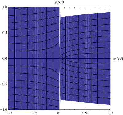
  • [40] Peng Cheng, Canli Song, Tong Zhang, Yanyi Zhang , Yilin Wang, Jin-Feng Jia, Jing Wang,Yayu Wang , Physical Review Letters 105, 076801 (2010)
  • [41] H.Peng et.al, Nature Materials ,9 225 -229 (2010)
  • [42] J.G.Analytis et al. cond/mat 1003.1713.
  • [43] R. Biswas and A.V. Balatsky, Phys.Rev.B 81, 23405 (2010).
  • [44] Ayelet Pnueli ‘J.Phys. A: Math.Gen.27 1345-1352 (1994)
  • [45] M.B.Green,J.H. Schwartz and E.Witten, ”‘Some Differential Geometry”’Superstrings Theory vol.2 Cambridge Monographs on Mathematical Physics pages 271−277271-277 (1987).
  • [46] N.D.Birrell and P.C. Davies ”‘Quantum Fields in Curved Space”’ pages 81−8581-85 Cambridge University Press (1982).
  • [47] Arnold M. Kosevici ”‘The Quantum Crystal”’ Wiley -VCH (2005).
  • [48] P. Di.Francesco. P. Mathieu and D. Senechal ”‘Conformal Field Theory”’ page 119, Springer Text in Contemporary Physics (1997).
  • [49] The Holomorphic representation of the delta function was brought to my attention by colleague V.P.Nair.
  • [50] P.Exner and P.Seba J.Math. Phys.30 2574-2580 (1989)
  • [51] J.Goldstone and R.L. Jaffe, Physical Review B45,14100(1992)
  • [52] R.C.T. da Costa,Physical Review A23,1982(1981)
  • [53] M.Maggiore, ”A Modern Introduction to Quantum Field Theory ”‘ Oxford University Press (2005),pages 2626-3131.