Cosmological solutions with massive gravitons
in the bigravity theory
Abstract
We present solutions describing homogeneous and isotropic cosmologies in the massive gravity theory with two dynamical metrics recently proposed in arXiv:1109.3515 and claimed to be ghost free. These solutions can be spatially open, closed, or flat, and at early times they are sourced by the perfect fluid, while the graviton mass typically manifests itself at late times by giving rise to a cosmological term. In addition, there are also exotic solutions, for which already at early times, when the matter density is high, the contribution of the graviton mass to the energy density is negative and large enough to screen that of the matter contribution. The total energy can then be negative, which may result in removing the initial singularity. For special parameter values there are also solutions for which the two metrics effectively decouple and evolve independently of each other. In the limit where one of the gravitational coupling constant vanishes, such special solutions reduce to those found in arXiv:1107.5504 within the theory where one of the metrics is flat.
I Introduction
The currently observed acceleration of our universe [1] is the main motivation of attempts to try to modify the theory of gravity, for example by giving a tiny mass to the graviton. This can effectively give rise to a small cosmological term leading to the late time acceleration [2]. The theory of massive gravity is not unique (see [3] for a review) and there exist a number of its models, typically parameterized by two metrics, one of which is physical, , while the other one is a flat reference metric . The coupling between the two is determined by a scalar function of .
Such models generically contain the negative norm ghost state in the spectrum [4]. There is, however, a particular model, we shall call it RGT model, that could be special, since it is the only one that is ghost-free in the decoupling limit [5]. In addition, this model was recently claimed to be ghost-free in the full theory [6]. Even though the possibility to have a completely ghost-free massive gravity is sometimes disputed [7], the RGT model is certainly interesting. Its solutions describing spatially closed, open and flat homogeneous and isotropic self-accelerating cosmologies were obtained in [8], [9].
Quite recently, the generalizations of the the GRT model were proposed, first by promoting the reference metric to be non-flat [10], and next promoting it to be dynamical [11], and it was argued that such generalized models remain ghost-free. In what follows we shall study the cosmological solutions within the bimetric theory of [11].
We find homogeneous and isotropic cosmologies which can be spatially open, closed, or flat. For the generic parameter values they can be of two main types. First of all, there are solutions for which the universe expansion is driven at early times by the ordinary matter, while the graviton mass manifests itself only at late times by giving rise to a cosmological term. In addition, there are also exotic solutions, for which already at early times, when the matter density is high, the contribution of the graviton mass to the energy density is large and negative and screens that of the matter contribution. The total energy can then be negative, which may result in removing the initial singularity. In addition, for special parameter values, we find solutions for which the two metrics evolve independently of each other and the physical metric shows the late time acceleration. In the limit where one of the gravitational coupling constant vanishes, we shall call it the RGT limit, they reduce to those of RGT theory found in [8]. It turns out that the generic solutions do not reduce in the GRT limit to any of the GRT theory, because both metrics remain then curved.
In what follows we present a rather detailed analysis of these solutions as well as their relation to the GRT limit. We address, in particular, the question (for some reason not discussed in the literature) of how to derive the Lagrangian field equations in the theory. This issue is in fact not as trivial as it may seem, since the interaction between the two metrics is parameterized by , whose direct variation is problematic, since the variation does not commute in the matrix sense with . We show how this problem can be handled withing the tetrad approach.
The rest of the paper is organized as follows. In Sec.II we describe the bimetric generalization of the RGT theory, the tetrad approach, the variation procedure and the reduction to the spherically symmetric sector. Solution with the decoupled metrics arising for special parameter values are described in Sec.III, while Sec.IV presents a detailed analysis of the generic case. Yet one more class of solutions, arising due to a different way to fulfill the conservation condition, is described in Sec.V, while the relation to the GRT limit is discussed in Sec.VI. We summarize our results in Sec.VII and list in the Appendix the energy-momentum tensor components.
II The bimetric generalization of the RGT model
The theory is defined on a four dimensional spacetime manifold parameterized by coordinates and equipped with two metrics and . Their kinetic terms are chosen to be of the standard Einstein-Hilbert form, with the corresponding couplings and . The dynamics is determined by the action
| (1) |
where and are the Ricci scalars for and , respectively, while describes ordinary matter (for example perfect fluid) which is supposed to interact only with . The interaction between the two metrics is defined by
| (2) |
with
| (3) |
where is defined by the relation
| (4) |
and is the inverse of . Apart from the gravitational coupling , the theory contains three parameters . In the limit where and is flat it reduces to the RGT theory [5].
The field equations are obtained by varying the action with respect to the metrics. A difficulty arises at this point, since varying the constraint (4) gives
| (5) |
and it is not obvious how to resolve this relation with respect to . One could of course consider as independent variables and impose the constraint (4) within the Lagrange multiplier method. However, the Lagrange multiplier enters then the equations as an auxiliary field, and it is unclear how to get rid of it. Therefore, we adopt a different strategy, motivated by the approach of [7], [8]. Let us introduce two tetrads and defined by the conditions
| (6) |
where is the Minkowski metric. We shall also need their inverse and such that and , similarly for . Each of the tetrads and is defined up to 6 local Lorentz rotation, so that equations (6) contain a 12-parameter gauge freedom. Let us now require that
| (7) |
where . This gives 6 local conditions, so that the two tetrads can now be Lorentz-rotated only simultaneously, which leaves only the 6-parameter freedom of local rotations in their definition. We then have a simple relation
| (8) |
because
| (9) |
which reproduces Eq.(4). As a result, we can vary the action with respect to and and the variation of will be obtained by varying Eq.(8). In order to take into account the conditions (7), we add to the Lagrangian the term
| (10) |
where are the 6 Lagrange multiplies. This allows us to consider and as independent variables. Performing then the variation and expressing from the resulting equations, we find that . Therefore, should be at the same time symmetric and antisymmetric on-shell, so that it should vanish.
As a result, we arrive at the following field equations
| (11) | ||||
| (12) |
where
| (13) |
with
| (14) | |||||
The Bianchi identities for the left-hand side of Eq.(11) imply the conservation condition
| (15) |
where is the covariant derivative with respect to . It is worth noting that the matter energy-momentum tensor is conserved independently, in view of the diffeomorphism-invariance of the matter action ,
| (16) |
The Bianchi identities for the left-hand side of Eq.(12) imply that , but these conditions in fact follow from Eq.(15), in view of the diffeomorphism-invariance of the interaction term . Indeed, let us consider a diffeomorphism induced by a vector field . It induces variations
| (17) |
while
| (18) | |||||
Since can be arbitrary, it follows that the conditions imply that .
If then the source term in (12) vanishes and one obtains , whose solution can be chosen to be flat metric, which can be written as , where are sometimes called Stuckelberg fields. All the above considerations then still apply, in particular the tetrad formalism, where it is sufficient to choose . The basic field equations are then (11),(15),(16) which determine and .
Let us return to the generic case with . In what follows we shall be considering solutions of equations (11), (12), (15), (16) with spherical symmetry. We introduce spherical coordinates and choose the tetrads to be
| (19) |
and
| (20) |
where are functions of . This implies the spherical symmetry for both metrics, while using the residual diffeomorphisms in the subspace one can always make the metric diagonal. We therefore set
| (21) |
so that . Next, we consider the symmetry conditions (7), of which the only non-trivial one is
| (22) |
from where . We then notice that changing the parameter corresponds to the simultaneous local Lorentz rotations of the two tetrads and does not change the metrics. We can therefore impose the gauge condition , which finally gives the following most general expressions for the tetrads:
| (23) |
The corresponding metrics read
| (24) |
and
| (25) |
while
| (26) |
and it is easy to verify that . We also notice that
| (27) |
We can now compute and the tensor defined by (14), they are shown in the Appendix. Since our fields are only SO(3)-invariant, we have at the time being , . Our aim is to find homogeneous and isotropic solutions for , in which case one should have and . We therefore proceed to eliminate the components and . One has
| (28) |
For this to vanish, we can either choose , or set to zero the expression between the parenthesis.
III Solutions with decoupled metrics
Let us first consider the case where and choose , where is a constant. Eq.(28) then becomes
| (29) |
which can be set to zero by adjusting the value of , but then one finds
| (30) |
which can in turn be set to zero by adjusting . It follows that setting
| (31) |
so that , one achieves both and . The components shown in the Appendix then reduce to
| (32) |
while
| (33) |
This gives
| (34) |
whereas using (27)
| (35) |
The field equations (11),(12) therefore become
| (36) | ||||
| (37) |
so that the equations for decouple from those for . It is now easy to get cosmological solutions. Setting
| (38) |
with , so that
| (39) |
and choosing , equations (36) reduce to
| (40) |
where is defined by the conservation condition
| (41) |
These equations describes the late time cosmological acceleration. If then so that for large the second term on the right in (40) becomes negligible. The dynamic is then driven by the cosmological term , which we assume to be positive, so that .
It is worth noting that Eq.(40) is exactly the same as Eq.(18) of [8] obtained in the RGT theory. These solutions therefore do not depend on weather the metric is dynamical or not, which is due to the fact that equations (36) for completely decouple from equations (37) for . In order to solve equations (37) for we notice that its components and are already fixed, since , but , , are still free, since they contain three up to now unspecified functions . To see that this freedom is enough to fulfill the ten equations (37), we notice that one can consider as the new radial coordinate. The time coordinate should also be changed, so that
| (42) |
and the metric becomes
| (43) |
where are functions of . The structure of the source term in (37) does not change in new coordinates, so that we should solve the Einstein equations with the negative cosmological term to find a metric parameterized by the radial Schwarzschild coordinate . The solution is the anti-de Sitter metric
| (44) |
where . One can now establish the relation to the coordinates, since we can read off the tetrad components from (44), but on the other hand they are given by (23), so that one can compare to obtain
| (45) |
This determines
| (46) |
and also
| (47) |
Together with , this establishes the correspondence between the and coordinates and also specifies all the unknown functions in the solution.
IV Generic solutions
Let us now return to Eq.(28) with arbitrary and set . This gives , while
We now choose both metrics to be homogeneous and isotropic,
| (48) |
This insures that the energy-momentum tensors depend only on time and have the diagonal structure, and (the explicit form of the tensor components can be read off from the formulas given in the Appendix). The independent equations are then the two Einstein equations
| (49) |
as well as the conservation condition for ,
| (50) |
One can check that the conservation condition for ,
| (51) |
gives exactly the same equation as (50), which shows once again that is identically conserved if is conserved.
The equation explicitly reads
| (52) | |||||
while the conservation condition
| (53) |
and the equation
| (54) | |||||
Let us set the second factor in (53) to zero,
| (55) |
thereby solving the conservation condition. Setting Eq.(52) reduces to
| (56) | |||||
while Eq.(54) becomes
| (57) | |||||
We see that the sources of the two metrics are proportional,
| (58) |
where fulfills the algebraic equation obtained by taking the difference of (56) and (57),
| (59) |
Since in view of the conservation condition (41), one therefore obtains . Injecting this to the right-hand side of Eq.(57) (or (56)) gives the source term , so that the solution can be determined.
Let us study roots of the quartic equation (59), first when . For there are generically two real roots, one of which is with , but depending on the parameter values there could be altogether four real roots. For example, for , and there are four roots with , respectively.
For non-zero there generically remain only two real roots, since the other two, if exist, merge to each other and disappear when increases. When , one of the two remaining roots is defined by
| (60) |
and the second one is
| (61) |
We shall say that the root (60) belongs to the physical branch, since is small and one can see from (56) that and because is small, so that . This is physically expected, since the graviton mass contribution to the total energy density should normally be small if the matter density is large. At the same time, these natural expectations do not apply to the root (61), since is then large and
| (62) |
so that the contribution of the graviton mass to the energy is as large as the matter contribution, and the two actually cancel each other, up to subleading terms. The resulting energy density
| (63) |
can even be negative, depending on the sign of . We therefore say that the root (61) belongs to the exotic branch.
Both the physical and exotic branches extend from large to small values of , so that they describe the decrease of during the universe expansion. When the universe is large and , the total energy approaches a constant value that can be positive or negative or zero, depending on the parameter values. For the physical branch is always positive and tends to zero as if , while for it approaches a positive value (for example, for , , ). For the exotic branch is positive/negative at large if is positive/negative, respectively, but it seems to always approach a non-zero negative value when (if ).
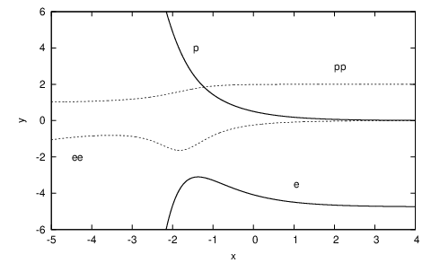
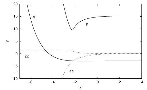
The described above different type behaviour of can be seen by solving the algebraic equation (59) numerically for different parameter values, as shown in Fig.1. One more type of solutions, shown in Fig.2 (left panel), is obtained by changing the sign of , in which case the sign of along the exotic branch changes from negative to positive values as decreases.
If then the coefficient in front of the highest power in Eq.(59) vanishes, so that there remain three roots. One finds in this case three different branches , these are the physical branch (60) and two exotic branches that start at large when one replaces (61) by
| (64) |
since there are two possibilities to choose the sign of when one takes the square root (these branches are called in Fig.2 exotic and exotic). If is large, then the energy for both exotic branches is the same up to subleading terms,
| (65) |
The behaviour of in the whole range of is shown in Fig.2 (right panel).
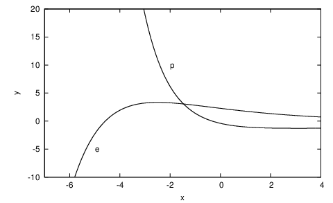
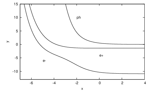
Now that we have determined , we can proceed to find solutions for the scale factor . Introducing the physical time , the Einstein equation (57) becomes
| (66) |
which describes a ‘particle’ with the total energy moving in the potential
| (67) |
Assuming a specific equation of state for the matter, the conservation condition (41) gives , which allows us to compute . In Fig.3 we show computed with the ultra-relativistic equation of state,
| (68) |
Solutions of Eq.(66) for a given correspond to the regions of where . Inspecting the curves in Fig.3 reveals then five different cases, of which the first two (in the left panel) correspond to the physical branches.
Type I solution correspond to the physical branches with for , in which case is negative and tends to zero as . The scale factor behaves qualitatively in the same way as in the matter dominated universe: it ranges in the finite limits in the spatially closed case , it linearly grows with for , and it increases as for .
Type II solutions correspond to the physical branches with (as for example in the right part of Fig.1). At early times they coincide with the ordinary matter-dominated cosmologies, since for the physical branches one has if is large. However, for large one has and , so that at late times solutions with enter the phase of accelerated expansion. For the things are slightly more subtle. The three curves IIa, IIb and IIc in Fig.3 correspond to different choices of the integration constant in (68). If is large (curve IIc) then and the solutions are similar to those with . If is small then the potential can exceed the value (curve IIa). Then there is a solution for which the ‘particle’ rests on the left of the reflection point (see Fig.3) close to the cosmological singularity , but there is also the solution that stays on the right of the reflection point (see Fig.3), it never approaches singularity and shows acceleration at large .
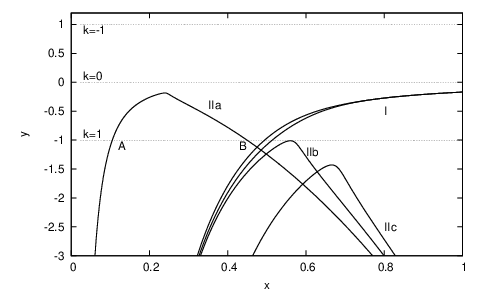
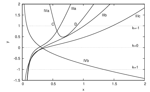
The exotic solutions are shown in the right part of Fig.3. Type III corresponds to exotic branches for which is positive at large but becomes negative when is small. The potential then grows from minus to plus infinity and the ‘particle’ is always confined to the region close to singularity. Type IV corresponds to the exotic branches for which is always negative, so that is unbounded from above but has a positive minimum. Solutions can exist only for and describe oscillations in the potential well between the two reflection points ( in Fig.3). Finally, type V corresponds to the exotic branch for for which changes from negative to positive values as decreases. The potential is then monotonically decreasing (see Fig.3) and the solutions always stay away from singularity and show the self-acceleration at large .
Summarizing, only types II and V show self-accelerating solutions. Type II solutions arise in theories with and , they evolve as the matter-dominated universe at early times, but enter the accelerated phase at late times. Type V solutions show late time acceleration, while at early times they are regular, being repelled from the singularity by the negative total energy . We notice, however, that such solutions require the second gravitational coupling constant to be negative.
V Non-accelerating solutions
Let us now return to the conservation equation (53) and try to fulfill it by setting to zero its first factor and not the second one. We therefore abandon the condition (55), but require instead that where is a constant. Then Eq.(53) will be satisfied if
| (69) |
Eq.(52) then reduces to
| (70) | |||||
while Eq.(54) becomes
| (71) |
Combining (70) and (71) one obtains
| (72) |
The quadratic equation (69) has two roots,
| (73) |
and the value of the cosmological constant in Eq.(70) is positive for one of them and negative for the other one. There is, however, an additional condition, since must be positive, and as the numerator in (72) is positive because , it follows that should be positive, since otherwise the denominator will become negative for large . Now, it turns out that if then , while if then . This eliminates solutions with , but there remain solutions with and , which exist if .
VI Limit
Let us first consider the solutions with decoupled metrics of Sec.III. Taking the limit does not affect the physical metric determined by Eqs.(39), (40), (41). On the other hand, the metric in (44) becomes flat, since when . One can write with and where and , while is obtained by settin in (47):
| (74) |
Equation (39),(40),(41),(74) exactly agree with Eqs.(16)–(18) obtained in [8] in the RGT limit. We therefore conclude that the solutions with decoupled metrics have the counterparts in the RGT theory, to which they approach when .
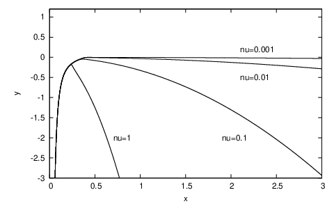
Let us now consider the generic solutions of Sec.IV. A direct inspection shows that does not necessarily become flat when , because the source term in Eq.(54) does not then vanish, neither does the source for the physical metric . To understand how this is possible, we notice that for the physical branches is small when is large, because (see Eq.(60)). On the other hand, Eq.(57) shows that when is small then for any . As a result, the effective potential does not vanish in the region where is small but approaches a non-trivial limit as (see Fig.4).
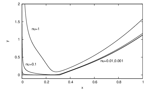
For some exotic branches becomes very small for small when , in which case one finds from (59) so that is independent of and the effective potential does not vanish at large . For other exotic branches never approaches zero, in which case as , therefore both and become flat. The conclusion is that the generic solutions of Sec.IV do not have non-trivial analogs in the RGT limit.
Finally, for the solutions of Sec.V the metric is determined by (69),(70) and does not depend on . The source term in (71) vanishes for and becomes flat. The limit is possible only for , since in (72) becomes ill-defined for if . As a result, the solutions of Sec.V do have, for , analogs in the RTG limit. Moreover, for one can choose in (70), as this no longer contradicts the positivity of in (72). Such solutions were found in [9], but only for they can be extended to .
We see that the bimetric theory admits solutions which do not approach for those of the theory, and vice versa, the theory has solutions which do not generalize for . One can construct more solutions for if we go directly to Eqs.(52),(53) and require that the metric parameterized by the functions (with ),
| (75) |
be flat. It will be flat if one finds such that
| (76) |
which is equivalent to three conditions
| (77) |
One possibility to fulfill these conditions is to set , , and
| (78) |
The conservation condition (53) is then fulfilled and one is left with the Einstein equation (52) where is constant. This reproduces the solutions given by Eqs.(19),(20) in [8] (the opposite sign convention for is used in [8]), they exist only in the RGT limit and do not generalize for .
Another possibility to fulfill (77) is to choose and set
| (79) |
With the conservation condition (53) is fulfilled if is given by (73), while is then determined by (70). The solutions were obtained in Ref.[9], they generalize to if only one chooses the root of (73) for which in (70) is negative.
Summarizing, among the accelerating solutions of the RGT theory only the special solutions (74) generalize for , while among accelerating solutions of the bimetric theory only solutions with the decoupled metrics of Sec.III have the RGT limit.
Recently it was claimed in the literature that the RTG theory does not actually admit homogeneous and isotropic cosmological solutions [12] (apart from those obtained in the decoupling limit [13]). At the same time, the presented above analysis shows very explicitly that such solutions exist, thus confirming the results of [8], [9]. The negative argument of [12] assumes that in the unitary gauge, where and , the physical metric is diagonal (see Eq.(13) in [12]). However, the two metrics cannot in general be diagonal at the same time. For example, is diagonal in coordinates , but with defined by formulas around Eq.(74) is not diagonal. For the solutions (78) both metrics are diagonal at the same time, but is degenerate, so that the argument of [12] again does not apply.
VII Summary
We have presented the homogeneous and isotropic cosmological solutions within the bimetric generalization of the RGT massive gravity theory. These solutions can be spatially open, closed, or flat, and at early times they are sourced by the perfect fluid, while the graviton mass typically manifests itself at late times by giving rise to a cosmological term whose value is determined by the theory parameters . In addition, there are also exotic solutions for which already at early times, when the matter density is high, the contribution of the graviton mass to the energy density is large and screens that of the matter contribution. The total energy can be negative, which can lead to non-singular solutions, as in the case of type II solutions with of Sec.IV. For type V solutions of Sec.IV the cosmological singularity is removed altogether, but this requires the second gravitational coupling to be negative.
In the limit where the second gravitational coupling tends to zero the generic solutions of Sec.IV do not reduce to solutions of the RGT theory, since both metrics remain then curved. However, the special solutions with decoupled metrics do have the non-trivial RGT limit.
The analysis of stability of our solutions remains an open issue to study. Since the graviton contribution to the total energy can be negative and very large for the exotic solutions, it is not impossible that the ghost could be still present in the theory, which may affect the stability.
APPENDIX
Here we list the energy momentum tensor components in the spherically symmetric case. Using the expression (26) for and computing gives the following value of the interaction Lagrangian (2):
| (A.1) | |||||
while the non-zero components of defined by Eq.(14) read
| (A.2) | |||||
| (A.3) | |||||
| (A.4) | |||||
| (A.5) |
The components of the two energy-momentum tensor are then simply obtained from Eq.(13), where is given by (27).
References
- [1] A.G. Reiss et al., Observational evidence from supernovae for an accelerating universe and a cosmological constant, Astron.J. 116 (1998) 1009; S. Perlmutter et al., Measurements of Omega and Lambda from 42 high redshift supernovae, Astrophys.J. 517 (1999) 565.
- [2] T. Damour, I.I. Kogan, A. Papazoglou, Nonlinear bigravity and cosmic acceleration, Phys.Rev. D66 (2002) 104025.
- [3] V.A. Rubakov, P.G. Tinyakov, Infrared-modified gravities and massive gravitons, Phys.Usp. 51 (2008) 759; K. Hinterbichler, Theoretical aspects of massive gravity, arXiv:1105.3735 [hep-th].
- [4] D.G. Boulware, S. Deser, Can gravitation have a finite range? Phys.Rev. D6 (1972) 3368.
- [5] C. de Rham, G. Gabadadze, A.J. Tolley, Resummation of massive gravity, Phys.Rev.Lett. 106 (2011) 231101. arXiv:1011.1232 [hep-th].
- [6] S.F. Hassan, R.A. Rosen, Resolving the ghost problem in non-linear massive gravity, arXiv:1106.3344 [hep-th].
- [7] A.H. Chamseddine, V. Mukhanov, Massive gravity simplified: a quadratic action, arXiv:1106.5868 [hep-th].
- [8] A.H. Chamseddine, M.S. Volkov, Cosmological solutions with massive gravitons Phys.Lett. B704 (2011) 652. arXiv:1107.5504 [hep-th].
- [9] A.E. Gumrukcuoglu, C. Lin, S. Mukohyama, Open FRW universes and self-acceleration from nonlinear massive gravity, arXiv:1109.3845 [hep-th].
- [10] S.F. Hassan, R.A. Rosen, A.Schmidt-May, Ghost-free massive gravity with a general reference metric, arXiv:1109.3230 [hep-th].
- [11] S.F. Hassan, R.A. Rosen, Bimetric gravity from ghost-free massive gravity, arXiv:1109.3515 [hep-th].
- [12] G.D’Amico, C. de Rham, S. Dubovsky, G. Gabadadze, D. Pirtskhalava, A.J. Tolley, Massive cosmologies, arXiv:1108.5231 [hep-th].
- [13] C. de Rham, G. Gabadadze, A.J. Tolley, Cosmic acceleration and the helicity-0 Graviton, Phys.Rev. D83 (2011) 103516. arXiv:1010.1780 [hep-th]; K. Koyama, G. Niz, G. Tasinato, The self-accelerating universe with vectors in massive gravity. arXiv:1110.2618 [hep-th].