Quark number susceptibility at finite density and low temperature
Abstract:
We study the quark number susceptibility in SU(2) lattice gauge theory with two Wilson quark flavours at non-zero chemical potential and low temperature. We present some technical aspects of the issue and numerical results obtained at different lattices and different parameters. We discuss what this observable can teach us about the phase diagram of the model and in particular about the relation between susceptibility and Polyakov loop.
July 10 - 16, 2011
Squaw Valley, Lake Tahoe, California
1 Introduction
Studying the statistical fluctuations of a system is a powerful method to characterise the thermodynamic properties of a system. As a matter of fact, the presence of a phase transition is signalled by an enhancement of the fluctuations in the system. The observables appropriate to extract this kind of information are called susceptibilities. Properly, the susceptibility describes the response of a system to an applied field. Given an operator we can usually determine a corresponding susceptibility that is the second derivative of the free energy density. In this paper we are interested in studying the quark number susceptibility (QNS) : it is the response of , the quark number density, to an infinitesimal change in the quark chemical potential .
The QNS has been studied so far at finite temperature and zero chemical potential, see Refs. [1, 2, 3]. This is largely because QNS is directly related to experimental measurements of fluctuations observed in heavy ion collisions [4]. At non-zero density and zero (or low) temperature regime, QNS is not commonly studied; an application to QCD of rainbow approximation of the Dyson-Schwinger approach to study the QNS can be found in Ref. [5]. One reason for the lack of studies in this regime is the well known sign problem: it is not possible, using standard tools, to simulate lattice QCD at non-zero density.
In this paper we study the QNS at non-zero density and at low temperature in the context of gauge theory, i.e. where simulations are feasible.
2 Two color QCD
In two color QCD, i.e. gauge theory, quarks and antiquarks live in equivalent representations of the group; the physical consequence is that mesons and , baryons are contained in the same hadron multiplet. In the limit when , i.e. when the pion mass is very small compared with the first non-Goldstone hadron, it is possible to study the system using the chiral perturbation theory (PT) limit [6]. The fundamental result is that only for the quark number density becomes different from zero and at the same onset value also a condensate develops, signalling the spontaneous breakdown of the global baryon number symmetry: a superfluid phase appears. In this phase there are tightly bound scalar diquarks but the hadrons are weakly interacting between them: therefore, just above the onset, the system is very dilute and is described as a Bose Einstein Condensate (BEC).
Using PT it is possible to determine the behaviour of different observables; in particular, we can write down the prediction for and its susceptibility , at zero temperature and in the limit (right-hand limit):
| (1) |
where is the pion decay constant and the number of fermions. The diquark condensate, calculated in the same limits, is given in terms of the chiral condensate at zero chemical potential:
| (2) |
There are reasons to think that above a certain value of the chemical potential, , a degenerate system of weakly interacting quarks is more stable [7]. For an ideal gas (Stefan Boltzmann (SB) limit) of massless quarks and gluons, at , we have:
| (3) |
where is the number of colours. In this case the superfluidity is explained by a BCS condensation of Cooper pairs within a layer of thickness around the Fermi surface; the diquark condensate is therefore given by:
| (4) |
Comparing Eq.s (1), (2) with Eq.s (3), (4), we see clearly that the two phases are characterised by two quite different behaviours.
We consider also the order parameter related to the confinement property of the theory: the Polyakov loop ; as discussed in Ref. [8] the theory becomes deconfined only after . Surprisingly, there is a regime, , where the theory is confined, i.e. , but the other observables seem to suggest non interacting fermions: a confined BCS phase. This phase could be the so called quarkyonic phase introduced in Ref. [9]; arguments against the extension of this idea to the case of can be found in Ref.[10].
3 Calculation of the observables
The fermion action with and with a diquark source term , necessary to study the diquark condensate, is given by:
| (5) |
where is the standard Wilson fermion matrix at non-zero chemical potential and is the charge conjugation operator. If we introduce the change of variables , , , , it is possible to rewrite the action as:
| (6) |
It is worth mentioning that , therefore we can take the square root analytically, i.e. there is no square root problem. The partition function becomes:
| (7) |
It is now easy to write down an expression for using the matrix :
| (8) |
Moreover, from the definition of QNS we have:
| (9) |
From this equation we can identify four different terms:
| (10) | |||||
| (11) | |||||
| (12) | |||||
| (13) |
We see that from the second term of Eq. (9) we get two terms, namely and , because there are two ways to contract the spinors.
The calculation of the traces is done by unbiased estimators, introducing complex noise vectors with the properties: and . For example, the determination of the following trace, used for and , is based on the relation:
| (14) |
Because for we need two independent source vectors we refer to this term as disconnected term; the other three terms need only one source vector and we call them connected terms.
4 Some numerical issues
The source vector used to determine the traces can characterised by different noise distributions. The standard method is based on the introduction of gaussian complex noise vector but it is possible also to use a complex noise vector (see Ref. [11] where the potential advantage are discussed). In the case, the complex noise vectors takes one of the four values , chosen independently with equal probability.
In Table 1 we present an example where we used only three noise vectors, with the following parameters: , , , , .
| T1 | T2 | T3 | C1 | ||
|---|---|---|---|---|---|
| Gaussian | 2.25(8.30)E-06 | 5.00(5.74)E-05 | 0.4010(27) | -0.3681(107) | 3.1(1.0) |
| 6.3(10.0)E-06 | 7.4(49.9)E-06 | 0.3994(32) | -0.3655(66) | 3.17(52) |
From this simple analysis, we can see that there is no any particular advantage in using a noise, so in the following we continue to use only gaussian noise distributions.
We also tried to see what happen when we increase the number of noise vectors; in Table 2 we present an example with the same parameters used above.
| noise vectors | T1 | T2 | T3 | C1 | |
|---|---|---|---|---|---|
| 3 | 2.25(8.30)E-06 | 5.00(5.74)E-05 | 0.4010(27) | -0.3681(107) | 3.1(1.0) |
| 300 | 1.50(17)E-05 | 1.53(12)E-05 | 0.4013(14) | -0.3612(20) | 4.04(11)E-02 |
From this result it is evident how increasing the number of noise vectors has a strong effect mainly on observables with a small value; the effect is very limited if the observable is clearly different from zero.
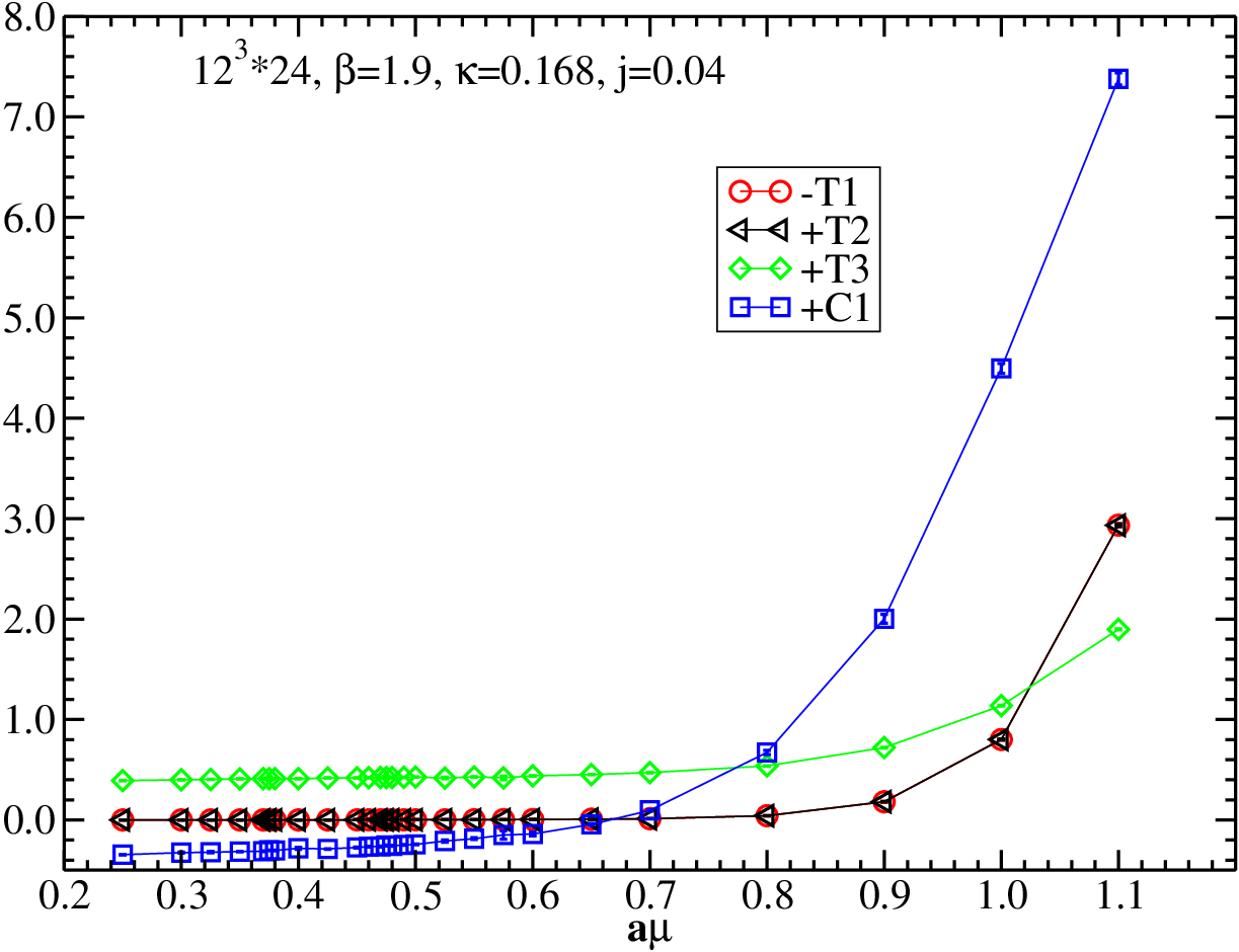

In Fig. 1 (Left) we plot the four terms (note the sign of ) vs the chemical potential. The connected contribution gives clearly an important contribution either at low and high values of the chemical potential; note the changing of sign around . The terms and are equal in magnitude but with opposite sign, therefore their contribution cancels everywhere, Fig. 1 (Right); in other words the variance of the quantity in Eq. (14) is equal to zero. We see very strong fluctuations, apparently not compatible with one, for , then smoothed fluctuations comparable with one until and after this a stable ratio equal to one.
5 Numerical results
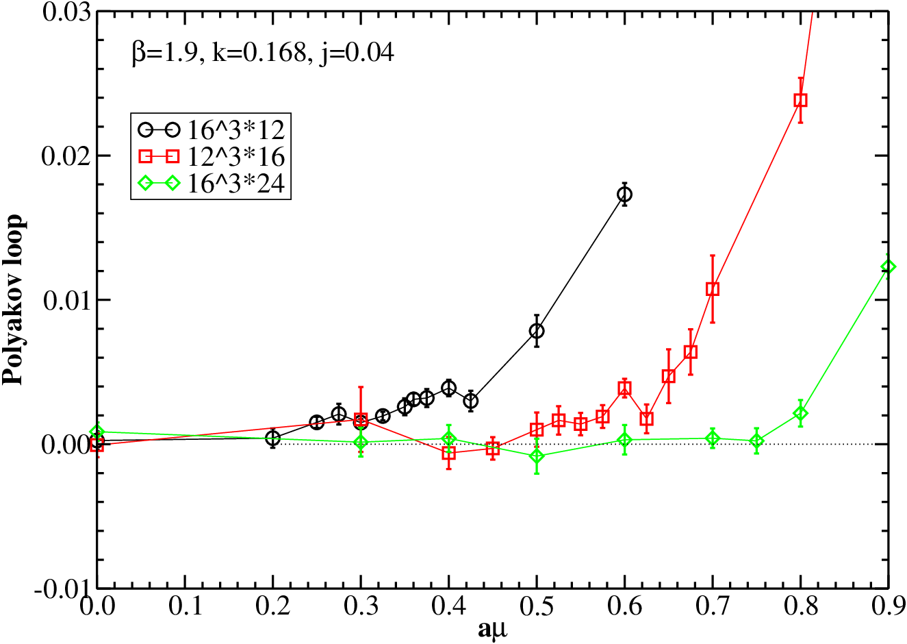
In this contribution we are going to show some results obtained for and . From previous works, see Ref. [8] and the references therein, we know that for these parameters , therefore ; moreover, there are signals of a BEC phase for .
We obtained interesting results comparing the QNS with the other observables; here we want to stress an interesting effect we have observed studying the system at different temperatures. Note that the results we are presenting should eventually be extrapolated to .
In Fig. 2 (Left) we plot the ratio , for three different temperatures, versus the chemical potential. For an ideal gas of quarks this ratio would be a constant, see Eq. (3), and we see that a plateau is actually present for ; after this value we can see a sharp increase of the QNS. Moreover, it is evident from this plot that the QNS is quite independent from the temperature, i.e. we do not see any drastic deviations in the behaviour of the three curves increasing . This is in contrast with the Polyakov loop behaviour that shows deconfinement for three different values of the chemical potential, correspondingly at the three different temperatures, Fig. 2 (Right).

It is instructive to compare our lattice numerical results with the equations corresponding to Eq. (3) but taking in account the finite volume and the lattice discretisation. In Ref. [7], see Eq. (26), the expression for the quark number density for free Wilson fermions on the lattice is presented. It is then easy to obtain .
In Fig. 3 we plot the ratio between the measured QNS and for two values of the fermion mass: in the determination of we have to fix a value for the mass of the free fermion; unfortunately we do not know this value, therefore we consider massless fermions (note that this is the same limit used in Eq. (3)) and a value of the order of . In this case we observe a different behaviour for , reminiscent of the BEC phase, followed by a flat region compatible with ratio one, i.e. the system is behaving as free fermions, and then again we see an increase for higher values of . These plots again confirm the above scenario: we do not see any abrupt change for QNS, for any of the values of , where instead the Polyakov loop becomes different from zero.
Note that the QNS is often taken as an alternative signal for deconfinement in lattice studies of the thermal QCD transition i.e. there is a strong connection between and Polyakov Loop, see Refs. [12, 13, 14]. Our results shows that this relation is not replicated at low temperature and high density.


6 Conclusion
In this work we have studied the quark number susceptibility at non-zero density and low temperature in the case of two color QCD with two flavours. We have studied the contribution of the different terms, connected and disconnected, which contribute to it and finally we have shown its behavior at finite temperature. Surprisingly, we have seen that in this case there is no relation between the quark number susceptibility and the Polyakov loop, i.e. in this context it cannot be used as a signal for deconfinement as it is usually done at finite temperature and zero quark number density. This observation could suggest that the deconfinement transition is not characterised by a liberation of additional degrees of freedom; if this phenomenon is exclusive to two color QCD or related to the non small ratio or, somehow, connected to the presence of a quarkyonic phase, is under study. Clearly, there is much to learn about deconfinement from studying a new physical environment.
References
- [1] S. A. Gottlieb, W. Liu, D. Toussaint, R. L. Renken, R. L. Sugar, Phys. Rev. Lett. 59 (1987) 2247.
- [2] C. R. Allton, M. Doring, S. Ejiri, S. J. Hands, O. Kaczmarek, F. Karsch, E. Laermann, K. Redlich, Phys. Rev. D71 (2005) 054508. [hep-lat/0501030].
- [3] R. V. Gavai, S. Gupta, Phys. Rev. D78 (2008) 114503. [arXiv:0806.2233 [hep-lat]].
- [4] M. Asakawa, U. W. Heinz, B. Muller, Phys. Rev. Lett. 85 (2000) 2072-2075. [hep-ph/0003169].
- [5] D. -K. He, Y. Jiang, H. -T. Feng, W. -M. Sun, H. -S. Zong, Chin. Phys. Lett. 25 (2008) 440-443.
- [6] J. B. Kogut, M. A. Stephanov, D. Toublan, J. J. M. Verbaarschot, A. Zhitnitsky, Nucl. Phys. B582 (2000) 477-513. [hep-ph/0001171].
- [7] S. Hands, S. Kim, J. -I. Skullerud, Eur. Phys. J. C48 (2006) 193. [hep-lat/0604004].
- [8] S. Hands, S. Kim, J. -I. Skullerud, Phys. Rev. D81 (2010) 091502. [arXiv:1001.1682 [hep-lat]].
- [9] L. McLerran, R. D. Pisarski, Nucl. Phys. A796 (2007) 83-100. [arXiv:0706.2191 [hep-ph]].
- [10] S. Lottini, G. Torrieri, accepted for publication in Phys. Rev. Lett. on Sep 08, 2011. [arXiv:1103.4824 [nucl-th]].
- [11] S. -J. Dong, K. -F. Liu, Phys. Lett. B328 (1994) 130-136. [hep-lat/9308015].
- [12] Y. Aoki, Z. Fodor, S. D. Katz, K. K. Szabo, Phys. Lett. B643 (2006) 46-54. [hep-lat/0609068].
- [13] A. Bazavov, T. Bhattacharya, M. Cheng, N. H. Christ, C. DeTar, S. Ejiri, S. Gottlieb, R. Gupta et al., Phys. Rev. D80 (2009) 014504. [arXiv:0903.4379 [hep-lat]].
- [14] S. Hands, T. J. Hollowood, J. C. Myers, JHEP 1012 (2010) 057. [arXiv:1010.0790 [hep-lat]].