\pkglgcp – An \proglangR Package for Inference with Spatio-Temporal Log-Gaussian Cox Processes

Benjamin M. Taylor
Lancaster University UK Tilman M. Davies
Massey University NZ Barry S. Rowlingson
Lancaster University UK Peter J. Diggle
Lancaster University UK Email: b.taylor1@lancaster.ac.uk Email: T.Davies@massey.ac.nz Email: b.rowlingson@lancaster.ac.uk Email: p.diggle@lancaster.ac.uk

\Plainauthor

Benjamin M. Taylor, Tilman M. Davies, Barry S. Rowlingson, Peter J. Diggle \Plaintitlelgcp – An R Package for Inference with Spatio-Temporal Log-Gaussian Cox Processes \AbstractThis paper introduces an \proglangR package for spatio-temporal prediction and forecasting for log-Gaussian Cox processes. The main computational tool for these models is Markov chain Monte Carlo and the new package, \pkglgcp, therefore also provides an extensible suite of functions for implementing MCMC algorithms for processes of this type. The modelling framework and details of inferential procedures are first presented before a tour of \pkglgcp functionality is given via a walk-through data-analysis. Topics covered include reading in and converting data, estimation of the key components and parameters of the model, specifying output and simulation quantities, computation of Monte Carlo expectations, post-processing and simulation of data sets. \KeywordsCox process; \proglangR; spatio-temporal point process \Plainkeywordsspatio-temporal point processes, R \AddressBenjamin M. Taylor
Division of Medicine,
Lancaster University,
Lancaster,
LA1 4YF,
UK
E-mail:
URL: http://www.maths.lancs.ac.uk/~taylorb1/ Tilman M. Davies
Institute of Fundamental Sciences
Massey University
Science Tower ScB2.10
Manawatu Campus
Private Bag 11222
Palmerston North 4442
New Zealand
E-mail:
URL: http://ifs.massey.ac.nz/people/staff.php?personID=232 Barry Rowlingson
Division of Medicine,
Lancaster University,
Lancaster,
LA1 4YF,
UK
E-mail:
URL: http://www.maths.lancs.ac.uk/~rowlings/ Professor Peter J. Diggle
Division of Medicine,
Lancaster University,
Lancaster,
LA1 4YF,
UK
E-mail:
URL: http://www.lancs.ac.uk/~diggle/

1 Introduction

This article introduces a new \proglangR package, \pkglgcp, for inference with spatio-temporal log-Gaussian Cox processes \proglangR Development Core Team (2011). The work was motivated by applications in disease surveillance, where the major focus of scientific interest is on whether, and if so where and when, cases form unexplained clusters within a spatial region $W$ and time-interval $(0,T)$ of interest. It will be assumed that both the location and time of each case is known, at least to a sufficiently fine resolution that a point process modelling framework is natural. In general, the aims of statistical analysis include model formulation, parameter estimation and spatio-temporal prediction. The \pkglgcp package includes some functionality for parameter estimation and diagnostic checking, mostly by linkages with other \proglangR packages for spatial statistics. However, and consistent with the scientific focus being on disease surveillance, the current version of the package places particular emphasis on real-time predictive inference. Specifically, using the modelling framework of a Cox process with stochastic intensity $R(x,t)=\exp\{{\mathcal{Y}}(x,t)\}$ , where ${\mathcal{Y}}(x,t)$ is a Gaussian process, the package enables the user to draw samples from the joint predictive distribution of $R(x,t+k)$ given data up to and including time $t\leq T$ , for any set of locations $x\in W$ and forecast lead time $k\geq 0$ . In the surveillance setting, these samples would typically be used to evaluate the predictive probability that the intensity at a particular location and time exceeds a specified intervention threshold; see, for example, Diggle et al. (2005).

The \pkglgcp package makes extensive use of \pkgspatstat functions and data structures (Baddeley and Turner, 2005). Other important dependencies are: the \pkgsp package, which also supplies some data structures and functions (Pebesma and Bivand, 2005; Bivand et al., 2008); the suite of covariance functions provided by the \pkgRandomFields package (Schlather, 2001); the \pkgrpanel package to facilitate minimum-contrast parameter estimation routines (Bowman et al., 2007; Bowman et al., 2010); and the \pkgncdf package for rapid access to massive datasets for post-processing (Pierce, 2011).

In Section 2 the log-Gaussian Cox process is introduced. Section 3 gives a review on methods of inference for log-Gaussian Cox processes. Section 4 is an overview of the package by way of a walk-through example, covering: reading in data (Section 4.1); estimating components of the model and associated parameters (Sections 4.2 and 4.3); setting up and running the model (Sections 4.4 and 4.5); and post-processing of command outputs (Section 4.6). Some possible extensions of the package are given in Section 5. The appendices give further information on the rotation of observation windows (Appendix A), simulation of data (Appendix B) and information about the \codespatialAtRisk class of objects (Appendix C), which may be useful for reference purposes.

2 Spatio-Temporal log-Gaussian Cox processes

Let $W\subset\mathbb{R}^{2}$ be an observation window in space and $T\subset\mathbb{R}_{\geq 0}$ be an interval of time of interest. Cases occur at spatio-temporal positions $(x,t)\in W\times T$ according to an inhomogeneous spatio-temporal Cox process, i.e., a Poisson process with a stochastic intensity $R(x,t)$ . The number of cases, $X_{S,[t_{1},t_{2}]}$ , arising in any $S\subseteq W$ during the interval $[t_{1},t_{2}]\subseteq T$ is then Poisson distributed conditional on $R$ ,

X_{S,[t_{1},t_{2}]}\sim\text{Poisson}\left\{\int_{S}\int_{t_{1}}^{t_{2}}R(s,t)\mathrm{d}s\mathrm{d}t\right\}.

(1)

Following Diggle et al. (2005), the intensity is decomposed multiplicatively as,

R(s,t)=\lambda(s)\mu(t)\exp\{\mathcal{Y}(s,t)\}.

(2)

In Equation 2,the fixed spatial component, $\lambda:\mathbb{R}^{2}\mapsto\mathbb{R}_{\geq 0}$ , is a known function, proportional to the population at risk at each point in space and scaled so that,

\int_{W}\lambda(s)\mathrm{d}s=1,

(3)

whilst the fixed temporal component, $\mu:\mathbb{R}_{\geq 0}\mapsto\mathbb{R}_{\geq 0}$ , is also a known function such that,

\mu(t)=\lim_{\delta t\rightarrow 0}\left\{\frac{\E[X_{W,\delta t}]}{|\delta t|}\right\}.

(4)

The function $\mathcal{Y}$ is a Gaussian process, continuous in both space and time. In the nomenclature of epidemiology, the components $\lambda$ and $\mu$ determine the endemic spatial and temporal component of the population at risk; whereas $\mathcal{Y}$ captures the residual variation, or the epidemic component.

The Gaussian process, $\mathcal{Y}$ , is second order stationary with minimally-parametrised covariance function,

\mathrm{cov}[\mathcal{Y}(s_{1},t_{1}),\mathcal{Y}(s_{2},t_{2})]=\sigma^{2}r(||s_{2}-s_{1}||;\phi)\exp\{-\theta(t_{2}-t_{1})\},

(5)

where $||\,\cdot\,||$ is a suitable norm on $\mathbb{R}^{2}$ , for instance the Euclidean norm, and $\sigma,\phi,\theta>0$ are known parameters. In the \pkglgcp package, the isotropic spatial correlation function, $r$ , may take one of several forms and possibly require additional parameters (in \pkglgcp, this can be selected from any of the compatible models in the function \codeCovarianceFct from the \pkgRandomFields package). The parameter $\sigma$ scales the log-intensity, whilst the parameters $\phi$ and $\theta$ govern the rates at which the correlation function decreases in space and in time, respectively. The mean of the process $\mathcal{Y}$ is set equal to $-\sigma^{2}/2$ so as to give $\E[\exp\{\mathcal{Y}\}]=1$ , hence the endemic/epidemic analogy above.

3 Inference

As in Møller et al. (1998), Brix and Diggle (2001) and Diggle et al. (2005), a discretised version of the above model will be considered, defined on a regular grid over space and time. Observations, $X$ , are then treated as cell counts on this grid. The discrete version of $\mathcal{Y}$ will be denoted $Y$ ; since $Y$ is a finite collection of random variables, the properties of $\mathcal{Y}$ imply that $Y$ has a multivariate Gaussian density with approximate covariance matrix $\Sigma$ , whose elements are calculated by evaluating Equation 5 at the centroids of the spatio-temporal grid cells. Without loss of generality, unit time-increments are assumed and events can be thought of as occurring “at” integer times $t$ . Let $X_{t}$ denote an observation over the spatial grid at time $t$ , and $X_{t_{1}:t_{2}}$ denote the observations at times $t_{1},t_{1}+1,\ldots,t_{2}$ . For predictive inference about $Y$ , samples from the conditional distribution of the latent field, $Y_{t}$ , given the observations to date, $X_{1:t}$ would be drawn, but this is infeasible because the dimensionality of the required integration increases without limit as time progresses. An alternative, as suggested by Brix and Diggle (2001), is to sample from $Y_{t_{1}:t_{2}}$ given $X_{t_{1}:t_{2}}$ ,

\pi(Y_{t_{1}:t_{2}}|X_{t_{1}:t_{2}})\propto\pi(X_{t_{1}:t_{2}}|Y_{t_{1}:t_{2}})\pi(Y_{t_{1}:t_{2}}),

(6)

where $t_{1}=t_{2}-p$ for some small positive integer $p$ . The justification for this approach is that observations from the remote past have a negligible effect on inference for the current state, $Y_{t}$ .

In order to evaluate $\pi(Y_{t_{1}:t_{2}})$ in Equation 6, the parameters of the process $Y$ must either be known or estimated from the data. Estimation of $\sigma$ , $\phi$ and $\theta$ may be achieved either in a Bayesian framework, or by one of a number of more ad hoc methods. The methods implemented in the current version of the \pkglgcp package fall into the latter category and are described in Brix and Diggle (2001) and Diggle et al. (2005). Briefly, this involves matching empirical and theoretical estimates of the second-moment properties of the model. For the spatial covariance parameters $\sigma$ and $\phi$ , the inhomogeneous $K$ -function, or $g$ function are used (Baddeley et al., 2000). The autocorrelation function of the total event-counts per unit time-interval is used for estimating the temporal correlation parameter $\theta$ . The estimated parameter values can then be used to implement plug-in-prediction for the latent field $Y_{t}$ .

3.1 Discretising and the fast-Fourier transform

The first barrier to inference is computation of the covariance matrix, $\Sigma$ , which even for relatively coarse grids is very large. Fortunately, for regular spatial grids of size $2^{m}\times 2^{n}$ , there exist fast methods for computing this based on the discrete Fourier transform (Wood and Chan, 1994). The general idea is to embed $\Sigma$ in a symmetric circulant matrix, $C=Q\Lambda Q^{*}$ , where $\Lambda$ is a diagonal matrix of eigenvalues of $C$ , $Q$ is a unitary matrix and ^∗ denotes the Hermitian transpose. The entries of $Q$ are given by the discrete Fourier transform. Computation of $C^{1/2}$ , which is useful for both simulation and evaluation of the density of $Y$ , is then straightforward using the fact that $C^{1/2}=Q\Lambda^{1/2}Q^{*}$ .

3.2 The Metropolis-adjusted Langevin algorithm

Monte Carlo simulation from $\pi(Y_{t_{1}:t_{2}}|X_{t_{1}:t_{2}})$ is made more efficient by working with a linear transformation of $Y$ , partially determined by the matrix $C$ as described below. The \pkglgcp package returns results pertaining to $Y$ on a grid of size $M\times N\equiv 2^{m}\times 2^{n}$ for positive integers $m$ and $n$ specified by the user, which is extended to a grid of size $2M\times 2N$ for computation (Møller et al., 1998). Writing $\Gamma_{t}=\Lambda^{-1/2}Q(Y_{t}-\mu)$ , the target of interest is given by,

\pi(\Gamma_{t_{1}:t_{2}}|X_{t_{1}:t_{2}})\propto\left[\prod_{t=t_{1}}^{t_{2}}\pi(X_{t}|Y_{t})\right]\left[\pi(\Gamma_{t_{1}})\prod_{t=t_{1}+1}^{t_{2}}\pi(\Gamma_{t}|\Gamma_{t-1})\right],

(7)

where the first term on the right hand side of Equation 7 corresponds to the first bracketed term on the right hand side of Equation 6 and the second bracketed term is the joint density, $\log\{\pi(\Gamma_{t_{1}:t_{2}})\}$ . Because $\Gamma$ is an Ornstein-Uhlenbeck process in time, the transition density, $\pi(\Gamma_{t}|\Gamma_{t-1})$ , has an explicit expression as a Gaussian density; see Brix and Diggle (2001).

Since the gradient of the transition density can also be written down explicitly, a natural and efficient MCMC method for sampling from the predictive density of interest (Equation 7), is a Metropolis-Hastings algorithm with a Langevin-type proposal (Roberts and Tweedie, 1996),

q(\Gamma,\Gamma^{\prime})=\mathrm{N}\left[\Gamma^{\prime};\Gamma+\frac{1}{2}\nabla\log\{\pi(\Gamma|X)\},h^{2}\mathbb{I}\right],

where $\mathrm{N}(y;m,v)$ denotes a Gaussian density with mean $m$ and variance $v$ evaluated at $y$ , $\mathbb{I}$ is the identity matrix and $h>0$ is a scaling parameter (Metropolis et al., 1953; Hastings, 1970).

Various theoretical results exist concerning the optimal acceptance probability of the MALA (Metropolis-Adjusted Langevin Algorithm) – see Roberts and Rosenthal (1998) and Roberts and Rosenthal (2001) for example. In practical applications, the target acceptance probability is often set to 0.574, which would be approximately optimal for a Gaussian target as the dimension of the problem tends to infinity. An algorithm for the automatic choice of $h$ , so that this acceptance probability is achieved without disturbing the ergodic property of the chain, is also straightforward to implement, see Andrieu and Thoms (2008).

4 Introducing the \pkglgcp package

4.1 Reading-in and converting data

The generic data-format of interest is $(x_{i},y_{i},t_{i}):i=1,...,n$ , where the $(x_{i},y_{i})$ are the locations and $t_{i}$ the times of occurrence of events in $W\times(A,B)$ , where W is a polygonal observation window and $(A,B)$ the time-interval within which events are observed. In the following example \codex, \codey and \codet are \proglangR objects giving the location and time of events and \codewin is a \pkgspatstat object of class \codeowin specifying the polygonal observation window (Baddeley and Turner, 2005). An example of constructing an appropriate \codeowin object from ESRI shapefiles is given in the package vignette (type \codevignette("lgcp")).

{CodeChunk}{CodeInput}

R> data <- cbind(x,y,t) R> tlim <- c(0,100) R> win {CodeOutput} window: polygonal boundary enclosing rectangle: [381.7342, 509.7342] x [64.14505, 192.14505] units

The first task for the user is to convert this into a space-time planar point pattern object ie. one of class \codestppp, provided by \pkglgcp. An object of class \codestppp is easily created: {CodeChunk} {CodeInput} R> xyt <- stppp(list(data=data,tlim=tlim,window=win)) R> xyt {CodeOutput} Space-time point pattern planar point pattern: 10069 points window: polygonal boundary enclosing rectangle: [381.7342, 509.7342] x [64.14505, 192.14505] units Time Window : [ 0 , 100 ]

4.2 Estimating the spatial and temporal component

There are many ways to estimate the fixed spatial and temporal components of the log-Gaussian Cox process. The fixed spatial component, $\lambda(s)$ , represents the spatial intensity of events, averaged over time and scaled to integrate to 1 over the observation window $W$ . In epidemiological settings, this typically corresponds to the spatial distribution of the population at risk, although this information may not be directly available. The fixed temporal component, $\mu(t)$ , is the mean number of events in $W$ per unit time. Where the relevant demographic information is unavailable to specify $\lambda(s)$ and $\mu(t)$ directly, \pkglgcp provides basic functionality to estimate them from the data.

The function \codelambdaEst is an interactive implementation of a kernel method for estimating $\lambda(s)$ as in the following example: {CodeChunk} {CodeInput} R> den <- lambdaEst(xyt,axes=TRUE) R> plot(den) This calls an \pkgrpanel tool (Bowman et al., 2007) for estimating $\lambda$ (see Figure 1); once the user is happy with the result, clicking on “OK” closes the panel and the kernel density estimate is stored in the \proglangR object \codeden of class \codeim (a \pkgspatstat pixel image object). The estimate of $\lambda$ can then be plotted in the usual way. The parameters \codebandwidth and \codeadjust in this GUI relate to the arguments from the \pkgspatstat function \codedensity.ppp; the former corresponds to the argument \codesigma and the latter to the argument of the same name.

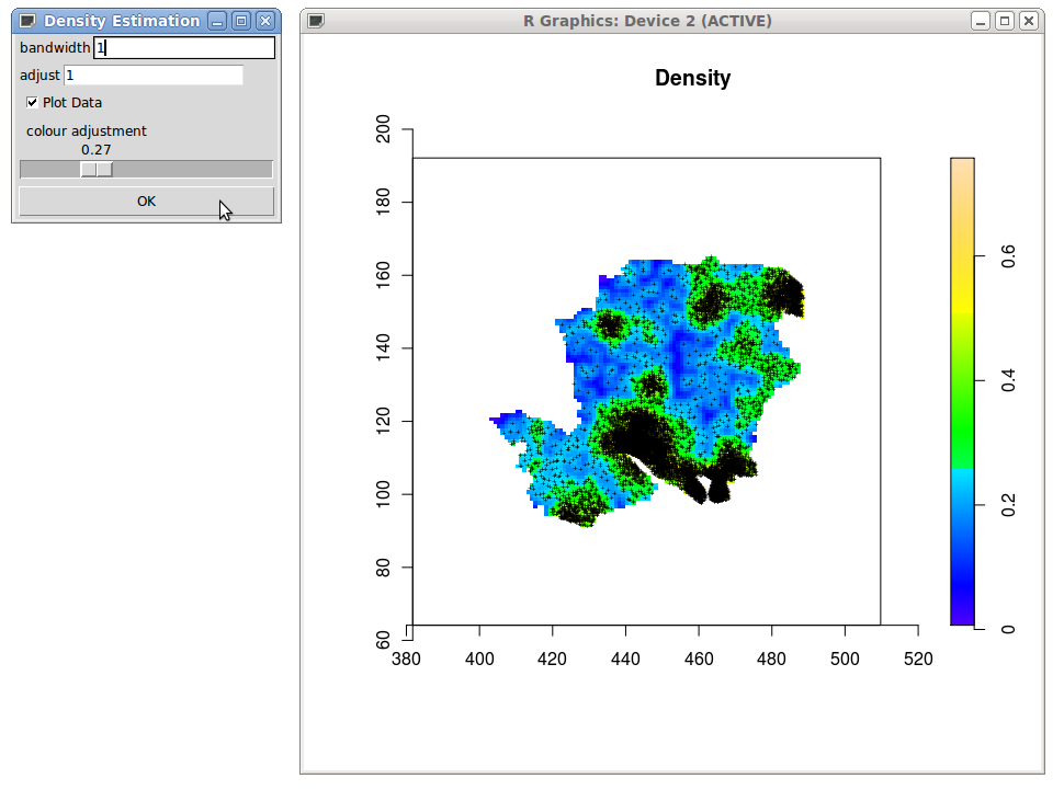
Refer to caption — Figure 1: Choosing a kernel density estimate of $\lambda(s)$ .

The \pkglgcp package provides methods for coercing pixel-images like \codeden to objects of class \codespatialAtRisk, which can then be used in parameter estimation and in the MALA algorithm to be discussed later; further useful information on the \codespatialAtRisk class is provided in Appendix C. {CodeChunk} {CodeInput} R> sar <- spatialAtRisk(den) {CodeOutput} SpatialAtRisk object X range : [382.3742066569,509.094206656898] Y range : [64.785045372051,191.505045372051] dim : 100 x 100 For the temporal component, $\mu(t)$ , the user must provide an object that can be coerced into one of class \codetemporalAtRisk.

Objects of class \codetemporalAtRisk are non-negative functions of time over an observation time-window of interest, which must be the same as the time-window of the \codestppp data object, \codexyt. In some applications (Diggle et al., 2005), $\mu(t)$ might represent the fitted values of a parametric model for the case counts over time. As it is not possible to provide generic functionality for parametric $\mu(t)$ , a simple non-parametric estimate of $\mu$ can be generated using the function \codemuEst: {CodeChunk} {CodeInput} R> mut1 <- muEst(xyt) R> mut1 {CodeOutput} temporalAtRisk object Time Window : [ 0 , 100 ] In order to retain positivity, \codemuEst fits a locally-weighted polynomial regression estimate (the \proglangR function \codelowess) to the square root of the interval counts and returns the square of this smoothed estimate (see Figure 2). The amount of smoothing is controlled by the \codelowess argument \codef which specifies the proportion of points in the plot which influence the smoothed estimate at each value (see \code?lowess), for example \codemuEst(xyt,f=0.1). If the user wishes to specify a constant time-trend, $\mu(t)=\mu$ , the command {CodeChunk} {CodeInput} R> mut <- constantInTime(xyt) returns the appropriate \codetemporalAtRisk object, correctly scaled as in Equation 4.

Figure 2: Estimating

\mu(t)

: the output from \codeplot(mut1).

The fixed temporal component can be also be supplied either as a vector or as a function that is automatically coerced to a \codetemporalAtRisk object and scaled to achieve the condition in Equation 4.

4.3 Estimating parameters

After estimating $\lambda(s)$ and $\mu(t)$ , the next step in the analysis is to estimate the covariance parameters of the process $\mathcal{Y}$ . \pkglgcp provides basic moment-based methods for this in the form of \pkgrpanel GUIs that allow the user to choose $\sigma$ , $\phi$ and $\theta$ by eye (Bowman et al., 2007). Parameter estimation by eye is both fast and reasonably robust and moreover emphasizes the fact that the underlying methods are ad hoc. As mentioned above, it is possible to implement principled Bayesian parameter estimation for this model by integrating over the discretised latent-field, $Y$ ; this is a planned extension to the package (see Section 5).

The spatial correlation parameters $\sigma$ and $\phi$ can be estimated either from the pair correlation function, $g$ , or the inhomogeneous $K$ function (Baddeley et al., 2000). Following Brix and Diggle (2001) and Diggle et al. (2005), the corresponding functions in \pkglgcp estimate versions of these two functions by averaging temporally localised versions. The respective commands for doing so are: {CodeChunk} {CodeInput} R> gin <- ginhomAverage(xyt,spatial.intensity=sar,temporal.intensity=mut) R> kin <- KinhomAverage(xyt,spatial.intensity=sar,temporal.intensity=mut) The parameters are then estimated using either of the following: {CodeChunk} {CodeInput} R> sigmaphi1 <- spatialparsEst(gin,sigma.range=c(0,10),phi.range=c(0,10)) R> sigmaphi2 <- spatialparsEst(kin,sigma.range=c(0,10),phi.range=c(0,10)) These invoke another call to \pkgrpanel, which produces the plots in Figure 3. The user’s task is to match the orange theoretical function with the black empirical counterpart.

The user can choose between the exponential, Matérn or Whittle families of correlation functions; see \code?CovarianceFct from the \pkgRandomFields package. For the Matérn or Whittle families an additional shape parameter, $\nu$ , is specified by the user and treated as a known constant. This is because $\nu$ is known to be difficult to estimate. A recommended strategy is to choose between a discrete set of candidate values; for example, in the Matérn family the integer part of $\nu$ gives the number of times the underlying Gaussian process is mean-square differentiable. The resulting estimated parameters are returned in list objects (e.g., \codesigmaphi1 or \codesigmaphi2) with \codesigmaphi1 ${sigma}and\code{sigmaphi1$phi}returningtherequiredvaluesof$ σ $and$ ϕ $.Inthecodebelow,notethatthesevalueshavebeeninputmanuallyasrespectively$ 1.6 $and$ 1.9 $.Theuserhasadditionalcontrolovertheminimumcontrastestimation,forexampletherangeofevaluation,thoughsensibledefaultsareprovidedautomaticallybytheembedded\pkg{spatstat}functions.\par Thetemporalcorrelationparameter,$ θ $,canbeestimatedusingthefunction\code{thetaEst};thisrequires$ σ,ϕ $and$ μ(t) $tohavebeenestimatedbeforehand.Forexample,thecall\CodeChunk\CodeInput R>theta<-thetaEst(xyt,spatial.intensity=sar,temporal.intensity=mut,sigma=1.6,phi=1.9)givestheresultshowninFigure~\ref{thetaEst}.Notethatagain,inthecodebelowtheestimatedvalueof$ 1.4 $hasbeeninputmanually.\par\begin{figure}\centering\includegraphics[width=172.5pt,height=137.9979pt]{thetaEst.png} \@@toccaption{{\lx@tag[ ]{{4}}{ Estimating $\theta$.}}}\@@caption{{\lx@tag[: ]{{Figure 4}}{ Estimating $\theta$.}}}\@add@centering\end{figure}\par\par$

4.4 The command \codelgcpPredict

The main function in the \pkglgcp package is \codelgcpPredict. This uses an MCMC method to produce samples and summary statistics from the predictive distribution of the discretised process $Y$ , treating previously obtained estimates of $\lambda(s)$ , $\mu(t)$ , and the covariance parameters as known quantities. The MCMC algorithm is invoked by the command \codelgcpPredict, whose arguments are as follows: {CodeChunk} {CodeInput} R> args(lgcpPredict) {CodeOutput} function (xyt, T, laglength, model.parameters = lgcppars(), spatial.covmodel = "exponential", covpars = c(), cellwidth = NULL, gridsize = NULL, spatial.intensity, temporal.intensity, mcmc.control, output.control = setoutput(), autorotate = FALSE, gradtrunc = NULL)

4.4.1 Data and model specification

The argument \codexyt is the \codestppp object that contains the data, \codeT is the time-point of interest for prediction (c.f., the time $t_{2}$ in Section 3) and \codelaglength tells the algorithm the number of previous time-points whose data should be included.

Model parameters are set using the \codemodel.parameters argument; for example, {CodeChunk} {CodeInput} R> lgcppars(sigma=1.6,phi=1.9,theta=1.4) has the obvious interpretation. The spatial covariance model and any additional parameters are specified using the \codespatial.covmodel and \codecovpars arguments; these may come from any of the compatible covariance functions detailed in \code?CovarianceFct from the \pkgRandomFields package. The physical dimensions of the grid cells can be set using either the \codecellwidth or \codegridsize arguments, the second of which gives the number of cells in the $x$ and $y$ directions (these numbers are automatically extended to be a power of two for the fast-Fourier transform). The \codespatial.intensity and \codetemporal.intensity arguments specify the previously obtained estimates of $\lambda(s)$ and $\mu(t)$ , respectively.

It remains to set the MCMC parameters and output controls; these will now be discussed.

4.4.2 Controlling MALA and performing adaptive MCMC

The \codemcmc.control argument of \codelgcpPredict specifies the MCMC implementation and is set using the \codemcmcpars function: {CodeChunk} {CodeInput} R> args(mcmcpars) {CodeOutput} function (mala.length, burnin, retain, inits = NULL, MCMCdiag = 0, adaptivescheme) Here, \codemala.length is the number of iterations to perform, \codeburnin is the number of iterations to throw away at the start and \coderetain is the frequency at which to store or perform computations; for example, \coderetain=10 performs an action every 10th iteration. The optional argument \codeinits can be used to set initial values of $\Gamma$ for the algorithm, and is intended for advanced use. The initial values are stored in a list object of length \codelaglength $+1$ , each element being a matrix of dimension $2M\times 2N$ . The option \codeMCMCdiag allows the user to save a sample of the $\Gamma$ chains; if \codeMCMCdiag=5 for example, then a random sample of 5 MCMC chains from 5 different cells are stored; these can be used to assess the convergence or mixing of the chain in the post-processing stage.

The MALA proposal tuning parameter $h$ in Section 3.2 must also be chosen. The most straightforward way to do this is to set \codeadaptivescheme=constanth(0.001), which gives $h=0.001$ . Without a lengthy tuning process, the value of $h$ that optimizes the mixing of the algorithm is not known. One solution to the problem of having to choose a scaling parameter from pilot runs is to use adaptive MCMC (Roberts and Rosenthal, 2009; Andrieu and Thoms, 2008). Adaptive MCMC algorithms use information from the realisation of an MCMC chain to make adjustments to the proposal kernel. The Markov property is therefore no longer satisfied and some care must be taken to ensure that the correct ergodic distribution is preserved. An elegant method, introduced by Andrieu and Thoms (2008) uses a Robbins-Munro stochastic approximation update to adapt the tuning parameter of the proposal kernel (Robbins and Munro, 1951). The idea is to update the tuning parameter at each iteration of the sampler according to the iterative scheme,

h^{(i+1)}=h^{(i)}+\eta^{(i+1)}(\alpha^{(i)}-\alpha_{\text{opt}}),

(8)

where $h{(i)}$ and $\alpha^{(i)}$ are the tuning parameter and acceptance probability at iteration $i$ and $\alpha_{\text{opt}}$ is the target acceptance probability. For Gaussian targets, and in the limit as the dimension of the problem tends to infinity, an appropriate target acceptance probability for MALA algorithms is $\alpha_{\text{opt}}=0.574$ (Roberts and Rosenthal, 2001). The sequence $\{\eta^{(i)}\}$ is chosen so that $\sum_{i=0}^{\infty}\eta^{(i)}$ is infinite but for any $\epsilon>0$ , $\sum_{i=0}^{\infty}\left(\eta^{(i)}\right)^{1+\epsilon}$ is finite. These two conditions ensure that any value of $h$ can be reached, but in a way that maintains the ergodic behaviour of the chain. One class of sequences with this property is,

\eta^{(i)}=\frac{C}{i^{\alpha}},

(9)

where $\alpha\in(0,1]$ and $C>0$ (Andrieu and Thoms, 2008).

The tuning constants for this algorithm are set with the function \codeandrieuthomsh. {CodeChunk} {CodeInput} R> args(andrieuthomsh) {CodeOutput} function (inith, alpha, C, targetacceptance = 0.574) In the above, \codeinith is the initial value of $h$ and the remaining arguments correspond to their counterparts in the text above.

The advanced user can also write their own adaptive scheme, detailed examples of which are provided in the package vignette. Briefly, writing an adaptive MCMC scheme involves writing two functions to tell \proglangR how to initialise and update the values of $h$ . This may sound simple, but it is crucial that these functions preserve the correct ergodic distribution of the MCMC chain, an appreciation of these subtleties is essential before any attempt is made to code such schemes.

4.4.3 Specifying output

By default, \codelgcpPredict computes the mean and variance of $Y$ and the mean and variance of $\exp\{Y\}$ (the relative risk) for each of the grid cells and time intervals of interest. Additional storage and online computations are specified by the \codeoutput.control argument and the \codesetoutput function: {CodeChunk} {CodeInput} R> args(setoutput) {CodeOutput} function (gridfunction = NULL, gridmeans = NULL) The option \codegridfunction is used to declare general operations perform during simulation (for example, dumping the simulated $Y$ s to disk), whilst user-defined Monte Carlo averages are computed using \codegridmeans. A complete run of the MALA chain can be saved using the \codedump2dir function: {CodeChunk} {CodeInput} R> args(dump2dir) {CodeOutput} function (dirname, lastonly = TRUE, forceSave = FALSE) The user supplies a character string, \codedirname, giving the name of a directory in which the results are to be saved. The other arguments to \codedump2dir are, respectively, an option to save only the last grid (i.e., the time \codeT grid) and to bypass a safety message that would otherwise be displayed when \codedump2dir is invoked. The safety message warns the user of disk space requirements for saving. For example, on a $128\times 128$ output grid using 5 days of data, 1000 simulations from the MALA will take up approximately 625 megabytes.

Another option is to compute Monte Carlo expectations,

	$\displaystyle\E_{\pi(Y_{t_{1}:t_{2}}\|X_{t_{1}:t_{2}})}[g(Y_{t_{1}:t_{2}})]$	$\displaystyle=$	$\displaystyle\int_{W}g(Y_{t_{1}:t_{2}})\pi(Y_{t_{1}:t_{2}}\|X_{t_{1}:t_{2}})\mathrm{d}Y_{t_{1}:t_{2}},$		(10)
		$\displaystyle\approx$	$\displaystyle\frac{1}{n}\sum_{i=1}^{n}g(Y_{t_{1}:t_{2}}^{(i)})$		(11)

where $g$ is a function of interest, $Y_{t_{1}:t_{2}}^{(i)}$ is the $i$ th retained sample from the target and $n$ is the total number of retained iterations. For example, to compute the mean of $Y_{t_{1}:t_{2}}$ , set $g(Y_{t_{1}:t_{2}})=Y_{t_{1}:t_{2}}$ . The output from such a Monte Carlo average would then be a set of $t_{2}-t_{1}$ grids, each cell of which is equal to the mean over all retained iterations of the algorithm. In the context of setting up the \codegridmeans option to compute the Monte Carlo mean, the user would define a function \codeg as {CodeChunk} {CodeInput} R> gfun <- function(Y) return(Y) and input this to the MALA run using the function \codeMonteCarloAverage, {CodeChunk} {CodeInput} R> args(MonteCarloAverage) {CodeOutput} function (funlist, lastonly = TRUE)

Here, \codefunlist is either a list or a character vector giving the names of the function(s) $g$ . The specific syntax for the example above would be a call of the form \codeMonteCarloAverage("gfun"). The functions of interest (e.g., \codegfun above) are assumed to act on each of the individual grids, $Y_{t_{i}}$ , and return a grid of the same dimension.

A second example arises in epidemiological studies where of clinical interest to know whether, at any location $s$ , the ratio of current to expected risk exceeded a pre-specified intervention threshold; see, for example, Diggle et al. (2005), where real-time predictions of relative risk are presented as maps of exceedance probabilities, ${\rm P}\{\exp(Y_{t})>k|{X_{1:t}}\}$ for a pre-specified threshold $k$ . Any such exceedance probability can be expressed as an expectation,

\Prob[\exp(Y_{t_{1}:t_{2}})>k]=\E_{\pi(Y_{t_{1}:t_{2}}|X_{t_{1}:t_{2}})}[\mathbb{I}(Y_{t_{1}:t_{2}}>k)]=\frac{1}{n}\sum_{i=1}^{n}\mathbb{I}(Y_{t_{1}:t_{2}}^{(i)}>k),

where $\mathbb{I}$ is the indicator function, and a Monte Carlo approximation can therefore be computed on-line using \codeMonteCarloAverage.

The corresponding function $g$ is

g(Y_{t_{1}:t_{2}})=\mathbb{I}(Y_{t_{1}:t_{2}}>k).

Exceedance probabilities are made available directly within \pkglgcp by the function \codeexceedProbs.

To make use of this facility, the user specifies the thresholds of interest, for example 1.5, 2 and 3, then creates a function to compute the required exceedances: {CodeChunk} {CodeInput} R> exceed <- exceedProbs(c(1.5,2,3)) The object \codeexceed is now a function that returns the exceedance probabilities as an array object of dimension $M\times N\times 3$ . This function can be passed through to the \codegridmeans option, together with the previously defined \codegfun, via \codegridmeans=MonteCarloAverage(c("gfun","exceed"). The \codelgcpPredict function then returns point-wise predictive means and three sets of exceedance probabilities. Note that, the example function \codegfun is included for illustrative purposes only and is in fact redundant, as \codelgcpPredict automatically returns the predictive mean (and variance) of $Y$ .

4.4.4 Rotation

Testing whether estimation can proceed more efficiently in a rotated space is described in detail in Appendix A. Note that if the data and observation window are rotated, then $\lambda$ must also be rotated to retain compatibility. If $\lambda$ was estimated in the original frame of reference and \codeautorotate=TRUE, then \codelgcpPredict will automatically rotate $\lambda$ if it is computationally worthwhile to do so. For $\lambda$ specified as a grid, either directly or via an object of class \codeim, then a small amount of information loss occurs in the rotation because the square cells in the original orientation become misaligned with the axes in the rotated space and vice-versa. If $\lambda$ is specified by a continuous function, then no such loss occurs.

4.4.5 Gradient truncation

One undesirable property of the Metropolis-adjusted Langevin algorithm is that the chain is prone to taking very long excursions from the mode of the target; this behaviour can have a detrimental effect on the mixing of the chain and consequently on any results. The tendency to make long excursions is caused by instability in the computation of the gradient vector, but the issue is relatively straightforward to rectify without affecting convergence properties (Møller et al., 1998). The key is to truncate the gradient vector if it becomes too large. If \codegradtrunc=NULL, then an appropriate truncation is automatically selected by the code.

As far as the authors are aware, there are no published guidelines for selecting this truncation parameter. The current version of the \codelgcp package uses the maximum achieved gradient over a set of 100 independent realisations of $\Gamma_{t_{1}:t_{2}}$ .

4.5 Running

When all of the above options have been specified, the MALA algorithm can be called as follows: {CodeChunk} {CodeInput} R> lg <- lgcpPredict(xyt=xyt, T=50, laglength=5, model.parameters=lgcppars(sigma=1.6,phi=1.9,theta=1.4), cellwidth=2, spatial.intensity=sar, temporal.intensity=mut, mcmc.control=mcmcpars(mala.length=120000,burnin=20000, retain=100,MCMCdiag=5, adaptivescheme=andrieuthomsh(inith=1,alpha=0.5,C=1, targetacceptance=0.574)), output.control=setoutput(gridfunction= dump2dir(dirname="C:/MyDirectory"), gridmeans=MonteCarloAverage("exceed",lastonly=TRUE)))

The above call assumes that the spatial covariance model is exponential, that no rotation is to be performed and that the user wishes to have \codelgcpPredict compute an appropriate gradient truncation automatically. The arguments \codespatial.intensity and \codetemporal.intensity relate to the spatial and temporal intensities, estimated in Section 4.2; note that the chosen temporal model is constant in time. The option \codelastonly=TRUE in \codeMonteCarloAverage has the effect of only performing the computation on data from the last time point, to save disk space. A similar option is available for the \codedump2dir function.

The simulated example uses data from times 45 to 50 inclusive, 120,000 iterations, of which the first 20,000 are treated as burn-in, and retains every 100th sample. For diagnostic checking, a sample of MCMC $\Gamma$ -chains is also saved for each of five randomly selected grid-cells. The observation window is approximately 100km square, so the specified cell width of 2km gives an output grid of size $64\times 64$ , i.e., computation is carried out on a $128\times 128$ grid. The complete run is saved to disk and exceedance probabilities are computed for the last time-point only.

During simulation, a progress bar is displayed giving the percentage of iterations completed.

4.6 Post-processing

The stored output \codelg is an object of class \codelgcpPredict. Typing \codelg into the console prints out information about the run: {CodeChunk} {CodeInput} R> lg {CodeOutput} lgcpPredict object.

General Information ——————- FFT Gridsize: [ 128 , 128 ]

Data: Time | 45 46 47 48 49 50 Counts | 103 346 108 100 76 69

Parameters: sigma=1.6, phi=1.9, theta=1.4 Dump Directory: C:/MyDirectory

Grid Averages: Function Output Class exceed array

Time taken: 14.148 hours

MCMC Information —————- Number Iterations: 120000 Burn-in: 20000 Thinning: 100 Mean Acceptance: 0.567 Adaptive Scheme: andrieuthomsh Last h: 0.001 Information returned includes the FFT grid size used in computation; the count data for each day; the parameters used; the directory, if specified, to which the simulation was dumped; a list of \codeMonteCarloAverage functions together with the \proglangR class of their returned values; the time taken to do the simulation; and information on the MCMC run.

4.6.1 Extracting information

The cell-wise mean and variance of $Y$ computed via Monte Carlo can always be extracted using \codemeanfield(lg) and \codevarfield(lg), respectively. The calls \coderr(lg), \codeserr(lg) and \codeintens(lg) return respectively the Monte Carlo mean relative risk (the mean of $\exp\{Y\}$ ), the standard error of the relative risk and the estimated cell-wise mean Poisson intensity. The $x$ and $y$ coordinates for the grid output are obtained via \codexvals(lg) and \codeyvals(lg). If invoked, the commands \codegridfun(lg) and \codegridav(lg) return respectively the \codegridfunction and \codegridmeans options of the \codesetoutput argument of the \codelgcpPredict function, whilst \codewindow(lg) returns the observation window.

Note that the structure produced by \codegav <- gridav(lg) is a \codelist of length 2. The first element of \codegav, retrieved with \codegav ${names},isalistofthefunctionnamesgiveninthecallto\code{MonteCarloAverage}.Thesecondelement,\code{gav$output},isalistofthefunctionoutputs;the$ i $thelementinthelistbeingtheoutputfromthefunctioncorrespondingtothe$ i $thelementof\code{gav$names}.Toreturntheoutputforaspecificfunction,usethesyntax\code{gridav(lg,fun="exceed")},whichinthiscasereturnstheexceedanceprobabilities,forexample.\par$

4.6.2 Plotting

Plots of the Monte Carlo mean relative risk and standard errors can be obtained with the commands: {CodeChunk} {CodeInput} R> plot(lg,xlab="x coordinate",ylab="y coordinate") R> plot(lg,type="serr",xlab="x coordinate",ylab="y coordinate") These commands produce a series of plots corresponding to each time step under consideration; the plots shown in Figure 5 are from the last time step, time 50.

To plot the mean Poisson intensity instead of the relative risk, the optional argument \codetype can be set in the above: {CodeChunk} {CodeInput} R> plot(lg,type="intensity",xlab="x coordinate",ylab="y coordinate") The cases for each time step are also plotted by default.

Figure 5: Plots of the Monte Carlo mean relative risk (left) and associated standard errors (right).

4.6.3 MCMC diagnostics

MCMC diagnostics for the chain can either be based on a small sample of cells, specified by the \codeMCMCdiag argument of the \codemcmcpars function, or via the full output from data dumped to disk (see Section 4.6.4). The \codehvals command returns the value of $h$ used at each iteration in the algorithm, the left hand plot in Figure shows the values of $h$ for the non-burn-in period of the chain; the adaptive algorithm was intialised with $h=1$ , which very quickly converged to around $h=0.0006$ .

{CodeChunk}{CodeInput}

R> plot(hvals(lg)[20000:120000],type="l",xlab="Iteration",ylab="h") R> tr <- mcmctrace(lg) R> plot(tr,idx=1:5)

Trace plots, shown here in the right-hand panel of Figure , are also available using \codeplot(tr) as in the above code. Note that \codemcmctrace returns the trace for $\Gamma$ . To plot the autocorrelation function, the standard \proglangR function can be used. For example, \codeacf(tr ${trace[,1])}givestheacfofthefirstsavedchain.\par\par\begin{figure}\centering\begin{minipage}[17.25105pt]\end{minipage}\begin{minipage}[172.5pt]\includegraphics[width=138.00052pt,height=138.00052pt]{hvals.pdf} \end{minipage}\begin{minipage}[172.5pt]\includegraphics[width=138.00052pt,height=138.00052pt]{trace.pdf} \end{minipage}\@@toccaption{{\lx@tag[ ]{{6}}{MCMC diagnostic plots. Left: plot of values of $h$ taken by the adaptive algorithm. Right: trace plots of the saved chains from five grid cells.}}}\@@caption{{\lx@tag[: ]{{Figure 6}}{MCMC diagnostic plots. Left: plot of values of $h$ taken by the adaptive algorithm. Right: trace plots of the saved chains from five grid cells.}}}\@add@centering\end{figure}\par\par\par\par$

4.6.4 NetCDF

The \pkglgcp package provides functions for accessing and performing computations on MCMC runs dumped to disk. Because this can generate very large files, \pkglgcp uses the cross-platform \codeNetCDF file format for storage and rapid data access, as provided by the package \pkgncdf (Pierce, 2011). Access to subsets of these stored data is via a file indexing system, which removes the need to load the complete data into memory.

Subsets of data dumped to disk can be accessed with the \codeextract function: {CodeChunk} {CodeInput} R> subsamp <- extract(lg,x=c(4,10),y=c(32,35),t=6,s=-1) which returns an array of dimension $7\times 4\times 1\times 1000$ (recall there were 1000 retained iterations). The arguments \codex and \codey refer to the range of $x$ and $y$ indices of the grid of interest whilst \codet specifies the time points of interest. Note, however, that in this example times 45 through 50 were used for prediction, and \codet=6 here refers to the sixth of these time-points, i.e., time 50. Finally, \codes=-1 stipulates that all simulations are to be returned. More generally, each argument of \codeextract can be specified either as a range or set equal to $-1$ , in which case all of the data in that dimension are returned. The \codeextract function can also extract MCMC traces from individual cells using, for example, \codeextract(lg,x=37,y=12,t=6).

Should the user wish to extract data from a polygonal subregion of the observation window, this can be achieved with the command {CodeChunk} {CodeInput} R> subsamp2 <- extract(lg,inWindow=win2,t=6) where \codewin2 is a polygonal observation window defined below. Here, \codewin2 had been selected using the following commands: {CodeChunk} {CodeInput} R> plot(window(lg)) R> win2 <- loc2poly() The first of the above commands plots the observation window, whilst the second is a wrapper function for the \proglangR function \codelocator. When invoked, \codeloc2poly() allows the user to select areas of the observation window manually from the graphics device opened by the first command: the user simply makes a series of left clicks, traversing the required window in a single direction (i.e., clockwise or anticlockwise), finishing the polygon with a right click. The resulting selection is converted into a \pkgspatstat polygonal \codeowin object. The user could also specify the \codeextract argument \codeinWindow directly using a \pkgspatstat \codeowin object.

If the user decides that some other summary than those specified by the \codegridmeans option is of interest, this can easily be computed from the stored data (c.f., Section 4.4.3) The syntax is then slightly different, as in the following example that computes the same exceedances in Section 4.4.3:

{CodeChunk}{CodeInput}

R> ex <- expectation(obj=lg,fun=exceed)

Alternatively, cell-wise quantiles of functions of the stored data can also be retrieved and plotted: {CodeChunk} {CodeInput} R> qt <- quantile(lg,c(0.5,0.75,0.9),fun=exp) R> plot(qt,xlab="X coords",ylab="y coords") As for the extract function above, quantiles can also be computed for smaller spatial observation windows. The indices of any cells of interest in these plots can be retrieved by typing \codeidentify(lg). Cells are then selected via left mouse clicks in the graphics device, selection being terminated by a right click.

Figure 7: Plot showing the median of relative risk (obtained using \codefun=exp as in the text) computed from the simulation. Left: quantiles computed for whole window. Right: zooming in on the lower area of the map, representing the cities of Southampton and Portsmouth. Greater detail is available by initially performing the simulation on a finer grid.

Lastly, Linux users can benefit from the software \proglangNcview, available from http://meteora.ucsd.edu/~pierce/ncview_home_page.html, which provides fast visualisation of NetCDF files. Figure 8 shows a screen-shot, with the control panel (left), an image of one of the sampled grids (middle) and several MCMC chains (right), which are obtained by clicking on the sampled grids; up to five chains can be displayed at a time. There are equivalent tools for Windows users.

4.6.5 Plotting exceedance probabilities

Recall that the object \codeexceed, defined above, was a function with an attribute giving a vector of thresholds to compute cell-wise exceedance probabilities at each threshold. A plot can be produced either directly from the \codelgcpPredict object, {CodeChunk} {CodeInput} R> plotExceed(lg, fun = "exceed") or, equivalently, from the output of an \codeexpectation on an object dumped to disk: {CodeChunk} {CodeInput} R> plotExceed(ex[[6]], fun = "exceed",lgcppredict=lg) Recall also that the option \codelastonly=TRUE was selected for \codeMonteCarloAverage, hence \codeex[[6]] in the second example above corresponds to the same set of plots as for the first example. The advantage of computing expectations from files dumped to disk is flexibility. For example, if the user now wanted to plot the exceedances for day 49, this is simply achieved by replacing \codeex[[6]] with \codeex[[5]]. Also, exceedances for a new set of thresholds can be computed by creating, for example, a new function by the command \codeexceed2 <- exceedProbs(c(2.3,4)). An example of the resulting output is given in Figure 9.

Figure 9: Plot showing the cellwise probability (colour coded) that the relative risk is greater than 3.

5 Future extensions

This article has decribed how \pkglgcp may be used to fully specify, fit, and simulate from i.e., predict (both unconditionally and conditionally, dependent on observed data) a spatio-temporal log-Gaussian Cox process on $\mathbb{R}^{2}$ . A substantial volume of novel code, such as access to fast-Fourier transform methods needed in simulation and the first open-source \proglangR implementation of the Metropolis-adjusted Langevin algorithm for this target, has been instrumental in the development of this package.

The initial motivation for this work was disease surveillance as performed by Diggle et al. (2005), and it is this application which has driven the core functionality for initial release (at the time of writing, \pkglgcp is at version 0.9-0). However, there is much scope for potential extensions. Originally introduced into spatial statistics by Møller et al. (1998), the ability to analyse ‘purely spatial’ data sets with the very flexible log-Gaussian Cox Process is seen as one of the most pressing additional developments soon to be included.

A list of other potential extensions to \pkglgcp includes: the ability to use covariate information; to perform principled Bayesian parameter inference (currently under investigation); and to handle applications where covariate information is available at differing spatial resolutions. Finally, in the spatio-temporal setting, it is of further interest to include the ability to handle non-separable correlation structures; see for example Gneiting (2002); Rodrigues and Diggle (2010).

6 Acknowledgements

The population data used in this article was based on real data from project AEGISS (Diggle et al., 2005). AEGISS was supported by a grant from the Food Standards Agency, U.K., and from the National Health Service Executive Research and Knowledge Management Directorate.

Appendix A Rotation

The MALA algorithm works on a regular square grid placed over the observation window. The user is responsible for providing a physical grid size on which to perform estimation/prediction. The gridded observation window is then extended automatically to obtain a $2^{m}\times 2^{n}$ grid on which the simulation is performed. By default, the orientation of this extended grid is the same as the object \codewin. If the observation window is elongated and set at a diagonal, then some loss of efficiency that would occur as a consequence of redundant computation at irrelevant locations can be recovered by rotating the coordinate axes and performing the computations in the rotated space.

To illustrate this, suppose \codexyt2 is an \codestppp object with such an elongated and diagonally oriented window (see Figure 10). The function \coderoteffgain displays whether any efficiency can be gained by rotation; clearly this not only depends on the observation window, but also on the size of the square cells on which the analysis will be performed. In the example below, the user wishes to perform the analysis using a cell width of 25km (corresponding to \codecellwidth=25000 in the code below): {CodeChunk} {CodeInput} R> roteffgain(xyt2,cellwidth=25000) {CodeOutput} By rotating the observation window, the efficiency gain would be: 200see ?getRotation.stppp NOTE: efficiency gain is measured as the percentage increase in FFT grid cells from not rotating compared with rotating [1] TRUE The routine returns \codeFALSE if there is no ‘efficiency gain’. Note that the efficiency gain is not a reflection on computational speed, but rather a measure of how many fewer cells the MALA is required to use; this is illustrated in Figure 10. As a technical aside, a better measure would be a ratio of mixing times for the MCMC chains based on unrotated and rotated windows; however, as the mixing time depends on how well the MALA has been tuned, it is not clear how this can be estimated accurately.

Having ascertained whether rotation is advantageous, the optimally rotated data, observation window and rotation matrix can be retrieved using the function \codegetRotation. For prediction using \codelgcpPredict, there is also an \codeautorotate option: this allows the user to perform MALA on a rotated grid with minimal input so long as rotation leads to a gain in efficiency. If the model is fitted using a rotated frame, then the predictions will also be returned in this frame: this means that in the original orientation the output will be on a grid misaligned to the original axes. The \pkglgcp package provides methods for the generic function \codeaffine so that \codestppp and \codespatialAtRisk objects can be rotated manually.

Figure 10: Illustrating the potential gain in efficiency by rotating the observation window. Left plot: the selected grid without rotation. Right plot: the optimally rotated grid.

Appendix B Simulating data

The \pkglgcp package also provides an approximate simulation tool for drawing samples from the model in Equation 1. Simulation minimally requires an observation window, a range of times over which to simulate data, spatial and temporal intensity functions $\lambda$ and $\mu$ , a cell width for the discretisation and a set of spatial/temporal model parameters together with a choice of spatial covariance model.

The code below simulates data from a log-Gaussian Cox process on the observation window from the example in the text above. The function \codetempfun is coerced into a \codetemporalAtRisk object and defines the temporal trend. Any appropriately defined \codetemporalAtRisk object can be used here. Similarly, \codespatial.intensity can either be an object of class \codespatialAtRisk or one that can be coerced to one. {CodeChunk} {CodeInput} R> W <- xyt $windowR>tempfun<-function(t){return(100)}R>sim<-lgcpSim(owin=W,tlim=c(0,100),spatial.intensity=den,temporal.intensity=tempfun,cellwidth=0.5,model.parameters=lgcppars(sigma=2,phi=5,theta=2))Notethatthefinerthegridresolution,themoreaccuratelywilltheprocessbesimulated,andthatsmallervaluesof$ ϕ $requireafinerdiscretisation.Awarningisissuedifthealgorithmthinksthechosencellwidthistoolarge.Thedisctretisationintimeischosenautomaticallybythealgorithm.\par$

Appendix C Handling the \codeSpatialAtRisk class

This section illustrates the available commands for converting between different types of \proglangR objects that can be used to describe $\lambda(s)$ . Conversion methods are provided for objects from the packages \pkgspatstat (Baddeley and Turner, 2005), \pkgsp (Bivand et al., 2008) and \pkgsparr (Davies et al., 2011). These are illustrated in Figure 11. For the purposes of parameter estimation, Figure 12 shows the different \codespatialAtRisk objects that can be converted into an appropriate format (i.e., a \pkgspatstat \codeim object).

Figure 11: Conversion to \codespatialAtRisk objects. By default, \codeSpatialAtRisk looks for a \codelist-type object, but other objects that can be coerced include \pkgspatstat \codeim objects, \codefunction objects, \pkgsp \codeSpatialGridDataFrame and \codeSpatialPolygonsDataFrame objects and \pkgsparr \codebivden objects. The text in red gives the type of \codespatialAtRisk object created.

Figure 12: Conversion to \pkgspatstat objects of class \codeim; these are useful for parameter estimation, in each case a call to the function \codeas.im(obj,…) will perform the coercion.

There is also a function to convert from \codefromXYZ-type \codespatialAtRisk objects to \pkgsp objects of class \codeSpatialGridDataFrame: \codeas.SpatialGridDataFrame(obj,…). Lastly, \codefromFunction-type can be converted to \codefromXYZ-type \codespatialAtRisk objects using the \codeas.fromXYZ function. Note that if a \codespatialAtRisk object is specified via a function, then it is the user’s responsibility to ensure that the function integrates to 1 over the observation window; one way to bypass this problem is to convert the function to an \codespatialAtRisk object of \codefromXYZ-type.

References

Andrieu and Thoms (2008) Andrieu C, Thoms J (2008). “A Tutorial on Adaptive MCMC.” Statistics and Computing, 18(4), 343–373.
Baddeley and Turner (2005) Baddeley A, Turner R (2005). “\pkgspatstat: An \proglangR Package for Analyzing Spatial Point Patterns.” Journal of Statistical Software, 12(6), 1–42.
Baddeley et al. (2000) Baddeley AJ, Møller J, Waagepetersen R (2000). “Non- and Semi-Parametric Estimation of Interaction in Inhomogeneous Point Patterns.” Statistica Neerlandica, 54, 329–350.
Bivand et al. (2008) Bivand RS, Pebesma EJ, Gomez-Rubio V (2008). Applied Spatial Data Analysis with \proglangR. Springer-Verlag. URL http://www.asdar-book.org/.
Bowman et al. (2007) Bowman A, Crawford E, Alexander G, Bowman RW (2007). “\pkgrpanel: Simple Interactive Controls for \proglangR Functions Using the \pkgtcltk Package.” Journal of Statistical Software, 17(9), 1–18.
Bowman et al. (2010) Bowman AW, Gibson I, Scott EM, Crawford E (2010). “Interactive Teaching Tools for Spatial Sampling.” Journal of Statistical Software, 36(13), 1–17. URL http://www.jstatsoft.org/v36/i13/.
Brix and Diggle (2001) Brix A, Diggle PJ (2001). “Spatiotemporal Prediction for Log-Gaussian Cox Processes.” Journal of the Royal Statistical Society B, 63(4), 823–841.
Davies et al. (2011) Davies TM, Hazelton ML, Marshall JC (2011). “\pkgsparr: Analyzing Spatial Relative Risk Using Fixed and Adaptive Kernel Density Estimation in \proglangR.” Journal of Statistical Software, 39(1), 1–14.
Diggle et al. (2005) Diggle P, Rowlingson B, Su T (2005). “Point Process Methodology for On-Line Spatio-Temporal Disease Surveillance.” Environmetrics, 16(5), 423–434.
Gneiting (2002) Gneiting T (2002). “Nonseparable, Stationary Covariance Functions for Space-Time Data.” Journal of the American Statistical Association, 97, 590–600.
Hastings (1970) Hastings WK (1970). “Monte Carlo Sampling Methods Using Markov Chains and Their Applications.” Biometrika, 57(1), 97–109.
Metropolis et al. (1953) Metropolis N, Rosenbluth AW, Rosenbluth MN, Teller AH, Teller E (1953). “Equation of State Calculations by Fast Computing Machines.” The Journal of Chemical Physics, 21(6), 1087–1092.
Møller et al. (1998) Møller J, Syversveen AR, Waagepetersen RP (1998). “Log Gaussian Cox Processes.” Scandinavian Journal of Statistics, 25(3), 451–482.
Pebesma and Bivand (2005) Pebesma EJ, Bivand RS (2005). “Classes and Methods for Spatial Data in \proglangR.” \proglangR News, 5(2), 9–13. URL http://CRAN.R-project.org/doc/Rnews/.
Pierce (2011) Pierce D (2011). “\pkgncdf Home Page: A NetCDF Package for \proglangR.” URL http://cirrus.ucsd.edu/~pierce/ncdf/.
\proglangR Development Core Team (2011) \proglangR Development Core Team (2011). \proglangR: A Language and Environment for Statistical Computing. \proglangR Foundation for Statistical Computing, Vienna, Austria. ISBN 3-900051-07-0, URL http://www.R-project.org.
Robbins and Munro (1951) Robbins H, Munro S (1951). “A Stochastic Approximation Method.” The Annals of Mathematical Statistics, 22(3), 400–407.
Roberts and Rosenthal (2001) Roberts G, Rosenthal J (2001). “Optimal Scaling for Various Metropolis-Hastings Algorithms.” Statistical Science, 16(4), 351–367.
Roberts and Rosenthal (1998) Roberts GO, Rosenthal JS (1998). “Optimal Scaling of Discrete Approximations to Langevin Diffusions.” Journal of the Royal Statistical Society B, 60, 255–268(14).
Roberts and Rosenthal (2009) Roberts GO, Rosenthal JS (2009). “Examples of Adaptive MCMC.” Journal of Computational and Graphical Statistics, 18(2), 349–367.
Roberts and Tweedie (1996) Roberts GO, Tweedie RL (1996). “Exponential Convergence of Langevin Distributions and Their Discrete Approximations.” Bernoulli, 2(4), pp. 341–363.
Rodrigues and Diggle (2010) Rodrigues A, Diggle P (2010). “A Class of Convolution-Based Models for Spatio-Temporal Processes with Non-Separable Covariance Structure.” Scandinavian Journal of Statistics, 37, 553–567.
Schlather (2001) Schlather M (2001). “Simulation and Analysis of Random Fields.” URL http://www.stochastik.math.uni-goettingen.de/~schlather/#Soft%ware.
Wood and Chan (1994) Wood ATA, Chan G (1994). “Simulation of Stationary Gaussian Processes in [0,1]d.” Journal of Computational and Graphical Statistics, 3(4), 409–432.