KEK-TH-1502
KUNS-2368
OIQP-11-10
Possible origin of CMB temperature fluctuations:
Vacuum fluctuations of Kaluza-Klein and string states
during inflationary era
Yoshinobu Habaraa, Hikaru Kawaib, Masao Ninomiyaa, Yasuhiro Sekinoc
aOkayama Institute for Quantum Physics, 1-9-1 Kyoyama, Okayama 700-0015, Japan
bDepartment of Physics, Kyoto University, Kyoto 606-8502, Japan
cTheory Center, Institute for Particle and Nuclear Studies, KEK, Tsukuba 305-0801, Japan
We point out that the temperature fluctuations of cosmic microwave background (CMB) can be generated in a way that is different from the one usually assumed in slow-roll inflation. Our mechanism is based on vacuum fluctuations of fields which are at rest at the bottom of the potential, such as Kaluza-Klein modes or string excited states. When there are a large number (typically of order ) of fields with small mass in unit of Hubble parameter during the inflationary era, this effect can give significant contributions to the CMB temperature fluctuations. This number makes it possible to enhance scalar perturbation relative to tensor perturbation. Comparison with the observed amplitudes suggests that models with string scale of order of 4D Planck scale are favorable.
PACS numbers: 04.62.+v, 98.80.Cq, 11.25.-w, 11.25.Mj, 98.80.Qc
Email: habara@yukawa.kyoto-u.ac.jp, hkawai@gauge.scphys.kyoto-u.ac.jp, ninomiya@yukawa.kyoto-u.ac.jp, sekino@post.kek.jp
1 Introduction
Observation of cosmic microwave background (CMB) provides an excellent opportunity for testing theories of high energy physics. The CMB radiations are the photons emitted at the era of recombination reaching us almost unscattered. It has a very homogeneous distribution over the whole sky with thermal spectrum at with fluctuations of order . Temperature fluctuation is directly related to the gravitational potential at the last scattering surface by the relation, (see e.g. [1]). Gravitational potential is essentially frozen in the matter or radiation dominated universe, thus the observation of CMB enables us to trace back the universe to the era much earlier than recombination.
It is believed that there has been a period of exponential expansion (inflation) in the early universe [2]. Had the universe been decelerating (matter or radiation dominated) since the beginning, the observable universe would have to be made of many spatial regions which have been initially independent, making it difficult to explain the homogeneity of our universe. Exponential expansion brings these regions in causal contact in the past. This is the only compelling resolution of this horizon problem.
The fluctuations generated during inflation has nearly scale invariant spectrum. At each time (where is the Hubble parameter of inflation), fluctuations of order will be created in a spatial region of horizon size . This fluctuation is stretched by the cosmic expansion, and once the wavelength of fluctuation exits the horizon, it is frozen and treated classically. Quantum fluctuations continuously exit the horizon, and this mechanism creates the same structure of perturbations at every length scale (see e.g. [3]).
The observations of WMAP [4] find a nearly scale invariant spectrum of primordial temperature fluctuations. It is often stated that WMAP confirmed inflation, and the results expected from PLANCK satellite will narrow down possible models of inflation. In making such a statement, it seems that a particular mechanism [5] for generating CMB fluctuations is assumed, which is based essentially on slow-roll inflation [6]. Regarding the fact that theories of inflation have not been derived from fundamental theory of quantum gravity yet, we believe it is important to examine whether there are any issues that are overlooked in making predictions from inflation.
In this paper, we point out that the temperature fluctuations of CMB can be generated by purely quantum effects, which is different from the mechanism usually assumed in the slow-roll scenario. Our mechanism is based on the vacuum fluctuations of a large number of fields that are classically at rest at the bottom of their potential. The effect from each field is small, but we show that a sufficiently large number of fields from Kaluza-Klein (KK) modes or string excitations can produce an observable level of temperature fluctuations. The effect of these fields on the tensor perturbation is small.
By comparing the temperature fluctuations obtained from our mechanism to the observed amplitude, we find that a theory with relatively low fundamental scale (i.e. string scale being 5 orders of magnitude lower than the 4D Planck scale) is favored.
1.1 Temperature fluctuations
To clarify the difference of our mechanism for generating temperature fluctuations form the one in slow-roll scenario, let us briefly review the latter [5].
In most of the currently studied models of inflation, it is assumed that a scalar field (inflaton) goes through a classical motion. In slow-roll inflation [6], inflaton rolls down the potential which is flat enough for vacuum energy dominates over the kinetic energy. In chaotic inflation [7], potential is generic but the friction due to the expansion makes the motion effectively slow. In other models such as N-flation [8], slowly moving classical field is effectively involved in certain sense.
The equal value surface of the inflaton field provides a natural time slicing. Thus, fluctuations of inflaton can be reinterpreted as the fluctuation of time duration, or how much the universe has expanded: The slice of is obtained by gauge transformation, , and on that slice, fluctuation of the spatial curvature is generated11 1 Although this heuristic derivation gives the correct answer in the slow-roll limit, for a consistent analysis, one should use the gauge invariant variable defined in [9] which corresponds to the curvature perturbation on comoving hypersurfaces. This enables one to study the general cases. See e.g. [10]. (which can be translated into the gravitational potential ). In the slow-roll scenario, curvature perturbation is enhanced due to the slowness of the classical motion . Using the fact that , and the slow-roll approximation, , curvature perturbation is written as , where is a slow-roll parameter characterizing the flatness of the inflaton potential (see e.g. [11]).
During inflation, tensor perturbation is also generated [12]. In the linearized approximation around an isotropic background, transverse-traceless tensor is decoupled from other fields. It satisfies massless equation of motion, and the amplitude is of order , as is clear from dimensional analysis, where is the Planck scale. Tensor perturbation will produce B-mode polarization in the CMB. This is not observed at present, and the tensor to scalar ratio is bounded above by . This leads to an important conclusion that is at least 5 order of magnitude smaller than .
We propose a mechanism for generating temperature fluctuations by vacuum fluctuations of the fields which are classically at rest. (Our mechanism is different from N-flation [8] in this sense.) Energy momentum tensor is quadratic in these fields, and their effect on the gravitational potential is neglected in the usual first order perturbation theory. Each field gives a small contribution of order to , but when there are many fields (typically of order ), this can sum up to an observable level.
The fields with small mass compared to do not oscillate during inflation, since the friction due to cosmic expansion overdamps the oscillation. These fields contribute to temperature fluctuations. When there are extra dimensions whose size is large , we have a large number of KK modes which contribute. The effect of these fields on tensor fluctuations is shown to be small. In our approach, the enhancement of scalar perturbation to tensor perturbation is due to the large number of fields that contribute to the former.
In this paper we first compute fluctuations assuming the background is pure de Sitter, and later discuss the changes needed when Hubble is time dependent. Since the fluctuations originate from massive fields, the spectrum is tiled towards the UV (spectral index ), if Hubble parameter were constant. However, the spectral index is strongly dependent on the time-dependence of . It can be lowered if Hubble decreases with time. We cannot know the dynamics of Hubble unless we know the origin of vacuum energy during inflation. In this paper, we do not make definitive statement, but we mention the possibility that quantum fluctuations of these fields (renormalized expectation value of energy momentum tensor) is the source of vacuum energy.
Related work has been done by Nambu and Sasaki [13]. They computed correlation functions of energy-momentum tensor at the quadratic order in fluctuations, and related them to curvature perturbations. Their analysis is very similar to ours, but the setup and the interpretation are different. They consider a scalar field in an unstable potential (with a suitable regularization). Their goal is to rederive density fluctuations in slow-roll inflation from purely quantum analysis without directly using the classical solution which rolls down the potential. On the other hand, we are considering fields in the stable potential , and studying their vacuum fluctuations.
1.2 Organization of this paper
We will include descriptions of some known facts to make this paper self-contained and to clarify our assumptions.
In Section 2, we review quantization in de Sitter background. In Section 3, we study Einstein equations and express gravitational potential in terms of matter fields. In Section 4, we obtain two-point functions of . In Section 5, we find the CMB temperature fluctuations, and compare our formula with the observed amplitude to find typical value of parameters of fundamental theory. In Section 6, we study the spectral index, and discuss the effect of time-dependent Hubble constant. In Section 7, we consider non-Gaussianities. We compute three-point functions at the lowest order in the interaction, and we estimate the importance of interactions. In Section 8, we give a summary. In Appendix A, we perform the analysis of fluctuations including an inflaton field as an effective model for time-dependent Hubble.
Part of the results of this paper has been reported in our previous publication [14].
2 Quantization in de Sitter space
In this and the following two sections, we derive the formulas assuming the background is pure de Sitter space. We will discuss later what kind of changes are needed when Hubble is time dependent. We start by reviewing the calculation of correlation functions in de Sitter space, paying attention to the behavior in the small mass limit, which will be important for later applications.
We will consider free fields, since we are mainly interested in weakly coupled theories. The magnitude of temperature fluctuations described in this paper depends on the number of fields which have masses smaller than the Hubble scale, but not on the details of the theory, so our conclusions will be valid even in the presence of interactions. We will discuss the effect of interaction in Sec. 7.
The metric of de Sitter space is
| (2.1) | ||||
| (2.2) |
where the conformal time is defined by .
2.1 Scalars
Let us consider a free massive minimally-coupled scalar field,
| (2.3) |
It is convenient to define a rescaled field which has the standard kinetic term. The equation of motion for the Fourier mode where is
| (2.4) |
Canonical quantization condition is . We define the creation and annihilation operators , by
| (2.5) |
where is the solution of (2.4) which is normalized as . We take the solution which approaches at early time , so that the choice of the vacuum reduces to the one for flat spacetime in the short-distance limit. We will take Bunch-Davies vacuum, which is annihilated by ’s in (2.5), throughout this paper. The explicit form of is
| (2.6) |
with
| (2.7) |
Asymptotic behavior at the late times (in the super-horizon limit) is given by , or in terms of the original field, , as we can easily from the equation of motion (2.4): The term drops out from the equation at late times, and the scaling w.r.t. time is independent of ; de Sitter symmetry tells us that the spatial () dependence enters as a multiplicative factor with the same scaling dimension as the one for (see e.g. [15]).
Fields with small mass,
| (2.8) |
do not oscillate in time. The friction due to the cosmic expansion overdamps the oscillation due to energy of massive field.
We are interested in correlation functions, which are the expectation values taken with Bunch-Davies vacuum as in and out state. Two-point function at equal time is given by
| (2.9) |
Substituting the late time expression for , we get
| (2.10) |
where
| (2.11) |
and
| (2.12) |
In the limit of small mass , we have , and
| (2.13) |
The coefficient diverges in the limit, but physical quantities such as the gravitational potential stays finite in this limit as we will see below. In the massless limit, the exponent approaches zero, and the decay is slowest. We will see that fields with small mass (more precisely ) mostly contribute to .
The energy-momentum tensor for a minimally coupled scalar is given by
| (2.14) |
This serves as the source for the gravitational fields. Let us look at the time-dependence of the component. Since , the leading term of scales as
| (2.15) |
We will see in the next section that this produces the gravitational potential , which decays slowly when . The fields that give important contributions are those which give at late times. We can safely neglect the fields for which decay faster than this, when we compute in the late time limit.
So far we have considered minimally-coupled scalar. If there is coupling to the curvature, the action becomes
| (2.16) |
where is the scalar curvature of the background; is a constant, which takes the value for the conformally invariant coupling. For de Sitter space, we have . The curvature coupling effectively increases the mass by
| (2.17) |
and changes to
| (2.18) |
The late time behavior of such a field is
| (2.19) |
For the conformal scalar (, ), decays as . To have the exponent close to zero so that the field contributes to , we need (minimal coupling) or close to zero, and .
2.2 Vectors
Massive vector field (Proca field) is described by the action
| (2.20) |
Vector field arising from the KK reduction of a gauge field in higher dimension is such an example.
The equation of motion in de Sitter space (in the conformal coordinates) is
| (2.21) |
We act on this equation, and find a constraint,
| (2.22) |
where
| (2.23) |
To solve the equation of motion, we decompose into the transverse and the longitudinal part,
| (2.24) |
where . The transverse part satisfies
| (2.25) |
The component satisfies the same equation after a rescaling by the scale factor,
| (2.26) |
The scalar function is determined by
| (2.27) |
These equations (2.25), (2.26) are equivalent to the equation of motion satisfied by where is a scalar with conformal coupling, . At late time and in the limit of small mass, the fields scale as
| (2.28) | ||||
| (2.29) |
Also, from (2.27), we find .
The energy-momentum tensor for massive vector field is
| (2.30) |
To see the scaling of at late times, let us look at its mass-dependent part,
| (2.31) |
The leading time-dependence is given by
| (2.32) |
The energy momentum tensor scales in the way as if we had the scalar field . Whether the field contribute to or not depends on the effective mass in the equation of motion. Vector fields in (3+1) dimensions have conformal coupling (due to the conformal invariance in the massless limit), and decay faster than the minimally coupled scalars at late times, so they do not contribute to .
2.3 Spinors
The action of Dirac spinor is
| (2.33) |
In the background (2.2), this is written as
| (2.34) |
reflecting the fact that spinors are conformally invariant in the massless case.
Dirac equation is
| (2.35) |
and the independent components ( in certain representation of gamma matrices) satisfy
| (2.36) |
Note that in the massless limit, (2.36) is the equation satisfied by the conformal scalar . Thus, the original field scales as at late times.
Energy momentum tensor for spinors is (see e.g. [21])
| (2.37) |
The component scales as
| (2.38) |
since has one factor of , and decreases the power of by 1. This is smaller than that for the massless minimally coupled scalar, so spinors do not contribute to at late times.
2.4 The fields that are important at late times
We have seen that minimally coupled scalar with mass decays most slowly, , in the late time limit. Coupling to the curvature effectively increases the mass, and fields such as conformal scalars decay faster. The fields whose independent components scale in the same way as minimally coupled scalar can contribute to in the late time limit.
We can have small mass for the KK modes when extra dimensions are large enough . Let us list possible origins of the fields which have minimal coupling.
- •
Massless minimally coupled scalars in higher dimensions.
- •
The scalar fields from the KK reduction of gauge fields with indices along the internal directions: As long as the size of the extra dimension is stabilized independently of the scale factor for the 4D spacetime, these field do not have coupling to the curvature. Higher dimensional graviton with indices in the internal directions is also such an example.
- •
Massive tensors (in 4D) from the KK reduction of higher dimensional gravitons: In the massless limit, the transverse mode satisfy the equation of motion equivalent to massless minimally coupled scalar (see (3.25) below), thus contributes at late times.
Whether the first type of fields exist or not may depend on the theory, but the second and the third (one-form gauge fields and gravitons) will exist in fundamental theories in general. In the following, we will not ask how many of these fields exist. We will ignore order 1 factor coming from this multiplicity, since this is much smaller than the huge multiplicity of the KK modes for each field. In the explicit analysis, we will take minimally coupled scalar fields. Other fields can be studied in the similar manner by considering the independent components which satisfy scalar-type equations of motion, as long as we are considering vacuum fluctuations of these fields.
3 Einstein equations
We now study Einstein equations. Einstein equations are constraint equations which allow us to write the gauge invariant metric fluctuations (such as gravitational potentials and ) in terms of matter fields. The metric fluctuations are decomposed into scalar, vector, and tensor modes, each of which can be studied separately. Tensor mode is the part which is transverse-traceless in the spatial directions, vector modes are those which are divergenceless, and scalar modes are those which can be written as derivatives of scalar functions. We follow the notation of [1].
3.1 Scalar fluctuations
The scalar part of the (0,0), (0, ), (, ) components of Einstein equations are given, respectively, by
| (3.1) | |||
| (3.2) | |||
| (3.3) |
We take the background spacetime to be pure de Sitter space (, ). The l.h.s. are the Einstein tensor expanded to the 1st order in metric fluctuations. and are the two gauge invariant variables constructed from the scalar components. In the longitudinal gauge, they are given by
| (3.4) |
On the r.h.s., we take the energy momentum tensor which is quadratic in the matter fields. We consider minimally-coupled scalars here. We assume there are many free scalar fields. The energy momentum tensor is a sum over their contributions,
| (3.5) |
For brevity, the label on the field is suppressed, and the sum is understood to be over the species. The fields have vanishing classical background, and are gauge invariant. Each component of is given by
| (3.6) | |||||
| (3.7) | |||||
| (3.8) |
The superscript in (3.2), (3.3) denotes the scalar part. Recall that and can be decomposed as
| (3.9) | |||||
| (3.10) |
where and are transverse vectors , and is a transverse traceless (TT) tensor, . By the scalar part, we mean the part involving in (3.9), and the part involving and in (3.10).
We can find and by taking divergence and applying inverse Laplacian,
| (3.11) |
| (3.12) |
Using Einstein equations (3.1)-(3.3), we can solve for and in terms of . First, from the traceless part of (3.3), we find
| (3.13) |
Using this in (3.2),
| (3.14) |
The last term is the part that we would get if we had .
Let us solve (3.14) by substituting the late time asymptotics of on the r.h.s. This is a valid procedure, since we are interested in the correlation functions of in the late time limit, and only appears as external lines. Special care is needed if the leading term (which has the lowest scaling dimension) is degenerate with another term, which can happen at certain values of the parameter; we will comment on this point when necessary.
In the late time limit, the time- and space- dependence of the field factorizes,
| (3.15) |
where is defined in (2.11). Time-dependence of is found from the time-dependence of the r.h.s. of (3.14),
| (3.16) |
Thus, at late times can be written as
| (3.17) |
Time derivative is given by , , . From (3.14), we get
| (3.18) |
where we have used to rewrite the last term. This solution is consistent with all the other components of Einstein equations.
The expression (3.18) diverges at . At this special value, (3.14) cannot be solved with the naive ansatz , since the l.h.s. vanishes. In this case, we can solve the equation by setting .
Also note that there is always a freedom of adding a term which has time-dependence to the solution of (3.18), but we can eliminate this piece by requiring that the solution does not blows up in the early time limit.
3.2 Vector fluctuations
The vector modes are the following part of the metric fluctuations,
| (3.19) |
where , and denotes derivative w.r.t. . There is a gauge invariant combination,
| (3.20) |
The vector part of the (0, ) and (, ) components of the Einstein equations are
| (3.21) | ||||
| (3.22) |
where the superscript denotes the vector part, which are the part of and which involves and , as defined in (3.9) and (3.10). is given by subtracting the scalar part from ,
| (3.23) |
The leading term of at late times is smaller than it naively looks. Recall that . We can see that the order term of the r.h.s. of (3.23) vanishes by using and . Thus the leading term of the r.h.s. of (3.21) scales as , which implies . This behavior is consistent with the equation (3.22).
Since decays at least as , we conclude that the vector perturbation produced by the matter fields is negligible at late times.
3.3 Tensor fluctuations
The transverse-traceless (TT) tensor fluctuation (=) is defined by
| (3.24) |
It is sourced by the TT part of energy-momentum tensor,
| (3.25) |
The general solution to this equation is given by the solution for the homogeneous equation on top of a particular solution which depends on .
The homogeneous equation is equivalent to massless scalar equation of motion. Its solution is the usual gravitational wave, which scales logarithmically in space and time. This has the scale invariant spectrum with the amplitude .
The time-dependence of is determined by (3.25) to be , since . Care is needed when . In this case, is degenerate with the (decaying) solution of the homogeneous equation, and (3.25) cannot be solved with this ansatz. In this case we have to take . In any case, decays at late times, and the effect of for the tensor fluctuations is negligible at late times.
4 Correlation functions
Having expressed in terms of , it is straightforward to compute correlation functions of . Let us compute the two-point function.
We decompose in (3.18) into two pieces,
| (4.1) | |||||
| (4.2) | |||||
| (4.3) |
where is the part which we would get when , and is the part which depends on defined in (3.12).
The correlator is just a product of two propagators,
| (4.4) | |||||
where as in the last section, the sum is taken over all species of . When the mass of the fields are small (), we get
| (4.5) |
The contribution from the fields with is finite, since the two factors of from the propagator are canceled by the two factors of from (4.2).
The other parts of the correlator can be computed by using the formulas such as ()
| (4.6) | |||||
| (4.7) |
which are valid up to possible contact terms. The cross term is
| (4.8) | |||||
In the following, we will find that the fields that mostly contribute to the CMB temperature fluctuations are the ones with , so let us study the behavior here. In this limit, (4.8) is smaller than (4.5) by a factor of .
4.1 Summing up KK modes
Let us perform the summation over the massive fields , assuming they are Kaluza-Klein modes from the compactification of extra dimensions. For definiteness, let us assume there are dimensions which are compactified on a torus with the periodicity (assumed to be the same for all directions for simplicity) being large compared to the inverse Hubble of inflation, . We assume the internal directions other than these dimensions are compactified on a space with the string scale size.
The mass of a KK mode with units of momentum on is
| (4.10) |
When the level is sufficiently dense, the density of states in the mass interval around is given by
| (4.11) |
where is the volume of the dimensional unit sphere. This relation states that the number of states is proportional to the phase space volume (the volume element of the KK momentum space times the volume of the internal space).
Using (4.11), we convert the sum in the correlator to an integral,
| (4.12) |
where . We have used the expression (4.5) for the correlator in the limit. The upper limit of the integration should be as long as we are working in Einstein gravity, so that the field are the ones which do not oscillate.
However, if string scale is less than Hubble scale, , string states also have to be taken into account. In this case, we expect that the sum over the mass is effectively cut off at for the following reason. Let us assume the two-point function of comes from the one-loop diagram in string theory (Fig 1). String theory can be regarded as a field theory with infinitely many fields, except that one-loop amplitude effectively has UV cutoff due to modular invariance. The integral over the moduli is restricted to the fundamental domain (Fig. 2), and the Schwinger proper time (Im()) is cut off at string scale. There is no physical meaning to time interval shorter than string scale, or oscillations much higher than string scale. This means the internal states in the loop which has mass much larger than string scale do not have physical effect. This argument is based on the perturbative string theory in flat spacetime, and it is not clear whether it is valid in an arbitrarily curved background, but we believe this is a reasonable estimate22 2 In fact, the precise value of the upper limit of integration is not very important in the parameter region of interest. The conclusion that is favored does not change even if we take the upper limit to be instead of ..


5 CMB temperature fluctuations
5.1 Generation of adiabatic fluctuation
The formula (4.12), which was obtained with constant , is approximately valid during inflation. decreases towards the end of inflation. When becomes less than the mass of a field , the field will undergo classical oscillation, and decay into radiations and stable particles. The energy density from this process produces curvature perturbation. This is similar to what happens in the “curvaton scenario” [16], in which the curvaton field (different from inflaton, and usually assumed to be one field), produces curvature perturbation. The situation that we are considering has similarities and differences with the situation usually considered in curvaton scenario. Even though it is helpful to have curvaton mechanism in mind, we emphasize the following specific assumptions that we make.
We assume that the KK modes and string states decay sufficiently fast so that they do not interfere with the standard big bang nucleosynthesis. The decay products are assumed to be in local thermal equilibrium, and can be treated as a single fluid which dominates the energy density of the universe. We do not assume low-energy (such as TeV scale) supersymmetry. In such a case, it will be generically expected that the decay products interact among themselves, reaching thermal equilibrium. This is the reheating mechanism in our model. The particles that have conserved quantum numbers at present, such as baryons, cold dark matter, etc. will be produced after the above thermal equilibrium has been established. In this case, fluctuations of the density of these species are determined solely by the local temperature, and obey the adiabaticity relation (see e.g. discussion in [19]). In the context of curvaton, this corresponds to the case where matter (such as cold dark matter and baryons) are produced after curvaton decays, in which case there is no isocurvature fluctuations [18]. Even though the mass scale of KK modes is lower than the Hubble of inflation, it will be much higher than the scale of Standard Model of particle physics. In such a case, we do not have reason to expect that the fluctuations of particular species of KK modes to be directly related to those of cold dark matter or baryons. Thus, we do not expect there to be significant isocurvature perturbation (which is strongly constrained by observation; see e.g. Section 3.6 of [17]) in our model.
The amplitude of the energy density fluctuations produced by the above process is determined by the quantum fluctuations of ’s during inflation. We assume the transition from quantum fluctuations to classical oscillation and the decay of these fields occurs quickly and more or less simultaneously for all the fields. (This is a simplification to make the argument simple; we leave more general analysis to future work.) Under this assumption, we identify evaluated at the end of inflation as the one sourced by the thermal fluid described above. Once the universe is in thermal equilibrium with a single fluid dominating the density, the superhorizon mode of basically remains constant (see e.g. [1]). It changes only by order 1 factor at the transition between matter and radiation domination, but ignoring this factor, at the end of inflation is directly related to its value at the recombination.
One may worry that this mechanism produces anisotropy, since there are fields with non-zero spin (such as KK modes of gravitons) whose components separately undergo classical oscillation. However, note that the inhomogeneities that results from the fluctuations of many fields scales as as the number of fields increases. This is because the possible classical density will be proportional to , but the fluctuations (or more precisely, the root of the square expectation value ) will be of order if the fields fluctuate independently. Therefore, total anisotropy from the fluctuations of many fields scales as and is kept small. This type of suppression of anisotropy due to a large number of fields appears also in the context of “vector inflation” [20].
5.2 Amplitude of the CMB temperature fluctuations
Having stated our assumptions which lead to the identification of at the end of inflation with at recombination, let us now study the CMB temperature fluctuations .
Temperature fluctuation of CMB is related to at recombination (at redshift ) by . The angle on the sky corresponds to the distance , where is the radius of the surface of last scattering. This is of order the inverse of the present Hubble parameter . The modes outside the horizon at recombination correspond to the angle (or angular momentum ). These modes have been outside the horizon since the inflation, and is frozen (remain constant at fixed comoving distance). The distance corresponds to the distance
| (5.1) |
at the end of inflation. The radius will depend on the scale of inflation. We will take the standard estimate in the following, which amounts to the assumption that the reheating temperature is not much lower than the grand unification scale.
The angular power spectrum is defined by
| (5.2) |
We will focus on the superhorizon modes. To find amplitude of these modes, we expand the coordinates in the correlation function (4.12) (around ) as
| (5.3) |
and recall that is in harmonic space. From (4.12), we find the square amplitude ,
| (5.4) | |||||
Note that the integrand is strongly suppressed at , due to the factor . In (5.4), we have taken the upper limit to be . This is a good approximation even when , since the integral has little contribution from the region near the upper limit. We have defined
| (5.5) |
To see the qualitative behavior of , it would be helpful to note when . In this limit, we have up to constant factors. is enhanced when extra dimensions are large, , since many fields contribute to it. becomes small if were larger due to the decrease of massive wave function at large separation.
5.3 Comparison with the data
We will now use observational data [4],
| (5.6) |
to constrain the parameters in our model. This implies . Let us first assume this inequality is saturated. Then the amplitude (5.4) provides the relation between the two parameters and , or equivalently, between and the string coupling , since is written as .
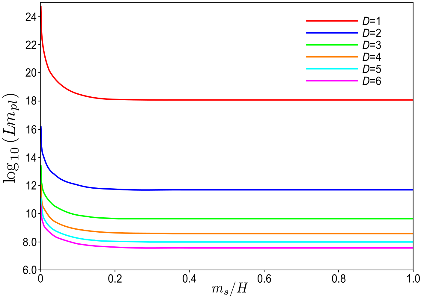
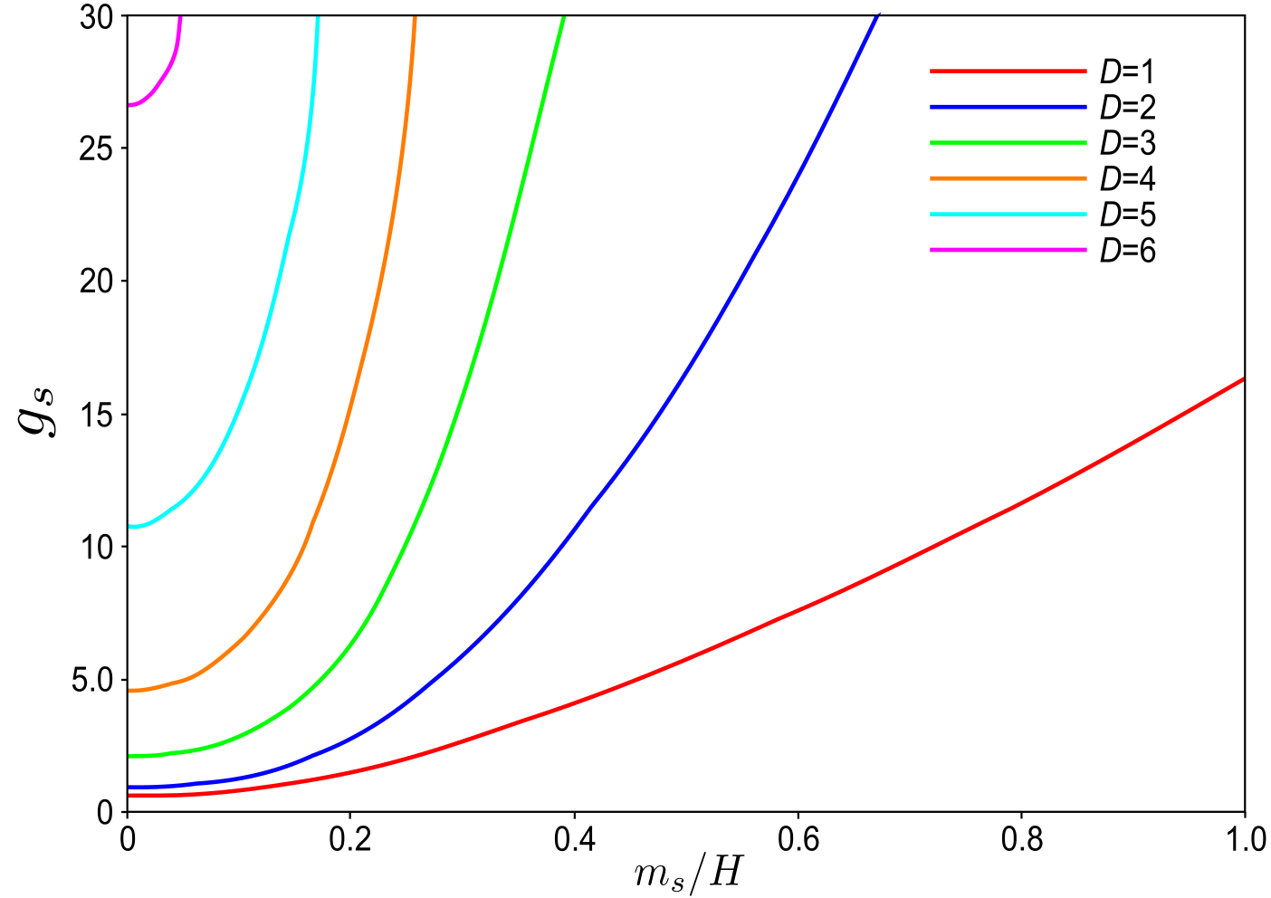
Figs. 3 and 4 show and as functions of , respectively. It is easier to have weak coupling with small , while it is easier to keep not too large with large . Typical values that are consistent with (5.6) would be:
| (5.7) | ||||
| (5.8) | ||||
| (5.9) |
The number of the fields that participate in is roughly . For the above choice of parameters, .
6 Time-dependent Hubble
So far we have studied the fluctuations generated during inflation, assuming the background is pure de Sitter. Let us now consider the effect of time-dependent Hubble.
6.1 Spectral index
Since originates from the fluctuations of massive fields, the spectrum is stronger in the UV. The spectral index is slightly larger than 1,
| (6.1) | |||||
This is in the range when , and for (See Figure 5).

The above values are obtained by assuming the Hubble is constant. However, is sensitive to the time-dependence of . As long as the change of Hubble is adiabatic , it would be reasonable to assume the amplitudes are determined in terms of at the time of horizon crossing. We will have to replace the prefactor in the two-point function (4.12) to where is the time of the horizon exit for the scale of interest (). Since the long wave length mode exits the horizon early, the amplitude is lifted in the infrared. The spectral index is lowered by if there is time-dependence of order .
It would be necessary to understand the origin of vacuum energy during inflation to understand its time-dependence. In this paper, we cannot make a definitive statement, but we would like to mention a possible origin of vacuum energy in the next subsection.
6.2 Possible origin of vacuum energy
In most inflationary models, the presence of vacuum energy (or a nearly flat inflaton potential) is simply assumed and its origin is not clear. Also, in the recent constructions of de Sitter vacua in string theory, the mechanism for uplifting from supersymmetric vacua to de Sitter vacua is not fully understood. In the study of low energy effective action of string theory, it has been very difficult to find de Sitter vacua in a controllable approximation. (See e.g. [22] for a recent discussion.)
It might be necessary to understand vacuum fluctuations of the fields to find de Sitter vacua. In string compactification models with large internal space [23], which is believed to be realizable generically, there are many light KK fields. Quantum fluctuations of these fields might be an important source of vacuum energy.
With this motivation in mind, in this subsection, we discuss a possible dynamical scenario in which vacuum fluctuations and Hubble are determined in a self-consistent manner.
Consider the expectation value (one-point function) of the energy-momentum tensor. This quantity is UV divergent, and we will renormalize it so that it vanishes in the flat background. Because of de Sitter symmetry, the expectation value is proportional to .
The renormalized expectation value of energy-momentum tensor of a scalar field in de Sitter background is given by (see (6.183) of [21])
| (6.2) |
where , and is the order of Hankel function as described in Section 2. is renormalized by subtracting the divergent piece in the flat background. When there are scalar fields (assuming massless minimally coupled), we have
| (6.3) |
It would be possible that de Sitter space during inflation is a self-consistent solution of
| (6.4) |
The condition that both sides of the equation balances implies
| (6.5) |
In fact, our scenario is not consistent with this equation as it is. The value of which produces the observed level of temperature fluctuations is at least with , and is too large by a factor of for (6.4) to be satisfied. However, this is not a contradiction. We do not expect that Einstein equation (6.4) is applicable, since our preferred value of string coupling is , and the left hand side will be corrected by string () effects, which are not negligible when .
Presumably, the self-consistent de Sitter solution of (6.4) is an unstable solution, and small fluctuation of will drive the background to flat space, which is another solution of this equation. To study time-dependence, we will have to compute the expectation value in the background with . This with (6.4) will tell us the evolution of Hubble. We will leave this analysis as an important open question.
It is not clear whether the dynamics of quantum expectation value is similar to the dynamics of inflaton, but let us assume it is for the moment. In Appendix A, we perform the analysis of fluctuations including inflaton fluctuations . We take to be of the same order as , . The gravitational potential has a term induced by in addition to the term from the matter fields that we have studied. The relative importance of inflaton and the matter fields depends on the details, such as the slope of the inflaton potential and the time between horizon crossing and the end of inflation. The effect of the matter fields will be important unless the slope is fine tuned to a small value.
7 Non-gaussianities
Non-gaussianities appear in a characteristic manner in our mechanism. We first describe the calculation ignoring interactions among the matter fields . We then remark that the magnitude of non-gaussianities is controlled by the coupling constant in higher dimension.
The three-point function of is given by the triangle diagram where each pair of points is connected by (see Figure 7),
| (7.1) | |||
We define the non-linearity parameter by a local replacement, [24], with a gaussian field . Let us consider three-points at superhorizon separation, and estimate by expansing the coordinates as in (5.3). The local form of is enough to characterize the magnitude of non-gaussianity in this approximation. From (7.1),
| (7.2) |
This is proportional to , and further suppressed by the other factors (See Fig 6). For , we have

The reason for the smallness of non-gaussianity is that is roughly proportional to the number of fields , and is also proportional to in our setting. This makes the non-gaussianity small in the large limit. This is in contrast to the curvaton case [16], where non-gaussianity is necessarily large if curvaton is the only source of curvature fluctuations [18].

When there are interactions among ’s, we will have higher loop diagrams, such as the ones in which a propagator traverses two sides of the triangle. (See Figure 7.) Even though there are many fields, interactions do not necessarily make huge. Since the fields are KK modes or string states, there will be conserved quantities such as momentum in the internal space or the excitation number of strings. The third field in the right diagram in Figure 7 is determined by the first two, and this diagram will be of order . The natural magnitude of the coupling will be where is the coupling constant in higher dimension, and is the volume of internal space. This is because the canonically normalized KK fields has a factor relative to the higher dimensional field, and the interaction has one more than the kinetic term. Since as mentioned in Section 4.1, the factor associated to the right diagram of Figure 7 is just given by . (This is equivalent to saying that the correlation functions are computed by Feynman rules in the higher dimensions with the diagrams of the type of Figure 7.)
If takes finite but small enough value that perturbation theory is applicable, non-gaussianities will be given by the diagrams such as the ones in Figure 7. The shape (momentum dependence) [25] of this type of non-gaussianity will be different from those arising from the usual slow-roll inflation [26]. The difference will be seen by studying the three-point correlations at subhorizon separations. We will leave this analysis to future study.
8 Conclusions
We have shown that the CMB temperature fluctuations (adiabatic perturbation) can be generated by the purely quantum effects of fields which are classically at rest. When there are a large number of fields, this can produce observable level of fluctuations. Tensor fluctuations are hardly affect by this effect, and will remain of order . In our mechanism, the enhancement of scalar fluctuations relative to tensor fluctuation is due to the large number of fields involved, and not due to the smallness of the slow-roll parameter as in the usual slow-roll scenario.
When the size of the extra dimensions are large compared to the inverse Hubble during inflation, we have a large number of Kaluza-Klein modes which contribute to this effect. String excited modes also contribute if . We compare our results with observed amplitude, and find that is preferred. The size of extra dimensions is typically of order GeV-1 or smaller.
There have been models of inflation based on TeV scale supersymmetry (see [28] for a review). Inflation and reheating have been studied in explicit string compactification in [27]: Supersymmetry is broken by the hidden-sector branes wrapped around internal cycles, and inflaton is given by closed string moduli. In that case, it is important to make sure that the decay of inflaton reheats the visible sector dominantly and not the hidden sectors significantly, which has been checked in [27]. This is necessary to avoid cosmological problems, such as the generation of large isocurvature perturbations.
In our case, we do not assume low-energy supersymmetry. In this case, it will be generically the case that massive fields, such as KK modes, decay and reach thermal equilibrium. This will occur well before the standard big bang nucleosynthesis begins. In this situation, there will be no isocurvature perturbations, as shown in [19].
We performed our analysis assuming the extra dimensions are compactified on a torus . We believe this captures the qualitative features of quantum effects of KK states in the general compactifications with , whenever the multiplicity of the KK modes is similar to that for . There have been studies on string compactifications which realizes supersymmetric vacua with all moduli fixed. It is argued that the large-volume compactification is generically achievable in the construction of [23]. Understanding of the mechanism for uplifting to de Sitter vacua or realizing inflation is at a more qualitative level at present. Brane anti-brane pair [29] will be a candidate for such a mechanism. We expect our mechanism for generating CMB temperature fluctuations should be relevant in these contexts.
Non-gaussianity in our mechanism is given by triangle diagrams, with possible corrections. The magnitude is controlled by the coupling constant in higher dimension. It would be possible in principle to distinguish our mechanism from others by the precise measurement of non-gaussianities.
The main purpose of this paper is to study fluctuations without asking the origin of vacuum energy during inflation. But as we mentioned in Section 6, it would be possible that vacuum fluctuations (the renormalized expectation value of energy-momentum tensor) of a large number of fields are the source of vacuum energy. It is important to understand the dynamics of this vacuum energy [30]. We have included the analysis of fluctuations in the background with time-dependent Hubble by introducing inflaton in the appendix, but it is not clear to what extent this captures the dynamics of quantum vacuum energy.
Acknowledgements
We thank Misao Sasaki for helpful comments. The work of H.K is supported by the MEXT Grant-in-Aid for the Global COE Program, “The Next Generation of Physics Spun from Universality and Emergence,” and the JSPS Grant-in-Aid for Scientific Research No. 22540277. M.N is supported by the JSPS Grant-in-Aid for Scientific Research Nos. 21540290 and 23540332. Y.S is supported by JSPS Grant-in-Aid for Scientific Research (A) No. 23244057, and the MEXT Grant-in-Aid for Young Scientists (B) No. 21740216. M.N acknowledges the Niels Bohr Institute for their hospitality extended during his stay.
Appendix
Appendix A Perturbations including inflaton
In this appendix, we assume the dynamics of time-dependent Hubble is effectively described by an inflaton field , and study fluctuations including the inflaton fluctuation in addition to matter fields .
We assume inflaton and matter are not directly coupled with each other. Thus, the equation of motion for is the same as before, except that Hubble is now time-dependent and and are not those for pure de Sitter,
| (A.1) |
This does not couple to fluctuations of other fields, so the quantization of can be done at first.
The action of inflaton is
| (A.2) |
We decompose into classical part (which is homogeneous in space) and fluctuations,
| (A.3) |
Classical part satisfies the equation of motion
| (A.4) |
To find the equation of motion for , it is convenient to take the longitudinal gauge,
| (A.5) |
and expand the equation of motion,
| (A.6) |
to the first order in , , . Then, we get
| (A.7) |
Energy-momentum tensor for is
| (A.8) |
The classical part (zeroth order in ) is
| (A.9) | |||||
| (A.10) |
The linear part in is
| (A.11) | |||||
| (A.12) | |||||
| (A.13) |
Note that does not have off-diagonal components.
To write Einstein equations, we include the linear terms in and the quadratic terms in in the energy-momentum tensor. The (0,0), (0, ) and (, ) components of Einstein equations are as follows:
| (A.14) | |||
| (A.15) | |||
| (A.16) |
where the summation is taken over the species of matter fields , as in the main text.
Let us study the leading behavior in the super-horizon limit following [1]. We assume inflaton is classically slow-rolling,
| (A.17) |
We consider inflaton e.o.m. (A.7) and the (0, ) component of Einstein equation (A.15). In terms of physical time (and in the slow-roll limit),
| (A.18) | |||
| (A.19) |
where we have ignored the terms in the energy momentum tensor of which are small in the small mass limit, (we ignore the term in (3.14)).
These equations imply
| (A.20) |
where we have defined by
| (A.21) |
That is,
| (A.22) |
in the late time limit. From (A.20),
| (A.23) |
with a constant . We fix so that the amplitude of is at the horizon exit (since is essentially a massless scalar inside the horizon),
| (A.24) |
where the star denotes the quantities evaluated at the horizon exit.
In the usual slow-roll inflation, there is only the first term. The factor generally grows towards the end of inflation, and it is assumed to be of order at the end of inflation. The second term represents the effect of matter fields to the evolution of inflaton fluctuation.
In terms of ,
| (A.25) | |||||
| (A.26) |
The first term is the part induced from the inflaton fluctuation (A.24) through the usual mechanism. The second term is the effect of matter (agrees with the formula that we have obtained), which exists even if there is no inflaton.
This expression will be valid until the end of inflation. After inflation, will be constant (assuming is classically oscillating, in which case it can be regarded as matter, or has decayed into radiation). Relative importance of the effect of compared to that of inflaton in (A.26) depends on the details such as how steep the potential is or how much time has passed between horizon exit and the end of inflation.
References
- [1] V. Mukhanov, “Physical Principles of Cosmology,” Cambridge University Press, Cambridge, 2005.
- [2] A. H. Guth, “The Inflationary Universe: A Possible Solution to the Horizon and Flatness Problems,” Phys. Rev. D23, 347-356 (1981).
- [3] A. D. Linde, “Particle physics and inflationary cosmology,” Harwood, Chur, Switzerland, 1990. (Contemporary concepts in physics, 5) [hep-th/0503203].
- [4] E. Komatsu et al. [WMAP Collaboration], “Seven-Year Wilkinson Microwave Anisotropy Probe (WMAP) Observations: Cosmological Interpretation,” Astrophys. J. Suppl. 192, 18 (2011).
- [5] S. W. Hawking, “The Development of Irregularities in a Single Bubble Inflationary Universe,” Phys. Lett. B115, 295 (1982); A. A. Starobinsky, “Dynamics of Phase Transition in the New Inflationary Universe Scenario and Generation of Perturbations,” Phys. Lett. B117, 175-178 (1982); A. H. Guth, S. Y. Pi, “Fluctuations in the New Inflationary Universe,” Phys. Rev. Lett. 49, 1110-1113 (1982); J. M. Bardeen, P. J. Steinhardt, M. S. Turner, “Spontaneous Creation of Almost Scale - Free Density Perturbations in an Inflationary Universe,” Phys. Rev. D28, 679 (1983).
- [6] A. D. Linde, “A New Inflationary Universe Scenario: A Possible Solution of the Horizon, Flatness, Homogeneity, Isotropy and Primordial Monopole Problems,” Phys. Lett. B108, 389-393 (1982); A. Albrecht, P. J. Steinhardt, “Cosmology for Grand Unified Theories with Radiatively Induced Symmetry Breaking,” Phys. Rev. Lett. 48, 1220-1223 (1982).
- [7] A. D. Linde, “Chaotic Inflation,” Phys. Lett. B129, 177-181 (1983).
- [8] S. Dimopoulos, S. Kachru, J. McGreevy and J. G. Wacker, “N-flation,” JCAP 0808, 003 (2008); A. R. Liddle, A. Mazumdar and F. E. Schunck, “Assisted inflation,” Phys. Rev. D 58, 061301 (1998).
- [9] V. F. Mukhanov, “Gravitational Instability of the Universe Filled with a Scalar Field,” JETP Lett. 41, 493-496 (1985); “Quantum Theory of Gauge Invariant Cosmological Perturbations,” Sov. Phys. JETP 67, 1297-1302 (1988); M. Sasaki, “Large Scale Quantum Fluctuations in the Inflationary Universe,” Prog. Theor. Phys. 76, 1036 (1986).
- [10] S. M. Leach, M. Sasaki, D. Wands, A. R. Liddle, “Enhancement of superhorizon scale inflationary curvature perturbations,” Phys. Rev. D 64, 023512 (2001).
- [11] D. H. Lyth, A. R. Liddle, “The primordial density perturbation: Cosmology, inflation and the origin of structure,” Cambridge University Press, Cambridge, 2009.
- [12] A. A. Starobinsky, “Relict Gravitation Radiation Spectrum and Initial State of the Universe,” JETP Lett. 30, 682-685 (1979).
- [13] Y. Nambu, M. Sasaki, “Purely Quantum Derivation Of Density Fluctuations In The Inflationary Universe,” Prog. Theor. Phys. 83, 37 (1990).
- [14] Y. Habara, H. Kawai, M. Ninomiya, Y. Sekino, “CMB Fluctuations and String Compactification Scales,” Phys. Lett. B 707, 198 (2012).
- [15] M. Spradlin, A. Strominger, A. Volovich, “Les Houches lectures on de Sitter space,” [hep-th/0110007].
- [16] D. H. Lyth and D. Wands, “Generating the curvature perturbation without an inflaton,” Phys. Lett. B 524, 5 (2002); K. Enqvist and M. S. Sloth, “Adiabatic CMB perturbations in pre - big bang string cosmology,” Nucl. Phys. B 626, 395 (2002); T. Moroi, T. Takahashi, “Effects of cosmological moduli fields on cosmic microwave background,” Phys. Lett. B522, 215-221 (2001).
- [17] E. Komatsu et al. [WMAP Collaboration], “Five-Year Wilkinson Microwave Anisotropy Probe (WMAP) Observations: Cosmological Interpretation,” Astrophys. J. Suppl. 180, 330 (2009).
- [18] D. H. Lyth, C. Ungarelli and D. Wands, “The Primordial density perturbation in the curvaton scenario,” Phys. Rev. D 67, 023503 (2003).
- [19] S. Weinberg, “Must cosmological perturbations remain non-adiabatic after multi-field inflation?,” Phys. Rev. D 70, 083522 (2004).
- [20] A. Golovnev, V. Mukhanov and V. Vanchurin, “Vector Inflation,” JCAP 0806, 009 (2008).
- [21] N. D. Birrell, P. C. W. Davies, “Quantum Fields In Curved Space,” Cambridge University Press, Cambridge, 1982.
- [22] X. Chen, G. Shiu, Y. Sumitomo and S. H. H. Tye, “A Global View on The Search for de-Sitter Vacua in (type IIA) String Theory,” arXiv:1112.3338 [hep-th].
- [23] V. Balasubramanian, P. Berglund, J. P. Conlon, F. Quevedo, “Systematics of moduli stabilisation in Calabi-Yau flux compactifications,” JHEP 0503, 007 (2005). J. P. Conlon, F. Quevedo, K. Suruliz, “Large-volume flux compactifications: Moduli spectrum and D3/D7 soft supersymmetry breaking,” JHEP 0508, 007 (2005).
- [24] E. Komatsu and D. N. Spergel, “Acoustic signatures in the primary microwave background bispectrum,” Phys. Rev. D 63, 063002 (2001).
- [25] D. Babich, P. Creminelli and M. Zaldarriaga, “The Shape of non-Gaussianities,” JCAP 0408, 009 (2004); L. Senatore, K. M. Smith and M. Zaldarriaga, “Non-Gaussianities in Single Field Inflation and their Optimal Limits from the WMAP 5-year Data,” JCAP 1001, 028 (2010).
- [26] J. M. Maldacena, “Non-Gaussian features of primordial fluctuations in single field inflationary models,” JHEP 0305, 013 (2003); N. Bartolo, E. Komatsu, S. Matarrese, A. Riotto, “Non-Gaussianity from inflation: Theory and observations,” Phys. Rept. 402, 103-266 (2004).
- [27] M. Cicoli and A. Mazumdar, “Reheating for Closed String Inflation,” JCAP 1009, 025 (2010); M. Cicoli and A. Mazumdar, “Inflation in string theory: A Graceful exit to the real world,” Phys. Rev. D 83, 063527 (2011).
- [28] A. Mazumdar and J. Rocher, “Particle physics models of inflation and curvaton scenarios,” Phys. Rept. 497, 85 (2011).
- [29] G. R. Dvali, S. H. H. Tye, “Brane inflation,” Phys. Lett. B450, 72-82 (1999).
- [30] Y. Habara, H. Kawai, M. Ninomiya, Y. Sekino, work in progress.