Geometry of the 3-user MIMO
interference channelThanks: This paper appeared in the Allerton conference on communication, control, and computing held September 28-30, 2011

Before providing rigorous arguments, in this subsection we describe the geometry underlying the problem. Relevant definitions are provided in subsequent sections.

A given vector $u_{i}$ in the signal space of transmitter $i$ is said to initiate an alignment path of length $r+1$ if there exists a sequence of vectors $u_{i+1},u_{i+2},\dots,u_{i+r}\in{\mathbb{C}}^{M}$, such that $\mathbf{H}^{[i-1,i]}u_{i}=\mathbf{H}^{[i-1,i+1]}u_{i+1},\dots,\mathbf{H}^{[i+r-2,i+r-1]}u_{i+r-1}=\mathbf{H}^{[i+r-2,i+r]}u_{i+r}$. Here channel indices are interpreted modulo 3. For example, a vector $u_{2}$ at transmitter 2 initiating an alignment path of length 3 means that there exist vectors $u_{3}$ and $u_{1}$ such that $\mathbf{H}^{[12]}u_{2}=\mathbf{H}^{[13]}u_{3}$ and $\mathbf{H}^{[23]}u_{3}=\mathbf{H}^{[21]}u_{1}$.

The feasible region of Figure 1 is divided up into sub-regions labeled with the maximum length of an alignment path; this number depends on $M$ and $N$ through the incidence geometry of the images of the channel matrices $\mathrm{Im}(\mathbf{H}^{[ij]})$. We begin by examining sub-region 1, and then look at how things generalize to the other sub-regions.

The point of departure is the obvious constraint $d\leq M$ in order to have a $d$-dimensional subspace of an $M$ dimensional vector space. Continuing, assuming $M\geq d$, suppose $2M\leq N$, so $(M,N)$ lies in sub-region 1 of Figure 1. At receiver one, the images $\mathrm{Im}(\mathbf{H}^{[12]})$ and $\mathrm{Im}(\mathbf{H}^{[13]})$ of the channels from transmitters two and three are in general position and therefore their intersection has dimension $[2M-N]^{+}=0$; in other words, alignment is impossible in sub-region 1. Figure 2 shows pictorially that because alignment is not possible here, we have the constraint $3d\leq N$. Mathematically, we see that alignment is not possible because the map from ${\mathbb{C}}^{2M}$ to ${\mathbb{C}}^{N}$ given by the matrix $\left(\begin{matrix}\mathbf{H}^{[12]}&\mathbf{H}^{[13]}\end{matrix}\right)$ is injective.

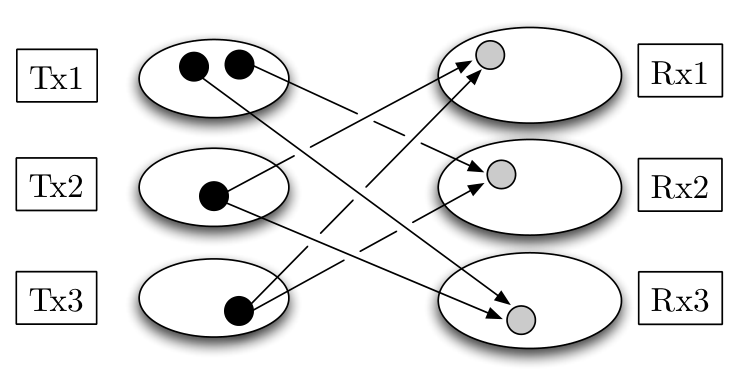
Moving onward to sub-region 2, we have $2M>N$ and thus alignment is possible. This means that alignment paths of length 2 are possible (Fig 3), with up to $2M-N$ interference dimensions overlapping at each receiver. Thus, the interference space $\mathbf{H}^{[12]}U_{2}+\mathbf{H}^{[13]}U_{3}$ at receiver one occupies at least $2d-(2M-N)$ dimensions, and we have the constraint $3d\leq 2M$. However, because $3M\leq 2N$, no vector at (say) transmitter three can be simultaneously aligned at both receivers one and two, as indicated in Figure 4. One can also see that no simultaneous alignment is possible by changing change perspective to that of a combined receiver one and two. One may check directly that (as a special case of Lemma 2), the map

from the three transmitters to ${\mathbb{C}}^{2N}$ is injective; analogously to the case in sub-region 1, this is interpreted to mean that no alignment is possible in the combined receive space ${\mathbb{C}}^{2N}$ (see Fig. 5). Thus, five complementary $d$-dimensional subspaces lie in ${\mathbb{C}}^{2N}$ and we obtain the constraint $5d\leq 2N$.

As far as achievability goes, the basic rule-of-thumb is to create alignment paths of maximum length. Thus, in sub-region 2, where alignment is possible, the achievable strategy aligns as many vectors as possible and the remaining ones (if $d>2(2M-N)$) are not aligned.

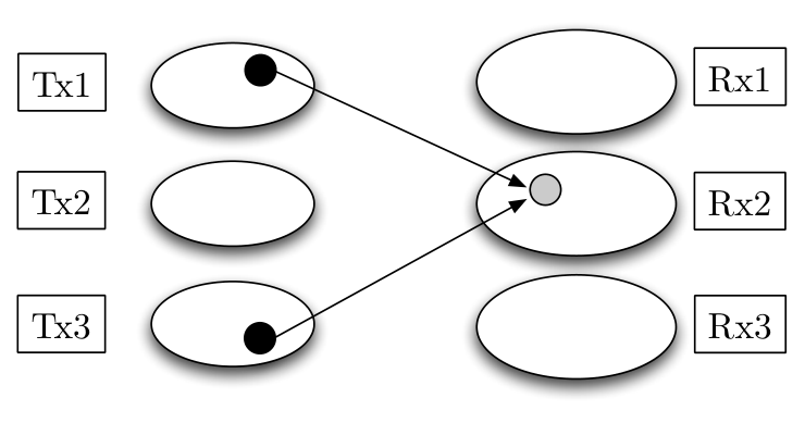
Both the necessary conditions and achievability arguments extend in a natural way. On the achievability end, alignment paths of maximum length are used. For example, in sub-region 4, alignment paths of length four are used (Fig 6). For the converse, a generalization of the matrix in (2) is shown to be full-rank in Lemma 2, giving the constraints in (1).

The problem we consider, of maximizing degrees-of-freedom using linear strategies for the $K$-user MIMO IC with finite number of transmit and receive antennas, has received significant attention in the last several years. Jafar and Fakhereddin [4] determined the degrees of freedom of the two-user MIMO IC with an arbitrary number of antennas at each of the four terminals. Cadambe and Jafar [3] considered the problem for $K=3$ users and $N=2$ antennas, and showed that $3/2$ dof was achievable. For more than $3$ users or $N>2$ they assumed infinite time or frequency diversity and applied their main $K/2$ result. Gomadam et al. [5, 6], posed the problem of determining feasibility of linear alignment in the constant channel setting, but left the problem unanswered and proposed a heuristic iterative numerical algorithm.

Also at the heuristic level, Yetis et al. [7] proposed to determine feasibility of alignment by counting the number of equations and comparing to the number of variables. This approach was carried out rigorously to show a necessary and sufficient condition in [8] for the symmetric square case of $N=M$ antennas at all $K$ transmitters and receivers and by Razaviyayn et al. [9] for the case that the number of transmit dimensions $d$ divides both the number of transmit and receive antennas. Several other works have subsequently pursued a similar approach for related problems, including [10], [11] (both heuristic), and [12].

The remaining work on linear alignment for the MIMO IC has focused on heuristic algorithms, mainly iterative in nature (see [6], [13], [14], [15], and [16]). Some have proofs of convergence, but no performance guarantees are known.

We emphasize that in this paper we restrict attention to vector space interference alignment, where the effect of finite channel diversity can be observed. Interfering signals can also be aligned on the signal scale using lattice codes (first proposed in [17], see also [18], [19], [20]), however the understanding of this type of alignment is currently at the stage corresponding to infinite time or frequency diversity in the vector space setting. In other words, essentially “perfect” alignment is possible due to the infinite channel precision available at infinite signal-to-noise ratios.

Ghasemi et al. [21] apply alignment on the signal scale to the $K$-user $M\times N$ MIMO IC. The converse arguments in that paper are obtained by forming a two-user interference channel with two users transmitting and decoding jointly; thus they obtain the inequality $3d\leq\max(N,2M)$ corresponding to $r=1$ in (1) of the present paper.

In exactly the same setting as the present paper, Amir et al. [22] have independently proposed a similar achievable strategy for critical $M,N$ satisfying both (1) and $M+N=4d$. [22] is limited to critical values of $M,N$ and contains no converse arguments beyond the equation counting bound of [8] and [9].

Finally, also independently, Wang et al. [23] very recently posted a paper to the Arxiv containing many similar results. Their converse is information theoretic and, unlike ours, is not limited to linear strategies.

The $K$-user MIMO interference channel has $K$ transmitters and $K$ receivers, with transmitter $i$ having $M_{i}$ antennas and receiver $i$ having $N_{i}$ antennas. For $i=1,\dots,K$, receiver $i$ wishes to obtain a message from the corresponding transmitter $i$. The remaining signals from transmitters $j\neq i$ are undesired interference. The channel is assumed to be constant over time, and at each time-step the input-output relationship is given by

Here for each user $i$ we have $\mathbf{x}_{i}\in{\mathbb{C}}^{M_{i}}$ and $\mathbf{y}_{i},\mathbf{z}_{i}\in{\mathbb{C}}^{N_{i}}$, with $\mathbf{x}_{i}$ the transmitted signal, $\mathbf{y}_{i}$ the received signal, and $\mathbf{z}_{i}\sim\mathcal{CN}(0,I_{N_{i}})$ is additive isotropic white Gaussian noise. The channel matrices are given by $\mathbf{H}^{[ij]}\in{\mathbb{C}}^{N_{i}\times M_{j}}$ for $1\leq i,j\leq K$, with each entry assumed to be independent and with a continuous distribution. We note that this last assumption on independence can be weakened significantly to a basic non-degeneracy condition but we will not pursue this here. For our purposes this means the channel matrices are generic. Each user has an average power constraint, $E(||\mathbf{x}_{i}||^{2})\leq P$.

We restrict the class of coding strategies to (linear) vector space strategies. In this context degrees-of-freedom (dof) has a simple interpretation as the dimensions of the transmit subspaces, described in the next paragraph. However, note that one can more generally define the degrees-of-freedom region in terms of an appropriate high transmit-power limit $P\to\infty$ of the Shannon capacity region $C(P)$ normalized by $\log P$ ([3], [2]). In that general framework, it is well-known and easy to show that vector space strategies give a concrete non-optimal achievable strategy with rates

Here $d_{i}$ is the dimension of transmitter $i$’s subspace and $P$ is the transmit power.

The transmitters encode their data using vector space precoding. Suppose transmitter $j$ wishes to transmit a vector $\hat{x}_{j}\in\mathbb{C}^{d_{j}}$ of $d_{j}$ data symbols. These data symbols are modulated on the subspace $U_{j}\subseteq{\mathbb{C}}^{M_{j}}$ of dimension $d_{j}$, giving the input signal $\mathbf{x}_{j}=\mathbf{U}_{j}\hat{x}_{j}$, where $\mathbf{U}_{j}$ is a $M_{j}\times d_{j}$ matrix whose column span is $U_{j}$. The signal $\mathbf{x}_{j}$ is received by receiver $i$ through the channel as $\mathbf{H}^{[ij]}\mathbf{U}_{j}\hat{x}_{j}$ The dimension of the transmit space, $d_{j}$, determines the number of data streams, or degrees-of-freedom, available to transmitter $j$. With this restriction of strategies, the output is given by

The desired signal space at receiver $i$ is thus $\mathbf{H}^{[ii]}U_{i}$, while the interference space is given by $\sum_{j\neq i}\mathbf{H}^{[ij]}U_{j}$, i.e. the span of the undesired subspaces as observed by receiver $i$.

In the regime of asymptotically high transmit powers, in order that decoding can be accomplished we impose the constraint at each receiver $i$ that the desired signal space $\mathbf{H}^{[ii]}U_{i}$ is complementary to the interference space $\sum_{j\neq i}\mathbf{H}^{[ij]}U_{j}$. Equivalently, there must exist subspaces $V_{i}$ with $\dim V_{i}=\dim U_{i}$ such that

and

Here $\mathbf{H}^{[ij]}U_{j}\perp V_{i}$ is interpreted to mean that $V_{i}$ belongs to the dual space $({\mathbb{C}}^{N_{i}})^{*}$ and $V_{i}$ annihilates $\mathbf{H}^{[ij]}U_{j}$. Alternatively, $(\mathbf{V}_{i})^{\dagger}\mathbf{H}^{[ij]}\mathbf{U}_{j}=0$, where $\mathbf{V}^{\dagger}$ denotes the Hermitian transpose of $\mathbf{V}$ and $\mathbf{V}_{i}$ is a matrix with column span equal to $V_{i}$. Note that implicitly the transmit dimensions are assumed to satisfy the obvious inequality $d_{i}\leq\min(M_{i},N_{i})$. If each direct channel matrix $\mathbf{H}^{[ii]}$ has generic (or i.i.d. continuously distributed) entries, then the second condition (6) is satisfied assuming $\dim V_{i}=d_{i}$ for each $i$ (this can be easily justified—see [5] for some brief remarks). Hence we focus on condition (5).

The goal is to maximize degrees of freedom, i.e. choose subspaces $U_{1},\dots,U_{K}$, $V_{1},\dots,V_{K}$ with $d_{i}\leq\min(M_{i},N_{i})$ in order to

To this end, it is sufficient to answer the following feasibility question: given number of users $K$, number of antennas $M_{1},\dots,M_{K}$, $N_{1},\dots,N_{K}$, and desired transmit subspace dimensions $d_{1},\dots,d_{K}$, does there exist a choice of subspaces $U_{1},\dots,U_{K}$ and $V_{1},\dots,V_{K}$ with $\dim U_{i}=\dim V_{i}=d_{i},1\leq i\leq K$, satisfying (5)?

For the rest of the paper, we fix $K=3$, and we introduce two notational conveniences for this case. First, we interpret the indices modulo three, so that $\mathbf{H}^{[12]}=\mathbf{H}^{[42]}$ and so on. Second, since the indices can always be chosen to differ by exactly one, we will adopt the shorthand $\mathbf{H}^{[i,+]}$ and $\mathbf{H}^{[i,-]}$ for $\mathbf{H}^{[i,i+1]}$ and $\mathbf{H}^{[i,i-1]}$ respectively.

References

- [1] G. Bresler and D. Tse, “Degrees-of-freedom for the 3-user Gaussian interference channel as a function of channel diversity,” in Allerton Conference on Communication, Control, and Computing, September 2009.
- [2] M. Maddah-Ali, A. Motahari, and A. Khandani, “Communication over MIMO X channels: Interference alignment, decomposition, and performance analysis,” IEEE Trans. Inf. Theory, vol. 54, pp. 3457 –3470, August 2008.
- [3] V. Cadambe and S. Jafar, “Interference alignment and degrees of freedom of the -user interference channel,” IEEE Trans. Inf. Theory, vol. 54, pp. 3425 –3441, August 2008.
- [4] S. Jafar and M. Fakhereddin, “Degrees of freedom for the MIMO interference channel,” IEEE Trans. Inf. Theory, vol. 53, pp. 2637 –2642, July 2007.
- [5] K. Gomadam, V. Cadambe, and S. Jafar, “Approaching the capacity of wireless networks through distributed interference alignment,” in IEEE GLOBECOM, pp. 1 –6, December 2008.
- [6] K. Gomadam, V. Cadambe, and S. Jafar, “A distributed numerical approach to interference alignment and applications to wireless interference networks,” Information Theory, IEEE Transactions on, vol. 57, pp. 3309 –3322, June 2011.
- [7] C. Yetis, T. Gou, S. Jafar, and A. Kayran, “On feasibility of interference alignment in MIMO interference networks,” IEEE Trans. Signal Processing, vol. 58, pp. 4771 –4782, September 2010.
- [8] G. Bresler, D. Cartwright, and D. Tse, “Settling the feasibility of interference alignment for the MIMO interference channel: the symmetric square case,” April 2011. arXiv:1104.0888v1.
- [9] M. Razaviyayn, L. Gennady, and Z. Luo, “On the degrees of freedom achievable through interference alignment in a MIMO interference channel.” arXiv:1104.0992v1.
- [10] B. Zhuang, R. Berry, and M. Honig, “Interference alignment in MIMO cellular networks,” in ICASSP 2011, pp. 3356–3359, May 2011.
- [11] M. Guillaud and D. Gesbert, “Interference alignment in the partially connected K-user MIMO interference channel,” in European Signal Processing Conference (EUSIPCO), August 2011.
- [12] V. S. Annapureddy, A. El Gamal, and V. V. Veeravalli, “Degrees of freedom of interference channels with CoMP transmission and reception,” September 2011. arXiv:1109.5396v1.
- [13] S. Peters and R. Heath, “Interference alignment via alternating minimization,” in Acoustics, Speech and Signal Processing, 2009. IEEE International Conference on, pp. 2445 –2448, April 2009.
- [14] M. Razaviyayn, M. Sanjabi Boroujeni, and Z.-Q. Luo, “Linear transceiver design for interference alignment: Complexity and computation,” in Signal Processing Advances in Wireless Communications (SPAWC), 2010 IEEE Eleventh International Workshop on, pp. 1 –5, June 2010.
- [15] D. S. Papailiopoulos and A. G. Dimakis, “Interference alignment as a rank constrained rank minimization,” in IEEE GLOBECOM, 2010.
- [16] I. Santamaria, O. Gonzalez, R. Heath, and S. Peters, “Maximum sum-rate interference alignment algorithms for MIMO channels,” in IEEE GLOBECOM, pp. 1 –6, December 2010.
- [17] G. Bresler, A. Parekh, and D. Tse, “The approximate capacity of the many-to-one and one-to-many Gaussian interference channels,” IEEE Trans. Inf. Theory, vol. 56, September 2010.
- [18] V. Cadambe, S. Jafar, and S. Shamai, “Interference alignment on the deterministic channel and application to fully connected gaussian interference networks,” IEEE Trans. Inf. Theory, vol. 55, pp. 269 –274, January 2009.
- [19] R. Etkin and E. Ordentlich, “The degrees-of-freedom of the -user gaussian interference channel is discontinuous at rational channel coefficients,” IEEE Trans. Inf. Theory, vol. 55, pp. 4932 –4946, November 2009.
- [20] A. S. Motahari, S. Gharan, M. Maddah-Ali, and A. K. Khandani, “Real interference alignment: Exploiting the potential of single antenna systems,” August 2009. arXiv:0908.2282v2.
- [21] A. Ghasemi, A. Motahari, and A. Khandani, “Interference alignment for the K user MIMO interference channel,” in Information Theory Proceedings (ISIT), 2010 IEEE International Symposium on, pp. 360 –364, June 2010.
- [22] M. Amir, A. El-Keyi, and M. Nafie, “A new achievable DoF region for the 3-user symmetric interference channel,” May 2011. arXiv:1105.4026v1.
- [23] C. Wang, T. Gou, and S. Jafar, “Subspace alignment chains and the degrees of freedom of the three-user MIMO interference channel,” September 2011. arXiv:1109.4350v1.
- [24] R. Hartshorne, Algebraic Geometry. Graduate Texts in Mathematics, Springer, 1st ed., 1977.