Wavemoth – Fast spherical harmonic transforms by butterfly matrix compression
Abstract
We present Wavemoth, an experimental open source code for computing scalar spherical harmonic transforms (SHTs). Such transforms are ubiquitous in astronomical data analysis. Our code performs substantially better than existing publicly available codes due to improvements on two fronts. First, the computational core is made more efficient by using small amounts of precomputed data, as well as paying attention to CPU instruction pipelining and cache usage. Second, Wavemoth makes use of a fast and numerically stable algorithm based on compressing a set of linear operators in a precomputation step. The resulting SHT scales as for the resolution range of practical interest, where denotes the spherical harmonic truncation degree. For low and medium-range resolutions, Wavemoth tends to be twice as fast as libpsht, which is the current state of the art implementation for the HEALPix grid. At the resolution of the Planck experiment, , Wavemoth is between three and six times faster than libpsht, depending on the computer architecture and the required precision. Due to the experimental nature of the project, only spherical harmonic synthesis is currently supported, although adding support for spherical harmonic analysis should be trivial.
Subject headings
Methods: numericalI. Background
The spherical harmonic transform (SHT) is the spherical analog of the Fourier transform, and is an essential tool for data analysis and simulation on the sphere. A scalar field on the unit sphere can be expressed as a weighted sum of the spherical harmonic basis functions ,
| (1) |
The coefficients contain the spectral information of the field, with higher corresponding to higher frequencies. In calculations the spherical harmonic expansion is truncated for , and the spherical field represented by grid samples. Computing the sum above is known as the backward SHT or synthesis, while the inverse problem of finding the spherical harmonic coefficients given the field is known as the forward SHT or analysis.
In order to compute an SHT, the first step is nearly always to employ a separation of sums, which we review in Section II.3, to decrease the cost from to . We will refer to codes that take no measures beyond this to reduce complexity as brute-force codes. Of these, HEALPix [8] is one very widely used package, in particular among CMB researchers.
Recently, the libpsht package [20] halved the computation time with respect to the original HEALPix implementation, simply through code optimizations. As of version 2.20, HEALPix uses libpsht as the backend for SHTs. Other packages using the brute-force algorithm include S2HAT [10, 23], focusing on cluster parallelization and implementations on the GPU, as well as GLESP [3] and ssht [15], focusing on spherical grids with more accurate spherical harmonic analysis than what can be achieved on the HEALPix grid.
The discovery of Fast Fourier Transforms (FFTs) has been all-important for signal analysis over the past half century, and there is no lack of high quality commercial and open source libraries to perform FFTs with stunning speed. Unfortunately, the straightforward divide-and-conquer FFT algorithms do not generalize to SHTs, and research in fast SHT algorithms has yet to reach maturity in the sense of widely adopted algorithms and libraries.
The libftsh library [17] uses local trigonometric expansions to compress the spherical harmonic linear operator, resulting in a computational scaling of in finite precision arithmetic. SpharmonicKit [9] implements a divide-and-conquer scheme which scales as . We comment further on these in Section IV.4. Other algorithms have also been presented but either suffer from problems with numerical stability, are impractical for current resolutions, or simply lack publicly available implementations [22, 13, 21, 24, 25, e.g.,].
We present Wavemoth11 1 http://github.com/wavemoth; commit 59ec31b8 was used to produce the results of this paper., an experimental open source implementation of the algorithm of [25]. This algorithm has several appealing features. First, it is simple to implement and optimize. Second, it is inherently numerically stable. Third, its constant prefactor is reasonable, yielding substantial gains already at . The accuracy of the algorithm is finite, but can be arbitrarily chosen. For any given accuracy, the computational scaling is , but lowering the requested accuracy makes the constant prefactor smaller.
We stress that our work consists solely in providing an optimized implementation. While we review the basics of the algorithm in Section III, [25] should be consulted for details and proofs. We have focused in particular on the HEALPix grid, and use libpsht as our baseline for comparisons. However, all methods work equally well for any other grid with iso-latitude rings.
Section II reviews SHTs in more detail, as well as the computational methods that are widely known and used across all popular codes. Section III reviews the algorithm of [25] and how we have adapted it to our purposes. Section IV focuses on the high-level aspects of software development and provides benchmarks, while an appendix provides the low-level implementation details.
II. Baseline algorithms
II.1. The spherical harmonic basis functions
We use the convention that points on the sphere are parameterized by a co-latitude , where corresponds to the “north pole”, and a longitude . The spherical harmonic basis functions can then be expressed in terms of the associated Legendre functions . Assuming , we have
| (2) |
where we define the normalized associated Legendre function . Our definition follows that of [19]; the normalization differs by a factor of from the one in [25].
Note that while the spherical harmonics and the coefficients are complex, is real for the argument range of interest. For negative , the symmetry can be used, although this is only needed for complex fields. Wavemoth only supports real fields, which have spherical harmonic expansions obeying .
II.2. Discretization and the forward transform
For computational work one has to assume that one is working with a band-limited signal, so that when . The SHT synthesis is then given simply by evaluating equation (1) in a set of points on the sphere.
The opposite problem of computing given , namely spherical harmonic analysis, is less straightforward. In the limit of infinite resolution, we have
| (3) |
where indicates integration over the sphere. This follows easily from the orthogonality property,
| (4) |
There is no canonical way of choosing sample points on the sphere. The simplest grid conceptually is the equiangular grid. [3] and [15] describe grids that carries the orthogonality property of the continuous spherical harmonics over to the discretized operator. In contrast, the HEALPix grid [8] trades orthogonality for the property that each pixel has the same area, which is convenient for many operations in the pixel basis.
Independent of what grid is chosen, a natural approach to spherical harmonic analysis is to use a quadrature rule with some weights , so that
| (5) |
On the HEALPix grid the numerical accuracy of this approach is limited, but it is still the most common procedure.
Some real world signal analysis problems do not need the forward transform at all. In the presence of measurement noise in the pixel basis, one can argue that the best approach is not to pull the noise part of the signal into spherical harmonic basis at all. For instance, consider the archetypical CMB data model,
| (6) |
where represents a vector of pixels on the sky with observed data (not necessarily the full sky), represents our signal of interest in spherical harmonic basis, and represents instrumental noise in each pixel. Spherical harmonic synthesis is denoted ; note that equation (1) describes a linear operator and can be written .
If we now assume that and are Gaussian random vectors with vanishing mean and known covariance matrices and , respectively, then the maximum likelihood estimate of the signal is given by
| (7) |
with in spherical harmonic basis. This system can be solved with reasonable efficiency by iterative methods. Note that we are here only concerned with the effect of as a non-invertible projection, and that no spherical harmonic analysis is ever performed, only the adjoint synthesis. Thus, neither the non-orthogonality caused by the HEALPix grid, nor masking out large parts of the sky, is a concern. See [5] and references therein for more details on this technique in the context of CMB analysis.
II.3. Applying the Fast Fourier Transform
The first step in speeding up the spherical harmonic transform beyond the brute-force sum is a simple separation of sums. For this to work well, pixels must be arranged on a set of iso-latitude rings, with equidistant pixels within each ring. All grids in use for high-resolution data has this property.
We show the case for SHT synthesis; analysis can be treated in the same way. Starting from equation (1), we have, for pixel within ring , and with ,
| (8) |
where we introduce . Assuming that ring contains pixels, their equidistant longitude is given by
| (9) |
Since has period , and since whenever , we find that
| (10) |
with
| (11) |
Thus one can phase-shift the coefficients to match the ring grid, wrap around or pad with zeros, and perform a regular backward FFT. The symmetries of the spherical harmonic coefficients of a real field carry over directly to the Hermitian property of real Fourier transforms.
This separation of sums represents a first step in speeding up the SHT, and is implemented in all packages for high-resolution spherical harmonic transforms.
II.4. Legendre transforms and even/odd symmetry
The function introduced in equation (8) is known as the (Associated) Legendre transform of order ,
| (12) |
assuming . The following symmetry cuts the arithmetic operations required in a SHT in half, as long as the spherical grid distributes the rings symmetrically around the equator. For any non-negative integer , the functions are even and are odd. We define and so that contains the even-numbered and the odd-numbered terms of equation (12), and so that
| (13) |
Then, since and are weighted sums of even and odd functions, respectively, they are themselves even and odd, so that can be computed at the same time essentially for free,
| (14) |
For spherical harmonic analysis, one uses the orthogonality property. Assuming ,
| (15) |
so that
| (16) |
As discussed in Section II.2, the resulting quadrature used in calculations can be exact or approximate, depending on the placement of the pixel rings. One can also in this case cut computation time in half by treating even and odd separately.
III. Fast Legendre Transforms
As the Fourier transform part is essentially a solved problem, efforts to accelerate SHTs revolve around speeding up the Legendre transforms. Let us write equation (12) as
| (17) |
where we leave and the odd versus even case implicit. For a full SHT, such a product must be computed for each of different matrices. The backwards Legendre transform required for spherical harmonic analysis is similarly
| (18) |
give or take a set of quadrature weights.
The idea of Fast Legendre Transform algorithms is to compute equations (17) and (18) faster than . The approach of [25] is to factor as a product of block-diagonal matrices in a precomputation step, which can significantly reduce the number of elements in total. This technique is known as butterfly compression, and was introduced by [16]. The accuracy of the compression is tunable, but even nearly loss-less compression with close to double precision accuracy is able to yield significant gains as the resolution increases. We review the algorithm below, but stress again that the reader should consult [25] for the full details. The butterfly compression technique was introduced by,
III.1. The interpolative decomposition
The core building block of the compression algorithm is the Interpolative Decomposition (ID), described in [2]. Assume that an matrix has rank , then the ID is
| (19) |
The matrix , known as the skeleton matrix, consists of columns of , whereas , the interpolation matrix, interpolates the eliminated columns from the ones that are preserved. Of course, of the columns of must form the identity matrix.
The ID is obviously not unique; the trick is to find a decomposition that is numerically stable. The algorithm of [2] finds an interpolation matrix so that no element has absolute value greater than , all singular values are larger than or equal to , and the spectral norm is bounded by . The numerical precision of the decomposition is tunable, as the decomposition found by the algorithm satisfies
| (20) |
where is the greatest singular value of . Implementing lossy compression is simply a matter of reducing the accuracy required of the IDs we use.
III.2. Butterfly matrix compression

We now use the ID recursively to factor the matrix . After applying levels of compression, we have
| (21) |
where is a block-diagonal residual matrix containing elements that were not compressed, the are block-diagonal matrices containing compressed data, and the are permutation matrices. See Figure 1 for an illustration. The structure of the permutations are very similar to the butterflies used in FFT algorithms, hence the name of the compression scheme. In fact, if one lets contain a specific set of -blocks on their diagonals one recovers the famous Cooley-Tukey FFT. In our case the blocks will be significantly larger, typically around , although with much variation.
We start by partitioning into column blocks. The number of levels is mainly determined by the number of columns in the matrix, so that the column blocks all are roughly of the same predetermined width. In our case, columns worked well.
We then split each block roughly in half horizontally, and compress each resulting block using the ID,
where the first subscript of each matrix refers to this being the first iteration of the algorithm. It is useful to write the above matrix as
We denote the right matrix . It can not be further processed and its blocks are simply saved as precomputed data, making use of the fact that each block embeds the identity matrix in a subset of its columns.
The left matrix can be permuted and further compressed. For some permutation matrix we have:
Then we join blocks horizontally, split them vertically, and compress each resulting block. For the top-left corner we have
| (22) |
Applying this to all blocks in the matrix, we get
And so the scheme continues. For each iteration the number of diagonals in the left matrix is halved, the number of blocks in each diagonal is doubled, and the height of each block is roughly halved. Eventually the left matrix consists only of a single diagonal band of blocks, and further compression is impossible. This becomes the residual matrix of equation (21).
The efficiency of the scheme relies on the non-trivial requirement that the and blocks are rank-deficient at every level of the algorithm. To get a handle on which matrices exhibit this behavior, we start with assuming the rank property, namely that any contiguous rectangular sub-block of , up to the numerical precision chosen, has rank proportional to the number of elements in the sub-block. That is, the rank does not depend on the location or shape of the block. Now, each time the butterfly algorithm joins two skeletons, such as in equation (22), the resulting matrix has roughly columns while spanning out a corresponding block of of rank . Therefore, half of the columns can be eliminated by applying the ID. Since the data volume is roughly halved at each compression level, and since at each level has interpolative matrices of size roughly , the resulting compressed representation of has elements. See [25] for a more detailed argument.
[18] proves the rank property in the case of Fourier transforms and Fourier-Bessel transforms. It is however not proven in the case of associated Legendre functions . Figure 2 shows our results for resolutions up to ; we discuss these results further in Section IV.3.

III.3. Notes on interpolation
[24] describes an elegant and exact interpolation scheme which, in the case of the HEALPix grid and , reduces the number of required evaluation points for by . Although our conclusion was not to include this step in our code, we include a brief discussion in order to motivate our decision.
We focus on the even Legendre functions, the odd case is similar. Let be an integer such that . The function has roots in the interval , which we denote . Now, assuming that we have evaluated in these roots, we can interpolate to any other point by using the formula
| (23) |
for some precomputed weights and . The proof relies on the Christoffel-Darboux identity for the normalized associated Legendre functions [24, 11]. The Fast Multipole Method (FMM) allows the computation of equation (23) for points with operation count of order rather than . The FMM was originally developed for accelerating -body simulations, but is here motivated algebraically. For more information about one-dimensional FMM we refer to [29] and [4].
The reason we did not include this step in our code is that much of the interpolation is already embedded in the butterfly matrix compression. Consider for instance , and . The full matrix occupies 65 MiB when evaluated in the HEALPix co-latitude nodes, and only 49 MiB when evaluated in the optimal nodes as described above. However, after compression the difference is only 10.4 MiB versus 9.4 MiB. Thus the butterfly compression compensates, at least partially, for the over-sampling. Indeed, [14] use a strongly related matrix compression technique to implement the FMM itself.
Interpolation also causes the precomputed data to become independent of the chosen grid and resolution. However, we found the constant prefactor in the FMM to be quite high, and including it only as a matter of convenience appears to be out of the question for our target resolutions. Since the FMM has a linear computational scaling, the question should be revisited for higher resolutions.
III.4. CPU and memory trade-offs
So far we have focused on reducing the number of floating point operations (FLOPs). However, during the past decade the speed of the CPU has increased much more rapidly than the system memory bandwidth, so that in current multi-core computers it is easy to get in a situation where the CPUs are starved for data to process. When processing only one or a few transforms concurrently, the volume of the precomputed data is much larger than the volume of the maps being transformed, so that the limitation is moving the precomputed data over the memory bus, not processing power. Note that in the case of very many simultaneous transforms the problem is alleviated since the movement of precomputed data is amortized. Following in the footsteps of libpsht, and our own requirements in CMB analysis, we have restricted our attention to between one and ten concurrent transforms. While the butterfly algorithm probably performs well in the face of many concurrent transforms, it would require additional blocking and optimization beyond what we have implemented, so that movement of the working set in memory is properly amortized. Note that as each is processed independently, the working set is only about of the total input.
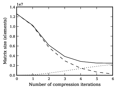
The considerations above motivates stopping compression early, after a significant reduction in the floating-point operation count has been achieved, but before the size of the precomputed data becomes too large (see Figure 3). Butterfly compression has the convenient feature that the blocks in the residual matrix consists of contiguous slices from columns of . By orienting so that rows are indexed by and columns by , the elements of the residual blocks can be computed on the fly from three-term recurrence formulas for the associated Legendre functions. We return to this topic in Section A.2.
As an example, consider and . The uncompressed matrix takes 64 MB in double precision. This can be compressed to 20% of the original size by using five levels of compression, with the uncompressed residual accounting for about 13% of the compressed data. If one instead stops after three levels of compression, then although the size of the compressed data has now grown to 24% of the original, 57% of this is made out of elements in . Since one only needs to store two elements for every column of 512 elements in and can generate the rest on the fly, stopping compression after three levels reduces the memory bus traffic and size of precomputed data by about 40%, at the cost of some extra CPU instructions. Note that the brute-force codes may simply be seen as the limit of zero levels of compression.
IV. Implementation & results
IV.1. Technology
The Wavemoth library is organized in a core part and an auxiliary part. The core is primarily written in C and contains the routines for performing spherical harmonic transforms. The auxiliary shell around the core is written as a Python package, and is responsible generating the precomputed data using the butterfly compression algorithm, as well as the regression and unit tests.
By writing the core in pure C we remain close to the hardware, and make sure the library can be used without Python. C remains the easiest language to call from other languages such as Fortran, C++, Java, Python, MATLAB, and so on. By using Python in the auxiliary support code we accelerate development of the parts that are not performance critical, and make writing tests a pleasant experience. Being able to quickly write up unit tests is an indispensable tool, as it allows optimizing the C code iteratively without introducing bugs. Since individual pieces of the C core is tested, there is both a public API for end-users and a private API that is used from Python to test individual C routines in isolation. Much of the support code is implemented in Cython [1], which bridges the worlds of Python and C.
The C core depends on files containing precomputed data, a Fourier transform library and a BLAS library. For the latter two we use FFTW3 [6] and ATLAS [26], respectively. Parts of the Wavemoth core is written using templates in order to generate many slight variations of the same C routine. We use Tempita22 2 http://pythonpaste.org/tempita/, a purely text-oriented templating language, and find this to be much more convenient for optimizing a computational core than the type-oriented templates of C++. During the precomputations, we use the open source Fortran 77 library ID33 3 http://cims.nyu.edu/˜tygert/software.html to compute the Interpolative Decomposition, and libpsht to generate the associated Legendre functions.
Unlike libpsht, we have not focused on portability, and Wavemoth is only tested on 64-bit Linux with the GCC compiler on Intel-platform CPUs. Computational cores are written using SSE intrinsics and 128-bit registers. More work is needed for optimal performance on the latest Intel micro-architecture, which support 256-bit registers, or on non-Intel platforms. Beyond that, we expect no hurdles in improving portability.
IV.2. Benchmarks


| No comp. | Intel () | AMD () | Precomputation time | |||
|---|---|---|---|---|---|---|
| Tol. | Tol. | Tol. | Tol. | (CPU minutes) | ||
| 32 | 130 KiB | – | – | – | – | 0.02 |
| 64 | 496 KiB | – | – | – | – | 0.03 |
| 128 | 2.0 MiB | 2.0 MiB | 2.0 MiB | 1.9 MiB | 1.9 MiB | 0.22 |
| 256 | 8.0 MiB | 8.0 MiB | 8.0 MiB | 7.1 MiB | 7.1 MiB | 2.6 |
| 512 | 27 MiB | 174 MiB | 187 MiB | 27 MiB | 27 MiB | 7.4 |
| 1024 | 102 MiB | 937 MiB | 988 MiB | 102 MiB | 170 MiB | 12 |
| 2048 | 389 MiB | 6.0 GiB | 5.8 GiB | 4.4 GiB | 4.3 GiB | 90 |
| 4096 | 1.5 GiB | 38 GiB | 35 GiB | 28 GiB | 27 GiB | 536 |
| 8192 | 5.8 GiB | 212 GiB | 208 GiB | – | – | 4380 |
Note. — The precomputation time quoted is the wall time taken to compute at tolerance on the Intel system, multiplied by the number of CPU cores used. We use 1 core for , and then scale up gradually to 64 cores at . The precomputed data is saved to a network file system.
| No compression | Tolerance | Tolerance | |
|---|---|---|---|
| 8 | 8.6e-16 | – | – |
| 16 | 1.4e-15 | – | – |
| 32 | 2.7e-15 | – | – |
| 64 | 5.8e-15 | – | – |
| 128 | 1.2e-14 | – | – |
| 512 | 5.1e-14 | 4.7e-14 | 1.9e-09 |
| 1024 | 1.3e-13 | 8.9e-14 | 2.4e-09 |
| 2048 | 2.7e-13 | 1.7e-13 | 3.1e-09 |
| 4096 | 6.4e-13 | 3.3e-13 | 3.7e-09 |
| 8192 | 2.2e-12 | 6.6e-13 | 4.2e-09 |
Note. — In each case, the transform of a single Gaussian sample is compared against libpsht double precision results.
We include benchmarks for two different systems with different memory bandwidth, as Wavemoth’s performance is deeply influenced by this aspect of the hardware. Figure 4 presents benchmarks taken on a 64-core 2.27 GHz Intel Xeon X7560 (Nehalem micro-architecture), which has a compute-to-bandwidth ratio of about 45:1. Figure 5 presents benchmarks taken on a 48-core 2.2 GHz AMD Opteron 6174. The compute-to-bandwidth ratio is in this case about 64:1, significantly worse than the Intel system44 4 The Intel system supports transfer of 13 billion numbers per second and has theoretical peak compute power 580 GFLOPS, using all 64 cores. The AMD system supports transfer of 6.5 billion numbers per second and has theoretical peak compute power of 422 GFLOPS, using all 48 cores. All numbers refer to double precision floating point.. The consequence is that butterfly compression gives less of an advantage, with only about four times speedup over libpsht at , compared to the corresponding six times speedup achieved on the Intel system. In the case of ten simultaneous transforms, libpsht achieves a very consistent 2x speedup which Wavemoth is not able to fully match, as most of our tuning effort has been on the single transform path.
The highest tested accuracy of for the Legendre transforms was chosen because current codes using the HEALPix grid only agree to this accuracy on high resolutions [20].
An important aspect of the systems for our purposes is the non-uniform memory access (NUMA). On each system, the CPU cores are grouped into eight nodes, and the RAM chips evenly divided between the nodes. Each CPU only have direct access to RAM chips on the local node, and must go through a CPU interconnect bus to access other RAM chips. For consistent performance we need to ensure that Wavemoth distributes the precomputed data in such a way that each CPU finds the data it needs in its local RAM chips. In the benchmarks we always use a whole number of nodes, so that computation power and memory bandwidth scale together. The exception is benchmarks using a single core, but in those cases, Wavemoth’s precomputed data fits in cache anyway.
Table 1 list the sizes of the precomputed data. To balance bandwidth and CPU requirements as described in Section III.4, the precomputation code takes a parameter , specifying the cost of floating point operations in the bandwidth-intensive butterfly matrix application stage relative to the cost of floating point operations in the CPU-intensive brute-force Legendre transform stage. The parameter was then tuned for the single-transform case for , resulting in optimal choices of on the Intel system and on the AMD system. Performing the precomputations scales as . In the case of no compression, we still store the precomputed quantities necessary for the Legendre recurrence relations in memory, as described in the appendix. Loading this data from memory is not necessarily faster than computing it on the fly, but doing so saved some development time.
All methods involved are numerically stable and well understood, so we do not include a rigorous analysis of numerical accuracy. Table 2 lists the relative error from transforming a single set of standard Gaussian coefficients per configuration. We use the relative error
| (24) |
where denote the result of libpsht and the result of our code. The discrepancies in the no-compression, high- cases are due to using a different recurrence for the associated Legendre functions, as described in Appendix A.2. As we did not compare with higher precision results, it is not clear whether it is our code, libpsht, or both, that loose precision with higher resolution. Note that the input data to the butterfly compression is generated using libpsht.
IV.3. Higher resolutions
Due to memory constraints we have not gone to higher resolutions than . Instead, we provide estimates for the number of required floating point operations. [25] provide similar estimates, but focus on the behavior for the Legendre transform for single rather than the full SHT.
At each resolution, we compress for 20 different , and fit the cost estimate
| (25) |
by least squares minimization in the parameters and . The final cost is then estimated by
| (26) |
since and has almost identical behavior. The results can be seen in Figure 2. For , the butterfly algorithm requires only 1% of the arithmetic operations of a brute force transform. The size of the precomputed data at this resolution is around 45 TiB in double precision, although this can be reduced by using the hybrid approach of Section III.4.
At low resolutions, the algorithm is bound by the operations of the brute-force Legendre transform. At high resolutions, the trajectory is clearly a better fit than the scaling conjectured by [25]. Note that the numerical evidence presented in [25] show that the average increases monotonically with , so it may indeed be the case that the rank property is not fully satisfied, or only satisfied conditional on . The benchmark results of [25] seem to be in agreement with the hypothesis as well.

IV.4. Comparison with other fast SHT algorithms
A widely known scheme for fast SHTs is the transform of [9], implemented in SpharmonicKit. It algebraically expresses a Legendre transform of degree as a function of two Legendre transforms of degree , resulting in a divide-and-conquer scheme similar to the FFT algorithms. Unfortunately, the scheme is inherently numerically unstable, and special stabilization steps must be incorporated. Also, it is restricted to equiangular grids, so that it can not be used directly with the HEALPix or GLESP grids. [27] benchmarks SpharmonicKit against the original HEALPix implementation (pre 2.20) and find that it is almost three times slower at . Keep in mind that libpsht, used in present releases of HEALPix, is about twice as fast as the original HEALPix implementation. Considering the above, we stop short of a direct comparison between Wavemoth and SpharmonicKit. Note that while SpharmonicKit achieves much higher accuracy of an SHT round-trip than HEALPix does, this is an effect of the different sampling grids being used, not of the computational method, and it is straightforward to extend the Wavemoth code to use the same grid as SpharmonicKit.
[17] uses a matrix compression technique similar to the one employed in this paper, which is independent of the pixel grid chosen. A matrix related to the of the present paper is locally approximated by truncated trigonometric series. The resulting SHT algorithm scales as . As shown in Figure 6, the code behaves very similarly to our code at medium resolution, as long as one do not require too much numerical accuracy. The size of the precomputed data is also of the same order, sometimes half and sometimes double that of Wavemoth’s data.
Note that libftsh appears to have potential for optimization for modern platforms, and this should be taken into account when comparing the algorithms. Due to its age, libftsh makes assumptions about 32-bit array sizes which prevents comparison at higher resolutions without porting libftsh to 64-bit. The libftsh code contains an implementation of the Legendre transforms only, and not of the full spherical harmonic transforms. It should be straightforward to modify Wavemoth to use libftsh for its Legendre transforms in order to perform full SHTs using this algorithm.
The compression scheme of [17] appears to be very competitive for low accuracy transforms, but less so if higher precision is needed. It may be fruitful to hybridize the algorithms of [25] and [17] and use both together to compress a single matrix. Even if that does not work, one can simply use whichever performs best for a given .
V. Discussion
There is significant potential in speeding up spherical harmonic transforms beyond the codes in popular use today. We achieved a 2x speedup at low and medium resolutions simply due to restructuring how the brute-force computations are done, and believe there is potential for even more speedup if time is spent on profiling and micro-optimization. In particular, our code is under-optimized for multiple simultaneous transforms.
At the highest resolutions in practical use in cosmology today, , use of the butterfly compression is borderline. One the one hand, it does yield an additional 2x speedup; potentially much more if one needs less accuracy. On the other hand, it requires between 30 and 40 GiB of precomputed data in memory, and the transportation of that data over the memory bus for every set of transforms. The result is a delicate balance between bandwidth and achieved speedup; for every number stored in the precomputed data, one might save 40 arithmetic operations, but then again computation is much cheaper than accessing system memory on present-day computer architectures.
In Section III.3, we note the existence of interpolation schemes that cut the necessary sample points for brute-force codes by two thirds in the case of the HEALPix grid; although performing the interpolation step does not come for free. It seems that the speedup from such interpolation alone could on the same order as what the butterfly algorithm achieves for the current needs of CMB research. The advantage is that it does not require nearly as much precomputed data, and is so much less architecture-dependent and easier to micro-optimize. In going forward we therefore anticipate spending more effort on direct interpolation schemes and less effort on matrix compression. For resolutions higher than those needed in CMB analysis, matrix compression schemes seem like the most mature option at the moment.
We have not discussed spin-weighted spherical harmonic transforms, which are crucial to analyzing the polarization properties of the CMB. However, [12] and [28] describe how the transform of a polarized CMB map can be reduced to three scalar transforms. This would additionally help amortize the memory bus transfer of the precomputed data. Alternatively, it may be possible to compress the spin-weighted spherical harmonic operators.
We consider Wavemoth an experimental code for the time being, and spherical harmonic analysis has been left out. This was done purely to save implementation time, and we know of no obstacles to implementing this using the same methods. The code also lacks support for MPI parallelization, although we expect adding such support to be straightforward. The only inter-node communication requirement is a global transpose of between the Legendre transforms and the Fourier transforms.
Appendix A Implementation details
A.1. Applying the compressed matrix representation to a vector
On modern computers, the primary bottleneck is often to move data around. Fundamental design decisions were made with this in mind. Looking at the compressed representations of in Section III.2, the immediate algorithm that comes to mind for computing or is the breadth-first approach: First compute , then permute the result, then compute , and so on. However, this leads to storing several temporary results for longer than they need to, since the rightmost permutations are very local permutations, and only the leftmost permutation is fully global. Therefore we traverse the data dependency tree set up by the permutations in a depth-first manner. The advantage of this approach is that it is cache oblivious when transforming a few vectors at the time. That is, it automatically minimizes data movement for any cache hierarchy, whereas breadth-first traversal will always drop to the memory layer that is big enough to hold the entire set of input vectors. Note that for transforming many maps at the same time, cache-size dependent blocking should be implemented in addition, but we have stopped short of this. Like [25], we also do the compression during precomputation depth-first, which ensures that, per , memory requirements go as even though computation time go as .
The core computation during tree traversal is to apply the interpolative matrices, e.g., or . Keep in mind that the -by- matrix contains the -by- identity matrix in a subset of its columns; making use of this is important as it roughly halves the storage size and FLOP count. Given an ID , we can freely permute the rows of , simply by permuting the columns of correspondingly. We do this during precomputation to avoid the unordered memory usage pattern of arbitrary permutations. Instead, we can simply filter the input or output vectors into the part that hits the identity sub-matrix and the part that hits the dense sub-matrix.
A.2. Efficient code for Legendre transforms
As mentioned in Section III.4, it is necessary to balance the amount of precomputed data to the memory bandwidth, so code is required to apply the residual blocks in to vectors without actually storing in memory. This means computing a cropped version of the Legendre transform,
| (A1) |
where for the even transforms and for the odd transforms. To compute we use a relation that jumps two steps in for each iteration [25]:
| (A2) |
with
and
This recurrence relation requires five arithmetic operations per iteration, as opposed to a more widely used relation which takes one step in and only needs four arithmetic operations per step [19, see, e.g.,]. However, since and may have different columns in the residual blocks of their compressed representations, relation (A2) is a better choice in our case.
For each block in we precompute , and , as well and for each for initial conditions. Note that in parts of its domain take values so close to zero that they can not be represented in IEEE double precision. However, in these cases is always increasing in the direction of increasing , so we can simply increase correspondingly. In fact, we follow libpsht and assume that the dynamic range of the input data is small enough, within each , that values of smaller than in magnitude can safely be neglected. As far as possible we group together six and six columns with the same and , for reasons that will soon become clear.
For an efficient implementation, the first important point is to make sure the number of loads from cache into CPU registers is balanced with the number of floating-point operations. The second is to make sure there are enough independent floating-point operations in flight simultaneously, so that operations can be pipelined. Thus,
- •
for performing a single transform with one real and one imaginary vector, the values of should never need to leave the CPU registers. Rather, we fuse equation (A1) and equation (A2) in the core loop. For multiple simultaneous transforms we save to cache, but make sure to process in small batches that easily fit in L1 cache.
- •
we process for several simultaneously. This amortizes the register loads of , and . It also ensures that there are multiple independent chains of computation going on so that pipelining works well.
In the single transform case with one real and one imaginary vector, we do the full summation for six at the time (when possible). The allocation of the 16 available 128-bit registers, each holding two double-precision numbers, then becomes three registers for , three for , three for the auxiliary data , and , six accumulation registers for , and one work register. The values are, perhaps counter-intuitively, read again from cache in each iteration, which conserves three registers and thus enables processing six in each chunk instead of only four without register spills. Finally, when the time comes for multiplying with , the auxiliary data is no longer needed, leaving room for loading .
On the Intel Xeon system, the routine performs at 6.46 GFLOP/s per core (71% of the theoretical maximum) when benchmarked on all the Legendre transforms necessary for a full SHT across 32 cores. The effect of instruction pipelining is evident; reducing the number of columns processed in each iteration from six to four reduces performance to 5.69 GFLOP/s (63%), and when only processing two columns at the time, performance is only 4.28 GFLOP/s (47%).
We skip the details for the multiple transform case, but in short, in involves the same sort of blocking performed for matrix multiplication, including repacking the input data in blocks. [7] provide an excellent introduction to blocking techniques. In this case the performance is 5.60 GFLOP/s (62%) per core when performing the Legendre transforms necessary for ten simultaneous SHTs.
The considerations above guided the choice of loop structure, which was then implemented in pure C using SSE intrinsics. We did not spend much time on optimization, so there should be room for further improvements, in particular for the multiple-transform path.
A.3. Data layout
The butterfly compression algorithm naturally leads to the following code organization for spherical harmonic synthesis:
- 1.
Since each is processed independently, we request input in -major ordering. Also, for multiple simultaneous transforms, the coefficients of each map are interleaved, which is optimal both for the butterfly algorithm and the brute-force cropped Legendre transforms. In most places, the real and complex parts of the input can be treated as two independent vectors, since is a real matrix.
- 2.
Compute all into a 2D array. Since each is processed independently, this ends up in -major ordering, like the input.
- 3.
While transposing the array into ring-major ordering, phase-shift and wrap around the coefficients, and perform FFTs on each ring. Rings must be processed in small batches in order to avoid loading cache lines multiple times.
A temporary work buffer with size of the same order as the input and output is used for . An in-place code should be feasible with the use of an in-place transpose.
A drawback compared to brute-force codes is that needs to first be written to and then read from main memory. Here, libpsht is instead able to employ blocking, so that a few rings at the time are completely processed before moving on. Our benchmarks do however indicate that this is not a big problem in practice. Also, for cluster parallelization using MPI, it would be natural to follow S2HAT [10, 23] in distributing the input data by and the output data by rings, which also leads to a global transpose operation.
Wavemoth stores the output maps in interleaved order, since FFTW3 is able to deal well with such transforms. The libpsht code is able to support any output ordering, although stacked, non-interleaved maps are slightly faster, so that is the ordering we use for libpsht in the benchmarks.
References
- [1] Behnel, S., Bradshaw, R., Citro, C., Dalcin, L., Seljebotn, D. S., & Smith, K. 2011 Computing in Science & Engineering, 13, 2
- [2] Cheng, H., Gimbutas, Z., Martinsson, P. G., & Rokhlin, V. 2005 SIAM J. Sci. Comput., 26, 4
- [3] Doroshkevich, A. G., Naselsky, P. D., Verkhodanov, O. V., et al. 2005, Int. J. Mod. Phys. D, 14, 275
- [4] Dutt, A., Gu, M., & Rokhlin, V. 1996 SIAM J. Numer. Anal., 33, 5
- [5] Eriksen, H. K., Jewell, J. B., Dickinson, C., Banday, A. J., Górski, K. M., & Lawrence, C. R. 2008 ApJ, 676, 1
- [6] Frigo, M., & Johnson, S. G. 2005 Proceedings of the IEEE, 93, 2
- [7] Goto, K., & van de Geijn, R. 2008 ACM Trans. Math. Softw., 34, 3
- [8] Górski, K. M., Hivon, E., Banday, A. J., Wandelt, B. D., Hansen, F. K., Reinecke, M., & Bartelmann, M. 2005 ApJ, 622, 2
- [9] Healy, D. M., Rockmore, D. N., Kostelec, P. J., & Moore, S. 2003 Journal of Fourier Analysis and Applications, 9, 4
- [10] Hupca, I.O., Falcou J., Grigori L., & Stompor R. 2010, INRIA Technical Report, No. RR-7409, arXiv:1010.1260
- [11] Jakob-Chien, R., & Alpert, B. K. 1997 Journal of Computational Physics, 136, 2
- [12] Kostelec, P. J., Maslen, D. K., Jr., D. M. H., & Rockmore, D. N. 2000 Journal of Computational Physics, 162, 2
- [13] Kunis, S., & Potts, D. 2003 Journal of Computational and Applied Mathematics, 161, 1
- [14] Martinsson, P. G., & Rokhlin, V. 2007 SIAM J. Sci. Comput., 29, 3
- [15] McEwen, J. D., & Wiaux, Y. 2011 Signal Processing, IEEE Transactions on, 59, 12
- [16] Michielssen, E., & Boag, A. 1996 IEEE Trans. Antennas Propag., 44, 8
- [17] Mohlenkamp, M. J. 1999 Journal of Fourier Analysis and Applications, 5, 2
- [18] O’Neil, M., Woolfe, F., & Rokhlin, V. 2010 Applied and Computational Harmonic Analysis, 28, 2
- [19] Press, W., H., Teukolsky, S., A., Vetterling, W., T., & Flannery, B., P. 2007 Numerical Recipes (3rd ed.; New York, Cambridge University Press)
- [20] Reinecke, M. 2011 A&A, 526, A108
- [21] Rokhlin, V., & Tygert, M. 2006 SIAM J. Sci. Comput., 27, 6
- [22] Suda, R., & Takami, M. 2002, Mathematics of Computation, 71, 238
- [23] Szydlarski M., Esterie P., Falcou J., Grigori, L., Stompor, R. (2011), INRIA technical report, No. RR-7635, arXiv:1106.0159
- [24] Tygert, M. 2008 Journal of Computational Physics, 227, 8
- [25] Tygert, M. 2010 Journal of Computational Physics, 229, 18
- [26] Whaley, R. C., Petitet, A., & Dongarra, J. 2001 Parallel Computing, 27, 1-2
- [27] Wiaux, Y., Jacques, L., Vielva, P., & Vandergheynst, P. 2006 ApJ, 652, 1
- [28] Wiaux, Y., Jacques, L., & Vandergheynst, P. 2007 Journal of Computational Physics, 226, 2
- [29] Yarvin, N., & Rokhlin, V. 1999 SIAM J. Numer. Anal., 36, 2